Sage Journals: Discover world-class research

Abstract

In the automotive field, the customer requirements for low interior noise and pleasant sound quality inside a vehicle are getting higher and higher. Various national and international regulatory authorities established and reviewed vehicle interior noise for the past years. Besides, lots of studies have shown that vehicle noise can influence the driver’s perceptions and also his or her driving capabilities. To succeed in this scenario, all manufacturers are investing in technology and research in order to improve their component performance. Working on the noise source so as to reduce the seriousness of these noise problems can be really effective. However, various engineering techniques are available to deal with noise and sound-measuring instruments, and systems can help to identify the nature of the problem and they can also be helpful in determining the right procedure to analyse the noise problem. This work proposes a procedure to evaluate the noise originated from an electronic steering column lock device which is used to lock and unlock the steering wheel according to European safety requirements. In particular, different standards and requirements for loudness evaluation have been discussed and the formulation of a straightforward procedure, which can be used to evaluate the loudness according to costumer’s requirements, is defined.

Keywords

Electronic steering column lock sound analysis loudness sound measurement

Introduction

In recent years, all kinds of vehicle manufacturers, for example, military, aircraft and mainly automobile industries, have noise reduction and control as one of the mail goals due to the increasing requirements for low noise emission. In an effort to decrease and control the interior noise and levels of vibration of not only the above-mentioned vehicles but also other equipment, devices and machines, many techniques have been developed:¹ noise source identification (NSI) techniques^2–10 and active and passive control methods.^11–15 In particular, passive controls can benefit of the use of innovative materials, such as piezoelectrics, shape memory alloys,¹¹ magnetostrictive materials¹² and chiral unit cells,^13–18 and their mechanical properties can be designed within very large range of modulus and Poisson’s ratio values. Active controls require external power sources and complex controllers.^19–23

The main usage of NSI techniques is to identify the noise emission from any kind of device including vehicles and machines. This purpose can be reached by identifying the main parameters that characterize a noise sub-source of an object such as position, frequency and sound power radiation. In this way, it is possible to recognize the most important contributions to the total noise and then make efficient redesign decisions or simply applying insulation techniques. The most common techniques available and used nowadays are based on three methods: sound mapping, near-field acoustic holography (NAH) and beamforming. Sound mapping method gives rise to three different NSI techniques, namely, sound pressure level (SPL), sound intensity and selective intensity, characterized by increasing cost and level of detail. The techniques based on NAH are mainly spatial transformation of sound fields (STSF), non-stationary STSF and statistically optimized near-field acoustical holography (SONAH). The last technique for NSI identification is beamforming; it allows directional NSI for exterior vehicle noise at medium-to-high frequencies. Basically, this technique enables the estimation of sound pressure contributions at the array grid from different directions.

Christensen and Hald⁷ worked on a sound field captured by an array of microphones. They used a standard delay-and-sum beamformer whose resolution is limited to around one wavelength, Gade and Hald⁸ highlighted that a refined beamforming technique based on different algorithms, for instance, non-negative least squares (NNLS) and deconvolution approach for mapping acoustic sources (DAMAS), might be applied to increase the spatial resolution. A particular technique is the moving source beamforming, a useful technique for noise sources which are in motion, for instance, a car pass-by, an aircraft fly-over and others.⁹ Spherical beamforming is essentially an extension of a planar beamforming. This type of configuration has the advantage of being able to cover all directions with direction-independent angular resolution. It is mainly used in enclosures, for instance, cabins and rooms although it can also be used in a free field.

According to Peterson,²³ loudness is the sensation value of the human perception of sound volume. The evaluation of this parameter provides the human sensation of sound volume of acoustic signals on a linear scale. In ISO 226,²⁴‘equal loudness contours’, obtained from a wide reference basis published from 1983 to 2002, are plotted. These contours can be used in many applications such as noise measurement in car interiors, engines, exhaust ducts and domestic appliances. In case of more complex sound situations, other parameters and functions can help. The critical bandwidth is a quantitative parameter describing the ear frequency resolution. The ISO 532²⁵ in the so-called ‘method B’ describes a graphical method for the loudness calculation in case of complex stationary sounds from third octave bands, whereas the German specification DIN 45631²⁶ provides a comparable but computational method for the same calculation.

In acoustics, loudness is usually expressed in dB(A),²⁷ and the perceived loudness is better described when critical bandwidths are used. Assuming that ‘a relative change in loudness is proportional to a relative change in intensity’,²⁸ a parameter describing a specific loudness is defined basing on the third-octave band levels following a power law. Specific loudness (N′) is expressed in sone per Bark. The loudness value (N) is calculated as the integral of this curve and is expressed in sones.

The most recent version of the ISO 532 standard for calculating loudness level is from 1975. As mentioned before, it describes a method, the so-called Zwicker process, for manually plotting data on special graphs to determine a loudness value. Current commercially available sound quality systems reference this standard, but use a computer algorithm²⁹ that is not documented in the standard. Some systems also use more advanced (and, as of yet, not standardized) processes also documented by H Fastl and E Zwicker.³⁰ However, it is known that the results of analysing the same recorded data with different systems using the more advanced versions of Zwicker method may not always agree due to the lack of standardization.

The procedure as reported by ISO 532 starts from time signal elaboration and third-octave level calculus. Then, the procedure for the graphic calculation of loudness level consists of three steps based on a set of graphs. In a general way, the critical bands of frequencies under 250 Hz are grouped, since in the lower frequency range the critical bands are broader than a third band. The critical bands of higher frequencies can be approximated by means of third-octave bands in order to use the third-octave level for further processing. These levels are then entered into a diagram and the area enclosed by the whole stepped figure corresponds to the total loudness.

The partial loudnesses of the noise are entered as thick continuous lines. The area under the curve is equivalent to the one under the dotted horizontal line. The total loudness can be taken through the height of this line from the scales on the left and right.

On the other hand, DIN 45631 indicates a BASIC programme,²⁹ which approximates the said graphic procedure. This calculation method is identical to the method via filtering described above. As far as it can be foreseen, this standard will evaluate the loudness in the same way as the ISO, but will also save a valuable time and handwork.

To summarize, ISO 532 describes two similar methods useful for calculation of the stationary sound loudness, one based on the studies by SS Stevens and the other on studies by E Zwicker. Also, the DIN 45631 provides the same evaluation, but it uses a computer algorithm to speed up the process.

Moreover, the DIN 45631/A1³¹ describes a method to handle with time-varying and impulsive sounds. Other techniques are proposed by Zwicker and Fastl²⁸ and Moore et al.³² In particular, for the study of impulsive sounds, Boullet³³ developed a specific technique (LMIS, loudness model for impulsive sounds).

The above described techniques may be used in order to achieve a suitable analysis and control of noise for automotive vehicles and sub-assemblies under different vehicle operating conditions, but in order to choose a method and subsequently a technique, it is necessary to consider several other parameters such as cost, space, equipment, time and others.

This work reports an analysis led on an electronic steering column lock (ESCL) device.

Certainly, the operation of an ESCL device is not the main source of noise inside any vehicle cabin. However, it is known that the whole assembling gives rise to an audible noise during the locking and unlocking processes. Moreover, vehicle manufacturers and regulatory authorities are getting more and more demanding for noise reduction not only for comfort but also, and more important, for safety reasons.

In this article, different standards and requirements for loudness evaluation have been discussed and the formulation of a straightforward procedure, which can be used to evaluate the loudness according to costumer’s requirements, is defined.

The whole process can be subdivided into two major steps. First, the noise is measured and sampled (data acquisition). Second, MATLAB® subroutines are used to process the acquired data and to evaluate parameters that better represent the human perception of sound, for instance, loudness. The results yield a better parameter of the human being hearing capabilities as stated by Zwicker et al.²⁹ and Fastl and Zwicker³⁰

General frame

According to the ISO 3745,³⁴ sound pressure p (Pa) refers to the difference between instantaneous and static pressure.

The changes in sound pressure can be huge and then it becomes convenient to express sound pressure (dB) and then it is defined as SPL or L_p with respect to a reference sound pressure. For airborne sounds, the reference pressure is generally 20 µPa.

The equation used to evaluate SPL is

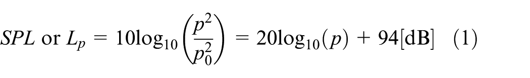
SPL or L_{p} = 10 \log_{10} (\frac{p^{2}}{p_{0}^{2}}) = 20 \log_{10} (p) + 94 [dB]

(1)

where p is the root-mean square sound pressure and p₀ is the international reference pressure (20 µPa).

Sound power (W) is the average rate a source radiates sound energy. Sound power level (PWL or L_W) is defined as the sound emission, which is continuously radiated from the sound source regardless of the distance.³⁴ A reference sound power was established to 10⁻¹² W. No direct measurement for the power level of a source is available. However, power level of a machine can be computed from sound pressure measurements. ISO and other standards show procedures to evaluate such coefficient.

The sound power level is

PWL or L_{w} = 10 \log_{10} (\frac{W}{W_{0}}) = 10 \log_{10} (W) + 120 [dB]

(2)

where W is the acoustic energy of the source given in Watts (W) and W₀ is the international reference sound power of 10⁻¹² W.

According to István and Beranek,³⁵ with spherical source, the radiated sound wave is spherical and the total power emitted in all directions is W. Sound intensity is defined as the continuous flow of power carried by a sound wave through an incrementally small area at a point in the space; it decreases with distance in proportion with sound.

The frequency spectrum of a time domain signal can be calculated, via a Fourier transform of the signal; the resulting values are usually presented as amplitude and phase versus frequency.

Narrow band, octave analysis and fractional octave analysis³⁶ provide sound description in different frequency bands.

In the study by Peterson,²³ an octave band is defined as a frequency band where the highest frequency is twice the lowest frequency. Octave bands or 1/3 octave bands are most often used when measuring sound.

In order to identify energy spikes, a more detailed noise analysis (e.g. using one-third octave band) can be performed. To increase accuracy, a narrow band analysis over specified narrow frequency ranges could be carried out.

Fastl and Zwicker³⁰ suggest that the fast Fourier transform (FFT) spectrum is probably not of interest when approaching the psychoacoustic measures, whereas loudness, harshness or annoyance subjective qualities are trying to estimate a perception.

Octave representation can also be obtained from the FFT of the time domain signal, with some differences in resolution at low frequencies.

The unit of loudness are sone and phons. As a reference, the loudness of a 1000 Hz tone with an SPL of 40 dB produces a loudness level of 1 sone (40 phons).

The human ear is less sensitive to sound pressure variations in the low frequencies than in the higher frequencies.

Case study

In this article, the sound analysis of the actuation of an automotive electronic steer column locking (ESCL) is analysed.

Regulations such as ECE R18 UN, EEC 74/61 and 95/56 Europe, FMVSS 114 US, FMVR 541/542/543 US and Article 12-2 Japan yield a set of rules and requirements for reliable performance and quality operation of this device.

The worm-shaft transmits the high-speed rotation of DC motor to low-speed rotation of the wheel. Subsequently, the screw joint, which is placed in the inner part of the gear, transmits the wheel (gear) rotation into linear vertical movement of the lock bolt.

The whole assembling gives rise to an audible noise during the locking and unlocking processes and noise reduction is required for comfort and safety reasons.

Materials and methods

Five different types of ESL have been tested from three different competitors; their noise emission was measured. The ESCL may be placed at four positions in a vehicle cabin but only two were considered. In the first one, the pin lock was pointing upwards (configuration G) and in the second one facing downwards (configuration F). Five measurements of each microphone were acquired for each of the operating procedures (locking and unlocking) and for each configuration (G and F); 300 measurements were performed. Subsequently, the signals containing the pressure variation in function of time were sampled and processed.

A hemi-anechoic room (5 m × 5 m × 3.5 m, Figure 1) at SCS-Euroacoustics (Avigliana, Torino, Italy) was used for the noise measurement. Since there is no international standard providing information about the measurement configuration, the acquisitions were specifically based on the requirements of internal standards of automotive companies.

Figure 1.

Hemi-anechoic chamber.

The measurements were performed at the distances of 100 mm (A), 500 mm (B) and 1000 mm (C) distance and perpendicular to the centre of the lock pin face (Figure 2). The frequency range of interest was the whole audible spectrum (from 20 Hz to 20 kHz). A sample frequency f_s of 51.2 kHz was used.

Figure 2.

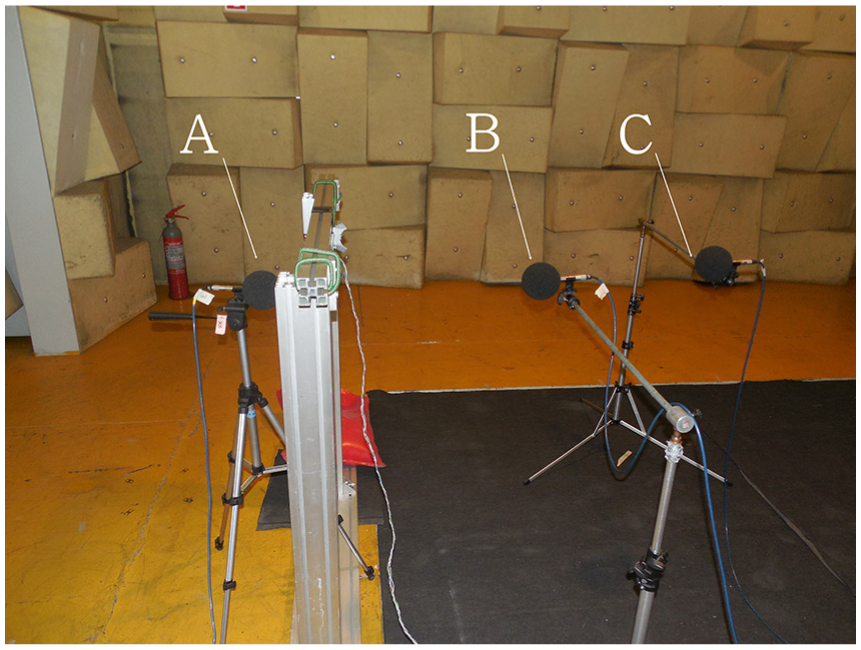
Microphone positioning.

To avoid structure-borne noise, the devices have been elastically hanged up and isolated from any object that may propagate the vibration during operation (Figure 3).

Figure 3.

Elastic fixing of the ESCL.

The background noise was measured by the three microphones to verify the fulfilment of measurement requirements.

The signal analysis process can be subdivided into two major steps. First, the noise is measured and sampled (data acquisition). Then, MATLAB® subroutines are applied to process the acquired data by means of 1/3 octave analysis and to evaluate parameters that better represent the human perception of sound, for instance, loudness. The results yield a parameter of the human being hearing capabilities as stated by Alton Everest²⁷ and Zwicker and Fastl.²⁸

The frequency analysis of the signal was carried out by means of Constant Percentage Bandwidth (CPB) analysis, 1/3 Octave bands.

A dedicated MATLAB® code was implemented to perform the signal conditioning and psychoacoustic parameter evaluation of sampled signals in time.

Some of the used functions were based on an open-source code and can be found and downloaded in MathWorks website.

Both the ANSI S1.11³⁶ and IEC 61620³⁷ specify one-third octave filtering. The work of Proakis and Manolakis³⁸ points out many methods that are available for the design of a digital filter from given specifications. The ANSI standard specifies the design goal and indicates the design method that must be used (Butterworth filters and the bilinear transformation). The code in MATLAB® was written using the ANSI standard.

To solve instabilities and other design problems, a multirate filter bank was used.³⁸

In order to estimate loudness without using a psychoacoustic test, several models are proposed in technical literature. In Table 1, a summary of models and respective applications is reported.

Table 1.

Summary of the models.

Model function	Steady sound	Time-varying sound	Impulsive sound
ISO 532 B/DIN 45631 (Zwicker)	X
DIN 45631/A1		X
Zwicker for temporally variable sounds		X
Moore et al. for time-varying sounds		X
Boullet-loudness model for impulsive sounds			X

According to the companies’ requirements, the ESL loudness should be calculated according to DIN 45631. However, the validity of this method has been questioned for time-varying and impulsive sounds³⁹ because of dependence of subjective loudness on sound duration for short bursts of sound.

Results and discussion

Experimental setup validation

Therefore, this section will show some results of one ESCL.

In Figure 4, background noise acquisition and processing, obtained by microphone A and C respectively, are reported as an example.

Figure 4.

Background noise: microphone position A (left) and C (right).

In Table 2, the requirements and results are reported. The test room complies with the specifications and it is suitable for the measurements.

Table 2.

Background noise requirements.

Requirements	Value required	Microphone A	Microphone B	Microphone C
Specific loudness (from 0 to 5 bark)	⩽0.2 [sones/bark]	Yes	Yes	Yes
Specific loudness (higher than 5 bark)	⩽0.1 [sones/bark]	Yes	Yes	Yes
Total loudness	⩽1.2 (sone GF)	Yes (0.06 sone GF)	Yes (0.063 sone GF)	Yes (0.09 sone GF)

A total of 60 measurements were carried out per each specimen.

As an example, in Figure 5, the results of five repetitions of the measurements in configuration F (lock bolt moving downwards during locking) are depicted for one microphone position. The five measurements of each microphone are superimposed in one graph to better verify the similarity of the measurements.

Figure 5.

Signal analysis (1/3 octave): configuration F – microphone A. Different lines show the measurement repetitions (m1–m5).

It results that acquisitions have a good repeatability for both configurations, except for some samples with configuration F at low frequencies. However, as can be noticed comparing the third octave spectrum of the ESCL noise measurements with the third octave spectrum of background noise, this device generates mainly high-frequency signals. Therefore, those differences at low-frequency are due to the variation of the energy inside the chamber, coming from electronic devices. The measurements can then be considered suitable for the noise analysis, detailed in the following section.

Frequency analysis and loudness evaluation

For the loudness calculation, the third-octave spectrum analysis provides the specific loudness and the total loudness according to DIN 45631 Standard, even though it is not the most convenient analysis method to be employed for this type of signal, as reported by Blommer et al.³⁹ In Figures 6 and 7, the sound analysis of two test configurations are reported as an example. In the upper plot, the sampled signal (Pressure (Pa) vs time (s)) is reported; the middle plot reproduces the one-third octave frequency bands of this signal; the lower plot reports the specific loudness with respect to the critical bands (Bark) and the total loudness, estimated from the previous values of third-octave bands.

Figure 6.

Configuration G: microphone A, locking.

Figure 7.

Configuration F: microphone A, unlocking.

Comparing the loudness graphs (third plot) of each figure, it is possible to identify the most critical configuration. In general, it is clear that the configuration with pivot downwards (F) has a worse performance than the configuration with pivot upwards (G); furthermore, by analysing the results of the different operations of configuration A, it is evident that the unlocking operation is the movement that produces more noise.

Comparison with other loudness evaluation methods

In the literature, other procedures, other than ISO 532 and DIN 45631, are described to examine not steady sounds. The works by Zwicker, Moore and Boullet suggest other procedures to handle time-varying and impulsive sounds. Bloomer et al.³⁹ state that impulsive sounds are characterized for short bursts that last less than 200 ms. In the present case, as the noise lasts for over than 350 ms, it cannot be considered an impulsive noise. As a consequence, the most suitable analysis for this sound should employ temporally varying signal methods. In this work, Zwicker’s and Moore’s algorithm has been implemented based on an already existing MATLAB code written by Genesis⁴⁰ and will be used to analyse the measurement of samples in its critical configuration (lock bolt downwards during unlocking) for the microphone positioned at 500 mm away from the source.

The above-mentioned models of loudness for time-varying sounds are similar in their principle to steady sound models. They take into account temporal masking, and the loudness is determined as a function of time.

Figure 8 displays the main stages in loudness calculation for both models.

Figure 8.

Flow chart: procedure for the evaluation of the loudness of time-varying sounds.

Fastl and Zwicker proposed a loudness model for time-varying sounds.³⁰ This model considers the temporal masking effect for the loudness calculation. As a matter of fact, a signal can be masked or difficult to be detected if it is closely preceded by another signal (posterior masking) or by a signal that closely follows it (previous masking). Zwicker’s model, however, considers only the first effect.

In this model, depending on signal intensity and duration, the masking effect is considered to last for a ‘long’ time after the end of the signal. Temporal masking is modelled by a discharge of capacitors.

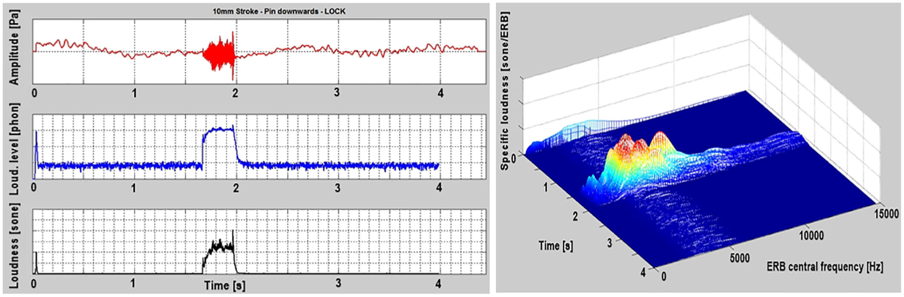
Figure 9 illustrates the results of the signal analysis using the Zwicker’s method described above. Note that Zwicker’s model allows the calculation of loudness as a function of time, but it does not give the overall loudness of time-varying sounds.

Figure 9.

Instantaneous loudness (left) and waterfall representation (right) according to Zwicker’s method – unlocking, configuration F.

Moore’s and Glasberg’s work⁴¹ has also developed a loudness model for time-varying sounds. For the loudness analysis, this method develops a procedure similar to previous methods, but with a finite impulse response (FIR) filter.

The filter shape depends on sound level. Actually, the filter slopes at low frequency become less steep when the level increases. The curve providing the output amplitude of each filter for a certain level models the excitation diagram. Moore’s method makes use of a multi-resolution spectral analysis by Fourier transform to evaluate this diagram. The analysis is performed on relatively long segments (64 ms) so as to obtain a resolution at low frequencies comparable to that of auditory system. In the case of high frequencies, shorter windows (2 ms) are used.

Six FFTs are then calculated in parallel, with temporal windows duration of 64, 32,16 8, 4 and 2 ms. These FFT calculations are used to measure the level in bands 20–80 Hz, 80–500 Hz, 500–1250 Hz, 1250–2540 Hz, 2540–4050 Hz and 4050–15,000 Hz, respectively. It is important to observe that some temporal overlap in the analysis is obtained if the excitation diagram is calculated from the spectrum with data extraction step equal to 1 ms.

To evaluate instantaneous loudness, it is assumed that it would correspond to the overall activity inside the auditory nerve on a period of time of about 1 ms. The instantaneous loudness calculation is obtained from the excitation diagram,⁴¹ which is then transformed into specific loudness. In a considered time interval, the area subtended to the loudness curve represents the instantaneous loudness.

Figure 10 shows the results of the signal analysis using Moore’s method for the measured noise of the sample in its critical operation. Turning to Moore,⁴¹ it can be found that equivalent rectangular bandwidth (ERB) bands are analogous to critical bands (i.e. a range of frequencies, which are grouped into one band because human hearing combines sound stimuli that are situated in close proximity of each other in frequency). Moreover, as expected, the models provide different numerical results. Yet, it is important to remind that these values are coming from two different models and thus are not directly comparable.

Figure 10.

Instantaneous loudness (left) and waterfall representation (right) according to Moore’s method – locking,configuration G.

Conclusion

Different standards and requirements for loudness evaluation have been discussed aiming at the definition of a procedure to evaluate noise loudness as an index of noise comfort in the vehicle cabin.

This research highlights that for the type of analysed noise (time-varying noise) the required standard procedure is not the most pertinent, as they are best employed for steady sounds. Besides that, no updating has been performed to the recommended standard for years. As a matter of fact, the companies’ requirements are based on the ISO Standard from 1975.

In this context, the scientific literature was reviewed and some new methods for loudness calculation (e.g. Zwicker’s and Moore’s method) were found; however, they have not been standardized and consequently they give rise to different results.

Finally, a review of techniques for noise control was described and future works may use them along with other tools in order to control and to improve the noise emission of mechanical systems.

Footnotes

Handling Editor: Guian Qian

Declaration of conflicting interests

The author(s) declared no potential conflicts of interest with respect to the research, authorship, and/or publication of this article.

Funding

The author(s) received no financial support for the research, authorship, and/or publication of this article.

ORCID iD

Raffaella Sesana

References

Ginn

Haddad

Noise source identification techniques: simple to advanced applications. In: Proceedings of acoustics, Nantes, 23–27 April 2012, pp.1781–1786. https://hal.archives-ouvertes.fr/hal-00810618

Hald

STFS – a unique technique for scan-based near field acoustic holography without restrictions on coherences, vol. 3. Copenhagen: Brüel & kjæer, 1989, pp.1–27.

Hald

Patch nearfield acoustical holography using a new statistically optimal method. Proc Internoise 2003; 2003: 2195–2202.

Hald

. Patch holography in cabin environments using two-layer handheld array with extended SONAH algorithm. In: 6th European Conference on Noise Control: Advanced Solutions for Noise Control, EURONOISE 2006, Tampere, Finland, 30 May–1 June 2006, pp. 2275. https://www.scopus.com/inward/record.uri?eid=2-s2.0-84872495718&partnerID=40&md5=515676c3cb0c0d5fe6d04d2d3bab9a14

Hald

Mørkholt

Panel contribution analysis in a vehicle cabin using a dual layer handheld array with integrated position measurement. SAE technical paper 2009-01-2171, 2009.

Hald

Mørkholt

Hardy

et al . Array based measurement of radiated and absorbed sound intensity components. J Acoust Soc Am 2008; 123: 2899–2904.

Christensen

Hald

Beamforming. Copenhagen: Brüel & kjæer, 2004, pp.1–48.

Gade

Hald

Noise source identification with increased spatial resolution used in automotive industry. J Acoust Soc Am 2012; 13: 9–13.

Ginn

Newton

Contribution analysis in pass-by testing using moving source beamforming. SAE technical paper 2011-01-1669, 2011.

10.

Haddad

Hald

3D localization of acoustic sources with a spherical array. J Acoust Soc AM 2008; 123: 2812–2816.

11.

Hassan

Scarpa

Ruzzene

et al . Smart shape memory alloy chiral honeycomb. Mater Sci Eng A 2008; 481–482: 654–657.

12.

Deng

Dapino

MJ.

Review of magnetostrictive materials for structural vibration control. Smart Mater Struct 2018; 27(11): 113001.

13.

Wen

et al . In plane mechanical properties of tetrachiral and antitetrachiral hybrid metastructures. J Appl Mech: T ASME 2017; 84: 081006.

14.

Tao

Xia

et al . Mechanical properties of hierarchical anti-tetrachiral metastructures. Extreme Mech Lett 2017; 6: 18–32.

15.

Song

Liang

et al . Mechanical properties of anti-tetrachiral auxetic stents. Compos Struct 2018; 185: 381–392.

16.

Xia

Song

Sun

et al . Mechanical properties of 3D isotropic anti-tetrachiral metastructure. Physica Status Solidi B 2017; 2017: 1700343.

17.

Geng

Niu

et al . Novel chiral structured force sensor inspired by towel gourd tendrils. Extreme Mech Lett 2018; 20: 104–111.

18.

Niu

et al . Deformation mechanism of 3D chiral metamaterials. Sci Rep 2018; 8: 12575.

19.

Frankovich

The four-fold method of noise and vibration control. Indianapolis, IN: E-A-R Specialty Composites, 2005.

20.

Liu

Lee

Passive and active interior noise control box structures using the structural intensity method. Appl Acoust 2006; 67: 112–134.

21.

Song

Saito

Haddad

Improved noise source identification using sound quality metrics mapping in vehicle noise measurements. SAE technical paper 2011-01-1671, 2011.

22.

Snyder

SD.

Active noise control primer. Modern acoustics and signal processing. New York: Springer, 2000.

23.

Peterson

APG

. Hand book of noise measurement. 9th ed. Concord, MA: GenRad, 1980.

24.

ISO 226:2003. Acoustics – normal equal-loudness-level contours.

25.

ISO 532: 1975. Acoustics – method for calculating loudness level (Method B).

26.

DIN 45631. Berechnung des Lautstärkepegels und der Lautheit aus dem Geräuschspektrum. Deutsches Institut Für Normung, 1991. In: Zwicker

Fastl

(eds) Psychoacoustics: facts and models. 3rd ed. Berlin: Springer, 2007.

27.

Alton Everest

Ken

Pohlman

. Master handbook of acoustics. 5th ed. New York: McGraw-Hill, 2009.

28.

Zwicker

Fastl

Psychoacoustics: facts and models. 3rd ed. Berlin: Springer, 2007.

29.

Zwicker

Fastl

Dallimar

Basic program for calculating the loudness of sounds from their 1/3-Oct band spectra according to ISO 532 B. Acustica 1984; 55: 63–67.

30.

Fastl

Zwicker

Psychoacoustics facts and models. 2nd ed. Berlin: Springer, 2006.

31.

DIN 45631/A1. Berechnung des Lautstärkepegels und der Lauheit aus dem Geräuschspektrum–Vefahren nach E.Zwicker (Calculation of loudness level and loudness from the sound spectrum – Zwicker method). Änderung 1: Berechnung Der Lautheit Zeitvarianter Geräusche, Deutsches Institut Für Normung, 2008.

32.

Moore

BCJ

Ashmore

Hagggard

New developments in hearing and balance: British medical bulletin. Oxford: Oxford University Press, 2002.

33.

Boullet

. The loudness of impulsive sounds: perception, measures and models. PhD Thesis, L’Universite de la Mediterrannee Aix-Marseille II, Marseille, 2005.

34.

ISO 3745:2012. Acoustics – determination of sound power levels and sound energy levels of noise sources using sound pressure-precision methods for anechoic rooms and hemi-anechoic rooms.

35.

István

Beranek

LL.

Noise and vibration control engineering – principles and applications. Hoboken, NJ: John Wiley & Sons, 2006.

36.

ANSI S1.11. Specification for octave-band and fractional-octave-band analog and digital filters.

37.

IEC 61260:1995. Electroacoustics: octave-band and fractional octave-band filters.

38.

Proakis

Manolakis

Digital signal processing: principles, algorithms and applications. 3rd ed. New York: Prentice Hall, 1996.

39.

Blommer

Otto

Wakefield

et al . Calculating the loudness of impulsive Sounds. SAE technical paper 951311, 1995.

40.

Genesis, 2009, www.genesis-acoustics.com

41.

Moore

BCJ

Glasberg

. A model for the prediction of thresholds, loudness and partial loudness. Audio Eng Soc 1997; 45: 224–240.

Loudness calculation procedure to study electronic steering column lock noise measurement

Abstract

Keywords

Introduction

General frame

Case study

Materials and methods

Results and discussion

Experimental setup validation

Frequency analysis and loudness evaluation

Comparison with other loudness evaluation methods

Conclusion

Footnotes

Declaration of conflicting interests

Funding

ORCID iD

References