Sage Journals: Discover world-class research

Abstract

Traffic flow parameters have been found to significantly affect crash risk at micro-levels. If such effects do exist at macro-levels, at least two benefits could be expected: (1) the performance and estimates of planning-based crash models could be improved and (2) useful safety knowledge could be provided for regional traffic management. In this article, a flow-based spatial unit was developed by a graph-cut minimization method, based on which regional management strategies are often applied. The graph-cut method partitioned the central area of Kunshan, China, into multiple sub-regions (i.e. graph-cut unit), considering traffic density homogeneity. Bayesian Poisson lognormal models with conditional autoregressive priors were utilized to examine the safety effects of traffic flow parameters, based on the traditional planning-based units and the flow-based graph-cut units. According to the results, no significant traffic flow effect was found for the traffic analysis zone–based model. Traffic flow parameters resulted in a decreased model performance and potential endogeneity issues for the census tract–based model. However, traffic flow effects were found significant for the graph-cut-based model, with an improved model performance. In general, the safety effects of macro-level traffic flow need to be considered for flow-based units developed for regional management.

Keywords

Macro-level crash modeling flow-based spatial unit graph-cut minimization method traffic homogeneity Bayesian modeling

Introduction

Macro-level crash models have been extensively developed to identify the safety effects of demographic, socioeconomic, and lane use factors, providing safety knowledge for decision-makers in the planning stage. In recent years, macro-level traffic flow characteristics have gained increased attention and a number of regional control strategies have been studied for regional management strategies, such as perimeter and boundary flow control,^1–3 regional route guidance,^4–6 and regional signal control.^7–9 Since it is well known that traffic flow parameters are associated with crash risk at micro-levels,¹⁰ the potential existence of traffic flow effects on crash risk at macro-levels may affect the safety performance of regional management strategies. Moreover, macro-level crash models with planning purposes may also be improved by considering such traffic flow effects (if significant), in terms of model performance and estimates. As for macro-level crash models, the modifiable areal unit problem (MAUP) is a critical issue that model performance and estimates (i.e. effects) could significantly vary by different spatial units.^11–19 Many spatial units have been examined in previous literature, including traffic analysis zones (TAZ), census tracts (CT), census wards (CW), block groups (BG), countries, and states.^16–18 Most of them are planning-based spatial units developed by administrative/political and long-term planning considerations (e.g. TAZ, CT, CW, and countries).^20,21 It is unknown that the safety effects of traffic flow parameters can be properly identified based on such units, since most were developed regardless of traffic flow parameters. However, for regional management purpose, flow-based units were suggested by aggregating areas with homogeneous traffic flow characteristics.²² In doing so, macro-level traffic flow was observed with similar characteristics with micro-level traffic flow, based on which regional management strategies can be easily applied. However, limited research has been identified to explore the effects of macro-level traffic flow parameters on crash risk for either planning-based or flow-based spatial units. For planning-based units, such effects, if exist, could affect model performance and estimates. For flow-based units, exploring such effects would help professionals better understand potential safety impact of regional management strategies.

Thus, in this article, we will examine the safety effects of macro-level traffic flow parameters based on three different spatial units. Two are planning-based units (i.e. TAZ and CT) and the other one is a flow-based unit. The flow-based unit was developed using a graph-cut (GC) minimization algorithm, considering traffic flow homogeneity. The objectives of this research are two-fold: (1) examine whether macro-level traffic flow parameters need to be considered for planning-based crash models and (2) provide some useful safety knowledge of macro-level traffic flow for the development of regional traffic management strategies.

Methodology

Flow-based spatial unit development

Ji and Geroliminis²³ introduced a GC minimization algorithm to partition an urban traffic network into multiple sub-regions, based on traffic density homogeneity. Based on such flow-based unit, macro-level traffic flow was found to have similar characteristics with micro-level traffic. In doing so, regional perimeter control approach can be applied to improve traffic condition for mixed urban network.^2,3 Thus, in this study, we will also utilize a GC method to develop a spatial unit for macro-level crash modeling, in order to add safety knowledge to regional traffic management.

GC minimization problem

A GC minimization method is introduced to partition a subject research area into multiple sub-regions, considering intersections as nodes and roadways as edges. Suppose the node set V in an undirected graph $G = (V, E)$ , where E denotes the set of edges in G. Assume that each edge between two vertices $v_{i}$ and $v_{j}$ carries a non-negative weight $w_{ij} = w_{ji} \geq 0$ . The weight adjacency matrix of the graph can be defined as $W = (w_{ij})_{i, j = 1, \dots, n}$ , in which $w_{ij} = 0$ indicates that the two vertices are not connected. The degree of a vertex $v_{i} \in V$ is defined as $d_{i} = \sum_{j = 1}^{n} w_{ij}$ . The degree matrix D is defined as the diagonal matrix with degree $d_{1}, d_{2}, \dots, d_{n}$ on the diagonal. Edge can be considered as a measure of similarity between nodes. A basic principle of GC minimization is to ensure a large difference (i.e. relatively low weight) between two different subsets and a high similarity (i.e. relatively high weight) within a certain subset. Thus, for two disjoint subsets A and B

cut (A, B) = \sum_{i \in A, j \in B} w_{ij}

(1)

Given a similarity graph with adjacency matrix W, the simplest and most direct way to construct a partition is to solve the minimum problem

cut (A_{1}, \dots, A_{k}) : = \sum_{i = 1}^{k} cut (A_{i}, \bar{A_{i}})

(2)

RatioCut (A_{1}, \dots, A_{k}) : = \sum_{i = 1}^{k} \frac{cut (A_{i}, \bar{A_{i}})}{| A_{i} |}

(3)

where $| A |$ is the number of vertices in A. The problem is considered to be NP-complete. By solving an eigenvalue system in the real value domain, the solution can be efficiently approximated. Start with the case of k = 2, and the optimization problem can be interpreted as

mi n_{A \subset V} RatioCut (A, \bar{A})

Given a subset $A \subset V$ , we define the vector $(f_{1}, \dots, f_{n})' \in R^{n}$ with the entries

f_{i} = {\begin{matrix} \sqrt{\frac{| \bar{A} |}{| A |}} & if v_{i} \in A \\ - \sqrt{\frac{| A |}{| \bar{A} |}} & if v_{i} \in \bar{A} \end{matrix}

(4)

In doing so, un-normalized graph Laplacian can be constructed to interpret the GC objective function

\begin{matrix} f' Lf = \sum_{i, j = 1}^{n} w_{ij} {(f_{i} - f_{j})}^{2} \\ = \sum_{i \in A, j \in \bar{A}} w_{ij} {(\sqrt{\frac{| \bar{A} |}{| A |}} + \sqrt{\frac{| A |}{| \bar{A} |}})}^{2} \\ + \sum_{i \in \bar{A}, j \in A} w_{ij} {(- \sqrt{\frac{| \bar{A} |}{| A |}} - \sqrt{\frac{| A |}{| \bar{A} |}})}^{2} \\ = 2 cut (A, \bar{A}) (\frac{| \bar{A} |}{| A |} + \frac{| A |}{| \bar{A} |} + 2) \\ = 2 cut (A, \bar{A}) (\frac{| A | + | \bar{A} |}{| A |} + \frac{| A | + | \bar{A} |}{| \bar{A} |}) \\ = 2 | V | \cdot RatioCut (A, \bar{A}) \end{matrix}

(5)

where we have

\sum_{i = 1}^{n} f_{i} = \sum_{i ε A} \sqrt{\frac{| \bar{A} |}{| A |}} - \sum_{i ε A} \sqrt{\frac{| A |}{| \bar{A} |}} = | A | \sqrt{\frac{| \bar{A} |}{| A |}} - | \bar{A} | \sqrt{\frac{| A |}{| \bar{A} |}} = 0

(6)

‖ f ‖^{2} = \sum_{i = 1}^{n} f_{i}^{2} = | A | \frac{| \bar{A} |}{| A |} + | \bar{A} | \frac{| A |}{| \bar{A} |} = | \bar{A} | + | A | = n

(7)

Similarly, the relaxation of the minimization problem can be extended to the case of a general value k. Given a partition of V into k sets $A_{1}, A_{2}, \dots, A_{k}$ , we define k indicator vectors $h_{i} = (h_{1, i}, \dots, h_{n, i})'$ by

h_{i, j} = {\begin{matrix} \frac{1}{\sqrt{| A_{i} |}} & if i \in A_{j} \\ 0 & otherwise \end{matrix}

Then, we set the matrix $H \in R^{n \times k}$ as the matrix containing k indicator vectors as columns. Observe that the columns in H are orthonormal to each other, that is, $H' H = I$

h'_{i} L h_{i} = 2 \frac{cut (| A_{i} |, | \bar{A_{i}} |)}{| A_{i} |}

(8)

h'_{i} L h_{i} = {(H' LH)}_{ii}

(9)

\begin{matrix} RatioCut (A_{1}, \dots, A_{k}) & = \frac{1}{2} \sum_{i = 1}^{k} {h'}_{i} L h_{i} = \frac{1}{2} {(H' LH)}_{ii} \\ = \frac{1}{2} Tr (H' LH) \end{matrix}

(10)

where Tr denotes the trace of a matrix.

Thus, $mi n_{A_{1}, \dots, A_{k}} Tr (H' LH) subjected to H' H = I .$ Based on the Rayleigh–Ritz theorem, the solution is given by choosing H as the matrix which contains the first k eigenvectors of $L = D - W$ .

Procedure for flow-based unit development

The proposed procedure is similar to the one proposed by Ji and Geroliminis.²³ The main steps are described as follows (Figure 1).

Figure 1.

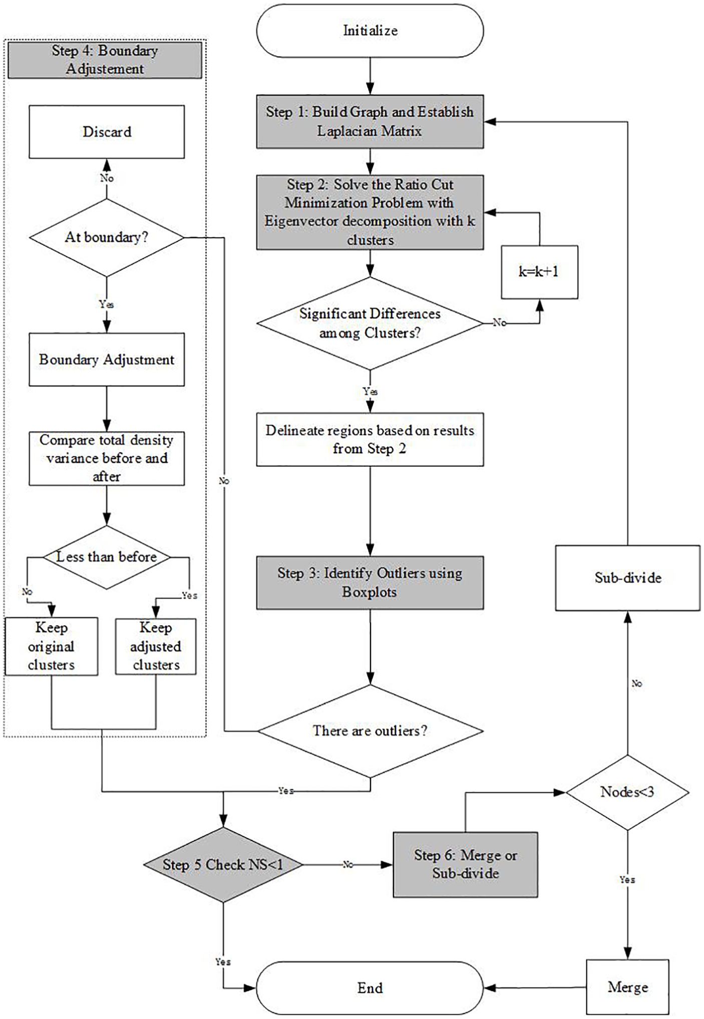
Graph-cut minimization procedure.

Step 1

Construct an undirected graph, based on the traffic network of an area of interest. Intersections are considered as nodes, while roadway sections are considered as edges. Weight $w_{ij}$ on an edge connecting two nodes is the measure of the similarity between the two nodes. Crash rate could be a candidate. Yannis et al.²¹ defined a new spatial unit based on spatial homogeneity in demographic, transport, and road safety characteristics, using the K-means algorithm. They concluded that the statistical results would be more reliable if sub-regions were more similar. Xu et al.¹⁵ proposed a zoning scheme for aggregating similar TAZs, based on the homogeneity of crash risk. Theoretically, for a pair of intersections, a longer roadway section distance indicates a lower similarity geographically, while a larger traffic volume somehow represents a higher similarity (i.e. a large attraction between two nodes). Traffic density is directly proportional to traffic volume, while inversely proportional to roadway distance. In addition, traffic density was used before in order to develop a spatial unit for regional management purposes.²³ Thus, since we want to explore the safety effects of regional traffic flow, we think that aggregating regions with traffic density is more suitable in this study. It is also interesting to partition the subject area based on other traffic flow parameters, such as speed. Those results will be reported in future research

w_{ij} = {\begin{matrix} d_{ij} = \frac{V_{ij}}{l_{ij}}, & a_{ij} = 1 \\ 0, & a_{ij} = 0 \end{matrix}

(11)

where $a_{ij}$ indicates the adjacency of intersections, $d_{ij}$ is the daily traffic density of the roadway connecting two adjacent intersections i and j, $l_{ij}$ is the roadway distance connecting adjacent intersections i and j, and $V_{ij}$ is the average daily traffic (ADT) volume.

Thus, W, D, and the Laplacian matrices can be derived for solving GC minimization.

Step 2

Compute the first k eigenvectors $v_{1}, \dots, v_{k}$ of the Laplacian matrix. Construct H as the matrix containing the vector $v_{1}, \dots, v_{k}$ as columns. For $i = 1, 2, \dots, n$ , let y be the vector corresponding to the ith row of H. Cluster the points $y_{i}, i = 1, 2, \dots, n$ , with the K-means algorithm into clusters $C_{1}, C_{2}, \dots, C_{k}$ . Then, cluster $A_{1}, \dots, A_{k}$ with $A_{i} = {j | y_{j} \in C_{i}}$ . In doing so, intersections can be properly clustered. The basic principle is that roadways in different clusters are dissimilar and those within a cluster are very similar, in terms of daily traffic density. Start from k = 2, analysis of variance (ANOVA) tests can be conducted to examine the statistical significance among clusters. When the ANOVA test rejects the null hypothesis, showing a significant difference among clusters, the initial spatial partitioning is accomplished and k sub-regions can be delineated by aggregating intersections and roadway sections within the same clusters.

Step 3

Each cluster needs to be carefully checked for extreme high or low values (i.e. extreme daily traffic density). Those outliers could be derived from malfunction or other issues of detectors, which possibly undermine the performance of spatial partitioning. Boxplot is a simple and sound way to detect extreme values.

Step 4

If there is an extreme value existing in a cluster, the corresponding edge (i.e. the roadway section) needs to be examined if it is the boundary of two nearby regions. If not, then this roadway section needs to be discarded because it may affect further sub-dividing and merging. If so, a boundary adjustment process needs to be applied, by merging the roadway section into nearby regions. Ji and Geroliminis²³ point out that boundary adjustment can refine the edges of a rough sketch to make it more distinct and clearer. The basic principle is that if the total variance of daily traffic density of two nearby regions decreases after the boundary adjustment, then the adjusted boundary will be retained; otherwise, the initial boundary will be retained.

Step 5

After boundary adjustment, each cluster will be checked for their similarities using a NS value proposed by Ji and Geroliminis²³

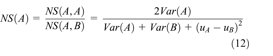
NS (A) = \frac{NS (A, A)}{NS (A, B)} = \frac{2 Var (A)}{Var (A) + Var (B) + {(u_{A} - u_{B})}^{2}}

(12)

where NS (A, B) measures the average quadratic density distance between two clusters A and B. NS (A, A) measures the average quadratic density within the cluster A. $u_{a}, u_{b}$ denote the daily traffic densities of clusters A and B.

Step 6

If a cluster has a NS less than 1, then the corresponding sub-region is considered as homogeneous in traffic density. If it has a NS greater than 1, then the number of nodes within the cluster needs to be checked. If less than 3, each node within the cluster needs to be merged into a proper nearby cluster, ensuring a lowest NS value of all clusters. If a cluster has more than three nodes, it needs to be further sub-divided based on the GC minimization method (i.e. repeat the previous steps). According to Ji and Geroliminis,²³ the average NS values of all clusters can be checked

N S_{k} = \frac{\sum_{A \in C} N S_{k} (A)}{k}

(13)

Spatial model configuration

Conventional frequency models (e.g. Poisson lognormal models) rely on a strict assumption of independence of observations, while recently spatial models have shown the superiority by incorporating spatial autocorrelation and dependency. In general, spatial crash models have shown the superiority over conventional crash models.²⁴ As for spatial crash modeling, many different models were employed before, including Poisson lognormal model, Poisson gamma model, negative binomial spatial model, Poisson lognormal spatial model, geographic weighted Poisson regression model, and Bayesian spatial varying-coefficient model.²⁵ Since the main purpose of this study is to examine the effects of traffic flow parameters rather than comparing multiple spatial models, Bayesian Poisson lognormal models with conditional autoregressive (CAR) priors are applied to analyze crash data, which has been widely applied in many different research fields such as epidemiology.²⁶

The Bayesian Poisson lognormal model with CAR prior can be presented as below

\begin{matrix} Y_{I} ~ Poisson (λ_{i}) \\ λ_{i} = E_{i} \cdot e^{(β_{0} + β_{k} X_{ik} + θ_{i} + ϕ_{i})} \end{matrix}

(14)

where $λ_{i}$ is the expected mean of crash occurrence for observation i; E is the exposure/expectation for observation i; $β_{k}$ is the parameter coefficient of kth variable; $X_{ik}$ is the kth variable for ith observation, $θ_{i}$ is the unstructured error, and $ϕ_{i}$ is the spatial correlation.

For the spatial correlation term $ϕ_{i}$ , the CAR prior can be defined as²⁷

ϕ_{i} ~ N (\bar{ϕ_{i}}, \frac{1}{τ})

(15)

\bar{ϕ_{i}} = \frac{\sum_{i \neq j} ϕ_{j} a_{ij}}{\sum_{i \neq j} a_{ij}}

(16)

τ_{i} = \frac{τ_{c}}{\sum_{i \neq j} a_{ij}}

(17)

where $a_{ij}$ is the binary entries of proximity matrix (1 represents adjacency, while 0 indicates non-adjacency). $τ_{c}$ is the precision parameter, assumed as a prior gamma distribution (0.5, 0.0005). $β_{k}$ is assumed to be a prior normal distribution (0.0, 0.001), and $θ_{i}$ is assumed to be a prior normal distribution (0, $τ_{c}$ ).

The relative risk (RR) of a sub-region can be calculated as

RR = e^{(β_{0} + β_{k} X_{ik} + θ_{i} + ϕ_{i})}

(18)

Data preparation

In this study, the central area of Kunshan, Suzhou (within the Kunshan Middle Ring Road), was of particular research interest. Overall, 5662 crash records in the year 2015 were collected from the Kunshan Police Department, containing the detailed information of drivers, roadway, and vehicles. For each record, there is a unique geographic coordinate, which can be further used for location finding in geographic information systems (GIS) map and data matching with other features (e.g. traffic flow characteristics). In order to conduct macro-level crash modeling, planning-based data including population, roadway proportion, and land use were also acquired from the Bureau of Kunshan City Planning. More importantly, 30-s-interval traffic flow data between 10 and 16 September 2015 were extracted from microwave detectors, including occupancy, speed, and traffic counts. In order to apply spatial partitioning based on the GC minimization, the daily traffic density of each roadway section was calculated and considered as the measure of traffic flow homogeneity between two intersections connected by this section. Figure 2(a) displays the subject area and detector locations.

Figure 2.

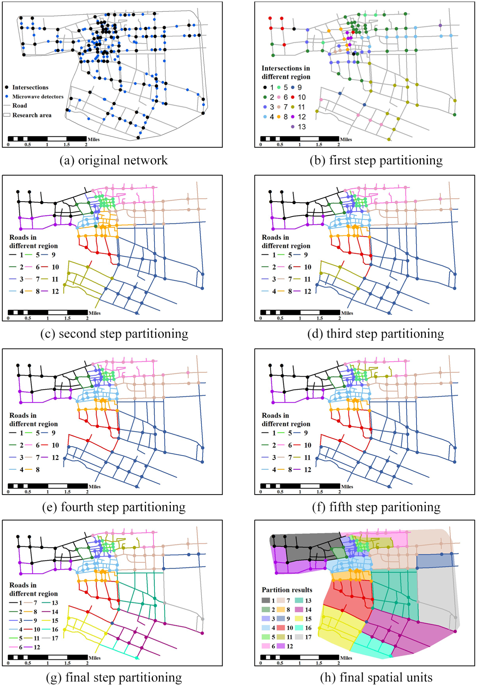
Spatial partitioning procedure based on the GC minimization method.

As for crash modeling, we selected the observed number of crashes of each sub-region as the dependent variable. We calculated the expected number of crashes for each sub-region as the crash expectation (i.e. variable E_i in equation (14)). The crash expectation of a sub-region can be derived as the total number of crashes multiplied by the proportion of its exposure, which is equal to the multiplicative of daily traffic volume, total population, and area size. The estimation of crash expectation is based on an assumption that crash risk is the same across regions. However, the relative crash risk (i.e. RR) could largely vary among different regions, intuitively. Such variations can be due to traffic, social-economic, and land use factors. Thus, 30-s microwave data were aggregated to obtain ADT and average speed of each roadway section between two intersections. Daily traffic density of each roadway section was derived by dividing ADT by section distance. Then, three spatially aggregated traffic variables (ADT, daily traffic density, and average speed) for each sub-region were calculated by averaging roadway sections within the region. Speed variance of each sub-region was also derived by calculating the variation of average speed of roadway sections. Other explanatory variables include commonly used social and lane use variables, aggregated from the planning-based data. For convenience, the spatial weight in Bayesian CAR models was considered as the adjacency-based first-order neighbors. Models were developed and compared for three spatial units (i.e. GC, TAZ, and CT), based on which variables were calculated per spatial aggregation levels. Based on the spatial partitioning procedure, there are 17 GC sub-regions. The details are discussed in section “Flow-based unit development.” All the variables available for model development are shown in Table 1. As for boundary crash assignment, the ratio of exposure method was used.²⁸ In other words, boundary crashes were all located based on the ratio of the exposure of adjacent spatial units.

Table 1.

Summary of variables and descriptive statistics.

Category	Variables	GC (N = 17)		CT (N = 44)		TAZ (N = 205)
Category	Variables	Mean	SD	Mean	SD	Mean	SD
Dependent variable	Crashes	333.06	338.09	128.68	178.73	27.62	74.52
Exposure variable	Area (square feet)	0.69	0.53	0.23	0.33	0.05	0.04
	Total population	18057.80	10891.61	6976.92	5442.81	1497.52	2267.11
	ADT	11795.97	7183.48	7353.70	7379.06	4354.79	8071.44
Roadway characteristics	Major arterial proportion (%)	28.06	22.98	22.78	24.83	14.46	27.48
	Minor arterial proportion (%)	37.19	18.09	38.84	31.78	22.66	34.19
	Local roads proportion (%)	34.75	21.96	31.56	30.37	27.26	37.94
Traffic flow	ADT	11795.97	7183.48	7353.70	7379.06	4354.79	8071.44
	Average traffic speed	43.23	21.06	32.63	22.05	29.14	24.65
	Daily traffic density	33.87	35.52	19.96	24.61	11.85	27.82
	Speed variance	10.44	9.32	26.44	33.23	25.88	29.98
	Density variance	8.28	11.25	22.54	26.12	38.28	44.52
Land use percentage	Public service	6.71	5.32	7.34	8.48	7.12	13.15
	Commercial	10.83	7.40	12.66	10.61	13.45	14.61
	Green spacing	1.96	2.76	4.30	10.24	2.64	9.96
	Industrial	6.86	10.44	6.28	16.58	8.97	19.71
	Residential	24.78	10.67	30.07	20.25	25.07	24.08
Socioeconomic variable	Floating population	269.24	192.82	104.02	123.95	22.33	32.98
	On-ground parking lots	572.94	498.80	221.36	244.27	47.51	94.89
	Underground parking lots	386.35	530.21	149.27	324.14	32.04	120.63

GC: graph cut; CT: census tract; TAZ: traffic analysis zone; ADT: average daily traffic; SD: standard deviation.

Results and discussions

Flow-based unit development

As most microwave detectors were installed along arterials in the subject area, totally 99 intersections (Figure 2(a)) were used for developing an undirected graph (i.e. 99 nodes). The GC minimization method was applied to ensure that all clusters were significantly different in daily traffic density. ANOVA tests were used to examine density difference among clusters. We started from half-cut (i.e. k = 2) and increased the number of clusters until the ANOVA null hypothesis was rejected. When k = 13, ANOVA presented a significant difference among clusters (p = 0.00012). Note that, Levene’s test and the Kolmogorov–Smirnov (K-S) test were applied to ensure equal variances of clusters and their normality.²⁹ Figure 2(b) displays the clusters of the intersections after the initial spatial partitioning. Note that there was one cluster found with only one node (i.e. one intersection). This cluster was merged into a spatially nearby cluster, and totally 12 sub-regions were delineated (Figures 2(c) and 3(a)). Then, boxplots for each cluster were drawn to identify outliers (shown in Figure 3(a)). When an outlier was found at the boundary of two adjacent regions, it was moved from the original region to a nearby region. Then, the sum of the density variance of each region was compared with the original value. When the total density variance decreased, the boundary adjustment was accepted. If not a boundary, then the outlier will be discarded in further adjustment. Figure 3(b) shows the results of boundary adjustment. After the initial boundary adjustment, the NS value of each cluster was examined. Regions 3, 6, 11, and 9 have values larger than 1. Thus, those regions were further sub-divided or merged into nearby regions. Region 3 was further sub-divided into two parts. One part had NS less than 1 and another part had only two nodes, which were merged into Region 4. Region 11 (with only two nodes) was merged into Region 9 and Region 10. After the adjustment (shown in Figures 2(e) and 3(c)), those regions had NS values less than 1. Region 6 was sub-divided into two areas using graph partitioning (k = 2). Both sub-areas had NS values less than 1. Since the nodes in original Region 11 had been merged into other regions, one sub-area was labeled as Region 11. These steps are shown in Figures 2(f) and 3(d). Region 9 was sub-divided into six parts (i.e. Regions 9, 13, 14, 15, 16, and 17). Each region was checked for their NS values. All sub-divided regions had NS value less than 1. These are shown in Figures 2(g) and 3(e). Finally, ANOVA tests were applied again to ensure significant differences among the 17 regions (Figures 2(h) and 3(f)). The average NS value is 0.8211, indicating that the proposed spatial partitioning procedure successfully lowered traffic inhomogeneity within each region, as well as enlarges the variance of traffic flow among different regions.

Figure 3.

Boxplots of clusters during the spatial partitioning procedure.

Crash model results

For the three spatial units (i.e. GC, TAZ, and CT), aggregated variables were calculated and Bayesian Poisson lognormal CAR models were developed, respectively. Correlation test and variance inflation factor (VIF) test were applied to ensure that there is no significant multi-collinearity among variables (VIF > 5) before they entered into the Bayesian CAR model. For each Bayesian CAR model, 100,000 iterations were conducted with 10,000 iterations as burn-in period. All the three models appeared to reach convergence within the simulation period. Table 2 presents the modeling results, and Figure 4 shows the observed crash number and the RR for each region based on the three spatial units.

Table 2.

Significant explanatory variables for spatial modeling for three spatial units.

Variables	GC model 2		GC model 1		CT model 2		CT model 1		TAZ model 2		TAZ model 1
Variables	Mean	SD	Mean	SD	Mean	SD	Mean	SD	Mean	SD	Mean	SD
Intercept	−2.890	0.645	0.077	0.567	−3.034	0.665	−2.993	0.385	−2.603	0.438	−2.702	0.425
Planning parameters
Minor arterials	–	–	–0.017	0.006
Local roads	–	–	–0.011	0.006					–0.001	0.005	–0.001	0.004
Public service land use					0.040	0.017	0.057	0.021	0.023	0.009	0.027	0.010
Commercial land use					0.053	0.016	0.078	0.017	0.045	0.011	0.048	0.010
Residential land use	0.061	0.006	0.059	0.014	–	–	0.027	0.009	0.028	0.007	0.031	0.009
Traffic parameters
Daily traffic density	0.011	0.020	–	–
Average traffic speed					0.022	0.006	–	–
ADT
Speed variance	0.073	0.012	–	–
Model performance
DIC	147.2		159.1		333.7		332.7		1114.9		1115.2
MAD	12.71		13.94		13.20455		12.97		4.07		4.05
MAPE	7.117626		7.59		10.26139		10.08		14.7		14.4

GC: graph cut; CT: census tract; TAZ: traffic analysis zone; SD: standard deviation; ADT: average daily traffic; DIC: deviance information criterion; MAD: mean absolute deviation; MAPE: mean absolute percentage error; model 1: original model excluding traffic flow parameters; model 2: model including traffic flow parameters.

Coefficients of significant variables are in bold.

Figure 4.

Total observed crashes and relative risk for the three spatial units.

For TAZ-based variables, residential land use was found to be correlated with underground parking lots (r = 0.65). Average speed was negatively correlated with average density (r =−0.72). TAZ is a relatively small area unit, and it could be considered as reasonable that TAZ still preserve somewhat micro-level fundamental relationships among traffic parameters. Notably, no significant correlation was found between traffic flow parameters and non-traffic factors (i.e. roadway, land use, and socioeconomic variables). Since correlated variables could raise the issue of multi-collinearity, VIF test was conducted and some variables were removed including underground parking lots and ADT. The modeling results indicate that the relationship between traffic flow parameters and regional crash risk is insignificant at TAZ level. Only planning-based variables were found significant at 95% level for both the original model and the model considering traffic flow parameters, including local roads, public land use, business land use, and residential land use. In addition, the model estimates and performance measures were almost the same for the two models. The slight differences in model estimates and performance could be attributed to the stochastic nature of Monte Carlo Markov Chain (MCMC) used by Bayesian methods. This implies that the inclusion of traffic flow parameters is unnecessary for TAZ-based models. Moreover, TAZ is a proper spatial unit for planning-based spatial modeling without potential endogeneity issues (i.e. correlation between traffic flow parameters and planning-based factors).

For CT-based variables, no significant correlation was found between traffic flow parameters and non-traffic flow parameters. Moreover, the relationship among traffic flow parameters appears to be insignificant at this regional level. This indicates that the fundamental relationship between traffic flow parameters may not always hold for spatial units at any levels. It also proves the necessity of partitioning area with similar traffic characteristics to capture macro-level traffic flow characteristics.²³ VIF test was also conducted to eliminate multi-collinearity. ADT was found to have a VIF of 9.04, which was removed before modeling crash data. For the original CT model excluding traffic flow parameters, business land use, residential land use, and public land use were found as significant. This finding is consistent with TAZ-based models. The effects of local roads became insignificant, possibly due to the aggregation (i.e. MAUP). When including traffic flow parameters, average speed, business land use, residential land use, and public land use were found as significant. Slight changes in model estimates were found for the three lane use factors, while the directions of effects remained unchanged. The overall model performances have a slight decrease (deviance information criterion (DIC), mean absolute deviation (MAD), and mean absolute percentage error (MAPE)), with the additional positive effects of average speed. However, according to previous literature,³⁰ relatively low-speed area tended to be associated with higher crash risk. Moreover, previous literature suggested the non-existence of possible linear relationship between average speed and crash risk. Thus, some potential endogeneity problem may arise that unknown factors at the CT level are correlated with average speed but not considered in the model. Thus, although the inclusion of traffic flow parameters may increase model performance, it should be treated carefully due to potential endogeneity issues. In general, the original CT-based model was well fitted.

For GC-based variables, average density is highly positively correlated with ADT (r = 0.67). Such relationship was considered as reasonable and similar to that at micro-levels. Significant correlations were found between traffic flow parameters and non-traffic parameters. ADT was positively correlated with major arterial percentage (r = 0.51) and negatively associated with green space (r = –0.59). Average speed was negatively associated with local roads percentage (r = –0.63), public land use (r = –0.51), and residential land use (r = –0.55). Note that they are not significant based on TAZ or CT units, which were developed by administrative consideration and demographics. By developing GC unit based on traffic flow homogeneity, those factors correlated with traffic flow tended to be aggregated and such correlations became significant. High correlations among roadway, land use, and socioeconomic factors were also identified. For instance, major arterial percentage was negatively associated with local roads percentage (r = –0.68). Floating population is positively associated with on-ground parking lots (r = 0.73). Residential land use is positively associated with green space (r = 0.55), floating population (r = 0.61), and underground parking lots (r = 0.83). Public land use is positively associated with commercial land use and negatively associated with underground parking lots. Such correlations could also be expected based on GC unit. Since many factors were found to be significantly correlated, multi-collinearity could be an issue that affects model estimates and performances. Multiple variables were found to have high VIF values, including underground parking lots (VIF = 21), green space (VIF = 18.8), major arterial road percentage (VIF = 11.2), and commercial land use (VIF = 7.5). Those variables were removed before entering Bayesian models. For the original Bayesian model excluding traffic flow parameters, minor arterials percentage, local roads percentage, industrial land use, and residential land use were found as significant. When considering traffic flow parameters, residential land use, speed variance, and daily traffic density were found as significant variables for the GC-based model. With the inclusion of speed variance and daily traffic density, the effects of industrial land use, local roads, and minor arterials became insignificant. Thus, the effects of traffic flow parameters (i.e. speed variance and daily traffic density) were considered to be more important at this regional level. A region with higher speed variance tends to be associated with higher regional crash risk. This is reasonable according to the previous literature.³¹ With the increase in traffic density, there is also a slight increase (b = 0.011) in crash risk. Previous literature suggests controversial findings on the relationship between traffic density and crash risk: some claimed a positive linear relationship, while others suggested a quadratic function.³² It is reasonable to expect that, at first, increased traffic density would create more interactions and thus more crash risk. While it reaches a certain level, traffic becomes too congested, resulting in fewer movement and lower crash risk. Since we only considered an average effect without regarding temporal effects, the density effect of each zone needs to be further explored in detail. The DIC, MAD, and MAPE were all significantly lower than the original model, showing it was better fitted including traffic flow effects.

Conclusion

Traffic flow parameters were found to be correlated with crash risk at micro-levels according to the previous literature.³³ The increased research attention on regional traffic management also raises an interesting question of identifying potential safety effects of traffic flow parameters at macro-levels. Moreover, it is also interesting that whether adding traffic flow parameters could also affect model performance and estimates for planning-based crash modeling. Thus, spatial crash models were developed based on three spatial units: TAZ, CT, and GC. TAZ and CT are traditional planning-based spatial units. GC is a flow-based spatial unit, which can be used for regional control purposes. To obtain GC unit, a GC minimization method was utilized to partition the central area of Kunshan, China, into sub-regions, based on the within-unit traffic density homogeneity. In order to deal with spatial dependency, Bayesian Poisson lognormal CAR models were employed. For each type of unit, two models were developed: one original model excluding traffic flow parameters and one including traffic flow parameters.

The GC-based model including traffic parameters was superior over the original one without traffic flow parameters. Moreover, it suggests significant traffic flow estimates. For the TAZ-based models, no difference in model performance was found by adding traffic flow parameters. And no significant effects of traffic flow parameters were suggested. The CT-based model including traffic parameters was found to have a slightly worse model performance than the original model. However, the effects of traffic flow parameters in the CT-based model appeared to be suspicious, possibly due to potential endogeneity issues. Thus, traffic flow parameters did not significantly improve planning-based models. However, they significantly affected crash risk for the GC-based model. Since GC units were developed for regional traffic control purposes, it can be concluded that both safety and efficiency need to be considered for regional traffic management.

In general, the safety effects of traffic flow parameters do exist at macro-levels. For planning purposes, it is unnecessary to consider traffic flow parameters as explanatory variables in macro-level crash models. However, for regional traffic management, the potential safety effects of traffic flow parameters may need to be considered and examined. This article can be considered as a preliminary study with encouraging findings for this research direction.

Admittedly, there are limitations that should be addressed. First, most traffic data were collected for arterial roads, where microwave detectors are installed. Thus, only those roads were used for spatial partitioning. Limited by the sparsity of microwave data and the size of the subject area, only 17 GC zones were finally delineated, which possibly raise overfitting issue. Nonetheless, the intent of the modeling is not for prediction but identifying model effects. Moreover, Bayesian CAR models were introduced to deal with the issue and the coefficients were assumed to follow prior normal distributions which can be considered as the equivalence of L₂ regularization.³⁴ Second, spatial and temporal heterogeneity were not considered in this study. Spatial heterogeneity had been discussed in the previous literature.¹⁶ It could be examined in the future, especially for the effect of multiple traffic flow parameters. Moreover, since GC unit is defined based on traffic flow data instead of planning data, temporal heterogeneity can also be discussed in the future. Also, other traffic flow parameters can be attempted for spatial portioning, instead of traffic density. Third, only several simple aggregated traffic parameters were considered in the study. It is interesting to extract other features of traffic flow (e.g. the features of macroscopic fundamental diagram) and examine their possible effects on safety. In addition, other spatial models (e.g. simultaneous autoregressive model) can be applied in the future to identify those effects. Finally, boundary crash data assignment is an important issue that needs to be further examined. Currently, a previous method was used in this study. However, according to recent literature,³⁵ there have been many different methods dealing with the boundary issue. We recommend that future studies can be focused on these research topics.

Footnotes

Handling Editor: Jiangchen Li

Declaration of conflicting interests

The author(s) declared no potential conflicts of interest with respect to the research, authorship, and/or publication of this article.

Funding

The author(s) disclosed receipt of the following financial support for the research, authorship, and/or publication of this article: This research was supported by the National Natural Science Foundation of China (nos 51508093 and 51608114) and the Fundamental Research Funds for the Central Universities (no. 2242018K40008).

ORCID iD

Chen Wang

References

Daganzo

CF.

Urban gridlock: macroscopic modeling and mitigation approaches. Transp Res Part B 2007; 41: 49–62.

Geroliminis

Haddad

Ramezani

Optimal perimeter control for two urban regions with macroscopic fundamental diagrams: a model predictive approach. IEEE Trans Intell Transp Syst 2013; 14: 348–359.

Kouvelas

Saeedmanesh

Geroliminis

Enhancing model-based feedback perimeter control with data-driven online adaptive optimization. Transp Res Part B 2017; 96: 26–45.

Zhang

Parr

Jiang

et al . Optimization model for regional evacuation transportation system using macroscopic productivity function. Transp Res Part B 2015; 81: 616–630.

Yildirimoglu

Ramezani

Geroliminis

Equilibrium analysis and route guidance in large-scale networks with MFD dynamics. In: 21st international symposium on transportation and traffic theory, Kobe, Japan, 5–7 August 2015, pp.185–204. New York: Elsevier.

Zhang

Path optimization of taxi carpooling. PLoS ONE 2018; 13: e0203221.

Strating

Coordinated signal control for urban networks by using MFD. MSc Thesis, Civil Engineering, Delft University of Technology, Delft, 2010.

Chu Tian

Wang

. Traffic signal control with macroscopic fundamental diagrams. In: IEEE American Control Conference (ACC), Chicago, IL, 1–3 July 2015. New York: IEEE.

Hao

Wang

et al . Developing a coordinated signal control system for urban ring road under the vehicle-infrastructure connected environment. IEEE Access 2018; 6: 52471–52478.

10.

Marchesini

Weijermars

. The relationship between road safety and congestion on motorways (R-2010-12). Leidschendam: SWOV Publication.

11.

Noland

Quddus

MA.

A spatial disaggregate analysis of road casualties in England. Accid Anal Prev 2004; 36(6): 973–984.

12.

Haynes

Jones

Kennedy

et al . District variations in road curvature in England and Wales and their association with road-traffic crashes. Environment and Planning A 2007; 39(5): 1222–1237.

13.

Wang

Quddus

Ryley

et al . Spatial models in transport: a review and assessment of methodological issues. In: 91st annual meeting of the transportation research board, Washington, DC, 22–26 January 2012. US: National Research Council.

14.

Abdel-Aty

Lee

Siddiqui

et al . Geographical unit based analysis in the context of transportation safety planning. Transport Res Part A Policy Pract 2013; 49: 62–75.

15.

Huang

Dong

et al . Sensitivity analysis in the context of regional safety modeling: identifying and assessing the modifiable areal unit problem. Accid Anal Prev 2014; 70: 110–120.

16.

Amoh-Gyimah

Saberi

Sarvi

The effect of variations in spatial units on unobserved heterogeneity in macroscopic crash models. Anal Meth Accid Res 2017; 13: 28–51.

17.

Lee

Abdel-Aty

Jiang

Development of zone system for macro-level traffic safety analysis. J Transp Geogr 2014; 38: 13–21.

18.

Huang

Song

et al . Macro and micro models for zonal crash prediction with application in hot zones identification. J Transp Geogr 2016; 54: 248–256.

19.

Huang

Dong

et al . Revisiting crash spatial heterogeneity: a Bayesian spatially varying coefficients approach. Accid Anal Prev 2017; 98: 330–337.

20.

Martin

Extending the automated zoning procedure to reconcile incompatible zoning systems. Int J Geogr Inform Sci 2003; 17: 181–196.

21.

Yannis

Papadimitriou

Aotoniou

Multilevel modeling for the regional effect of enforcement on road accidents. Accid Anal Prev 2007; 39: 818–825.

22.

Guo

Wang

Automatic region building for spatial analysis. Trans GIS 2011; 15: 29–45.

23.

Geroliminis

On the spatial partitioning of urban transportation networks. Transp Res Part B 2012; 46: 1639–1656.

24.

Mannering

Bhat

CR.

Analytic methods in accident research: methodological frontier and future directions. Anal Meth Accid Res 2014; 1: 1–22.

25.

Cheng

Singh

Dasu

et al . Comparison of multivariate Poisson lognormal spatial and temporal crash models to identify hot spots of intersections based on crash types. Accid Anal Prev 2017; 99: 330–341.

26.

Wakefield

Best

Waller

. Bayesian approaches to disease mapping. In: Elliot

Wakefield

Best

et al . (eds) Spatial epidemiology: methods and applications. Oxford: Oxford University Press, pp. 104–127.

27.

Besag

York

Molli

EA.

Bayesian image restoration with two applications in spatial statistics. Annu Inst Stat Math 1991; 43: 1–59.

28.

Wei

Boundary effects in developing macro-level CPMs: a case study of city of Ottawa. Vancouver, BC, Canada: The University of British Columbia, 2010.

29.

Durrett

Probability: theory and examples. Cambridge: Cambridge University Press, 2010.

30.

. Real-time estimation of freeway accident likelihood. In: Proceedings of the 80th TRB annual meeting, Washington, DC, 22–26 January 2001. US: National Research Council.

31.

Abdel-Aty

Pande

Identifying crash propensity using specific traffic speed conditions. J Safety Res 2005; 36: 97–108.

32.

Lee

Saccomanno

Hellinga

Analysis of crash precursors on instrumented freeways. Transport Res Record 2002; 1784: 1–8.

33.

Wang

Liu

et al . Calibration of crash risk models on freeways with limited real-time traffic data using Bayesian meta-analysis and Bayesian inference approach. Accid Anal Prev 2015; 85: 207–218.

34.

Bishop

Pattern recognition and machine learning. London: Springer, 2011.

35.

Zhai

Huang

Gao

et al . Boundary crash data assignment in zonal safety analysis: an iterative approach based on data augmentation and Bayesian spatial model. Accid Anal Prev 2018; 121: 231–237.

On the safety effects of spatially aggregated traffic flow parameters at macro-levels

Abstract

Keywords

Introduction

Methodology

Flow-based spatial unit development

GC minimization problem

Procedure for flow-based unit development

Step 1

Step 2

Step 3

Step 4

Step 5

Step 6

Spatial model configuration

Data preparation

Results and discussions

Flow-based unit development

Crash model results

Conclusion

Footnotes

Declaration of conflicting interests

Funding

ORCID iD

References