Sage Journals: Discover world-class research

Abstract

Speed illusion is the leading contributing factor to traffic accidents in highway tunnels. This study aimed to estimate the influence of visual information at different scales and frequencies on drivers’ visual perception and driving safety in highway tunnels. The speed perception of drivers was measured using the stimulus of subjectively equivalent speeds as an index. Thirty drivers were recruited to conduct a psychophysical experiment on speed perception using a driving simulator. The large-, medium- and small-scale visual information in a frequency range of 0.1–32 Hz were used in the experimental scene to generate scenes for comparison. The results show that high-frequency visual information (2–32 Hz) might lead to driver overestimation of vehicle speed in tunnels, while medium-frequency (0.4–1 Hz) and low-frequency (0.1–0.2 Hz) visual information contribute to speed underestimation. The medium-scale information had the largest speed overestimation effect, followed by large- and small-scale information (significant differences of 2–8 Hz). Medium-scale visual information below 8 Hz had the lowest degree of dispersion of speed perception. Therefore, the use of integrated high-frequency, medium-scale visual information and medium-frequency, large- and small-scale visual information is suggested to reduce the speed illusion of drivers and ensure driving safety.

Keywords

Multiscale multifrequency driving safety highway tunnel speed perception visual information

Introduction

A driver obtains traffic environment information by sight and then makes judgements, decisions and reactions regarding any potential risk. Statistic surveys from Highway Traffic Police Department in China reveal that 38% of traffic accidents are closely related to drivers’ incorrect estimation of their driving speed.¹ A reduction in speed illusion of drivers can therefore significantly reduce acts of speeding and enhance road traffic safety.

China has the largest number of highway tunnels in the world. As of 2015, the country had 14,006 highway tunnels, with a total length of 12,683 km.² Highway tunnels are accident-prone locations, often with heavy casualties, with statistics showing that the average rate of traffic accidents in a highway tunnel section is approximately five times higher than that in an open section.³ The characteristics of low luminance, monotonous environment and semi-enclosed shape in the middle of highway tunnels make them a weak visual reference system. This weakness leads to deficiency of the visual reference system for drivers and thus reduces their perception of their actual driving speed, resulting in an extremely high risk of overspeeding and rear-end accidents.⁴ A domestic survey shows that as many as 40% of the accidents occurring along the Yuyuan highway and Shangsan highway are due to excessive driving speed.⁵ However, close links exist between real speed and perceived speed, namely, the increase in a driver’s perceived speed is approximately twice the decrease in real speed.⁶ Therefore, it is worth exploring an effective way to control driving speed in highway tunnels via identifying ways to increase a driver’s perceived speed, lowering the real speed and ultimately reducing the accident rate and intensity.

This study assesses the effect of visual information on drivers’ speed perception at various scales and frequencies in highway tunnels. The optimal combination of scale and frequency of traffic facilities is explored to achieve the best speed control effect and thus improve driving safety in highway tunnels.

Literature review

Tunnel lighting is a way to enhance drivers’ speed perception. Human speed perception is modulated by a range of stimulus attributes, such as the contrast and luminance of environment.^7–9 At slow speeds, a reduction in the contrast leads to an underestimation of velocity, but conversely, objects in the environment can appear to move more quickly at higher speeds (>8 Hz).^8,9 In addition, considering the luminance factors, low contrast stimuli are perceptually biased at both low (2.5 cd/m²) and high (25 cd/m²) luminance levels such that they appear to be slower at low (<8 Hz) speeds but faster at high (16 Hz) speeds,¹⁰ which can make things appear to move slower or faster depending on ambient lighting, contrast and temporal frequency.¹¹ Horswill and Plooy investigated the effect of reducing image contrast on speed perception using a video-based driving simulator. Reduced contrast was found to possibly make speeds difficult to distinguish and appear slower.¹² For the contrast and luminance in a tunnel, good general lighting of tunnel can make drivers feel more comfortable and safe, and lights will increase the safety distance between oncoming vehicles. In addition to lighting, good contrast should exist between colour of the wall and road surface.¹³ Buchner et al.¹⁴ indicated that the perceived car distance increases as the tunnel luminance decreases. Kircher and Ahlstrom¹⁵ conducted a parametric study of different levels of brightness and different colours on sidewalls and suggested that light-coloured sidewalls induce a safer driving environment in tunnels.

The Chinese industry standard ‘Guidelines for design of lighting of highway tunnels’¹⁶ stipulates that the lengths of highway and first-class highway tunnels should be longer than 200 m and that lighting systems should be set up, resulting in large energy consumption in low-traffic areas, especially in western China. In these areas, standard lights are usually installed, but the energy consumption is costly. As a result, lights are only partially functional. For example, the lighting rate is only 40% of the national standard in Qinling Zhongnanshan tunnel, Shanxi province, and the day lighting rate of remaining extra-long tunnel in Shanxi province can reach only 30% of the national standard.¹⁷ This is also considered to be one of the main reasons for traffic accidents during tunnel–luminance transitions.

The luminance in the practical operation of highway-tunnel lighting is significantly lower than the design standard, which is at the expense of traffic safety. To strike a balance between traffic safety and energy conservation, quantitative investigations on the relationship between tunnel lighting level and speed perception must be carried out.

Regarding the application of traffic facilities for visual speed control, Manser and Hancock¹⁸ analysed the effects of decreased-, increased- and constant-width vertical segments along tunnel sidewall on drivers’ speed perception via simulation experiments. The results indicate that drivers gradually decreased speed as the width visual pattern decreased and increased speed as the width visual pattern increased. Liu¹⁹ investigated the influence of edge rate on speed control via psychophysical experiments, discovering that drivers might underestimate their driving speed for edge rates smaller than 2 Hz or larger than 32 Hz. However, speed overestimation occurred for edge rates in a range of 4–16 Hz. Song et al.²⁰ and Wu et al.²¹ designed tunnel sidewall markings with various patterns, colours and spacings. The simulations showed that use of the colour blue in tunnels might reduce driver fatigue. Moreover, a spacing of 10–20 m between markings could effectively improve drivers’ sense of their speed. Wan et al.^22,23 investigated the effect of high-frequency visual information and a combination of high- and medium-frequency visual information on the sense of speed and reaction time of drivers under different levels of illumination (100%, 50% and 25% standard illumination) in tunnels, specifically observing how colours and temporal frequencies affected a driver’s speed perception under the low-luminance conditions of tunnels. The results show that good illumination conditions and multifrequency visual information were beneficial in enhancing driver sensitivity to driving speed and preventing unconscious acceleration when driving in the middle of tunnels at high speeds. In addition, the subjects made the highest speed overestimations and could make easy speed judgements with a red–white combined sidewall marking.

Driving simulator experiments have been widely applied in driving behaviour studies as well as speed perception studies.^18,20–23 Although most simulators involve a flat, two-dimensional (2D) display and not a three-dimensional (3D) display, the simulated speeds are highly correlated with real-world performance data,²⁴ and during driving, a simulator can perceive the impact of contrast reduction on speed perception.¹² The presence of stereoscopic cues regarding motion in depth can significantly enhance the precision of speed judgements; however, the accuracy of speed judgements is unaffected by it, with satisfactory performance being achieved under the 2D condition. Using a driving simulator containing stereoscopic cues can lead to better simulation of a speed perception experiment.²⁵

The practical traffic environment always involves visual information at multiple frequencies: high-frequency visual information, such as slow-down markers and guardrails on the road; low-frequency visual information, such as the delineator, lane lines and roadside trees; and large-scale road landscape information, such as distant houses, mountains and so forth. The landscape information in the highway environment is always used as an external source by drivers to perceive their driving speed,²⁶ enabling them to reduce their speed and increase speed control, with the presence of more references resulting in slower speeds.²⁷

Overall, the low-luminance driving environment in China’s highway tunnels is ubiquitous. Low illumination can trick drivers into thinking that their speeds are under the limitation, resulting in them driving faster.²⁸ This outcome leads to increased speeding behaviour, which is one of the major causes of highway-tunnel accidents. Therefore, the contradiction between energy-saving lighting systems and traffic safety in highway tunnels is a major challenge. Current research on visual illusion markings suggests that high-frequency visual information makes a driver overestimate his own driving speed, while low-frequency visual information may induce a speed underestimation.^19,20,23 Thus, high-frequency pavement markings have been used widely to enhance the speed perception of drivers on highways. However, quantitative investigation of the influence of visual information with frequency and scale on the occurrence of driver visual illusion in tunnels is limited. The current improvement measures for lighting conditions in tunnels have proven uneconomical. They are not applicable to tunnels with small traffic volumes in China and are confined by natural environment and economic conditions. Meanwhile, it is difficult for drivers to identify common traffic facilities in the traffic environment (with low luminance and contrast), which limits their effects on traffic safety. Therefore, a reasonable evaluation of the visual illusion level of drivers in a tunnel as well as the low-cost improvement measures is the key to achieving a balance between traffic safety and energy-saving lighting. This study quantitatively explores visual illusion degree of drivers in a tunnel using a driving simulator. To achieve this objective, the following questions were addressed:

What index is needed to reasonably evaluate the influence of tunnel patterns on visual illusion and driving behaviour of drivers?

What is the quantitative relation between driver visual illusion and visual information at different scales, frequencies and levels of luminance?

Experimental layout and data collection

High risk and operational difficulty limit real vehicle testing in the middle of highway tunnels; moreover, tunnel lighting adjustment and traffic marker arrangement depend on traffic flow, cost and management. Hence, this study adopted the 3ds Max software to establish driving model and E-prime-based software to conduct psychophysical tests of speed perception. The test data were then statistically analysed using Origin version 8.0 and SPSS version 20.0 (SPSS, IL, USA).

Driving simulator

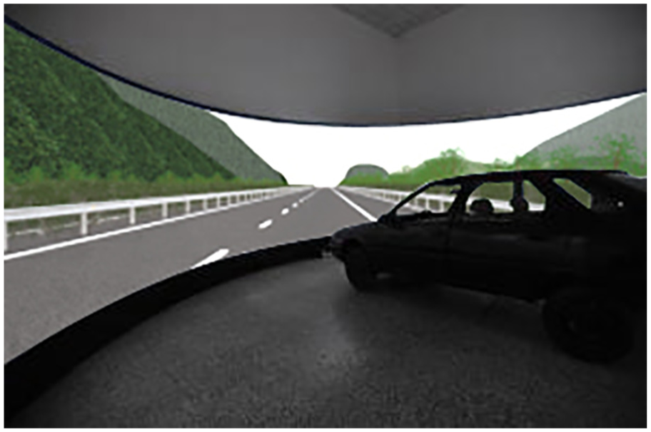
The Wuhan University of Technology, Intelligent Transport System, High Definition (WUTITS-HD) driving simulator from Wuhan University of Technology was used to perform the driving simulation. This simulator is part of a new generation of vehicle driving simulators independently developed by Wuhan University of Technology. It can be applied to study issues related to road traffic safety under controlled experimental conditions. These issues include driver behaviour analysis, automatic driving simulation and traffic guidance design. The driving simulator details are given in Figure 1.

Figure 1.

Advanced moving base simulator.

Test method and procedure

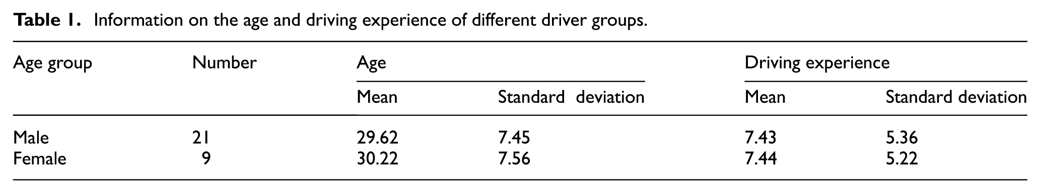
A total of 30 drivers were tested. According to the ratio of male drivers to female drivers in China of 7:3, the number of the former was 21 and that of the latter was 9. Twelve drivers were 20–25 years old, five were 26–30 years old, five were 31–35 years old, four were 36–40 years old and four were 41–45 years old (mean value: 29.8; standard deviation: 7.34). All the participants had more than 3 years of driving experience. All have good vision and experience driving in highway tunnels. More details regarding the age and driving experience of drivers are shown in Table 1.

Table 1.

Information on the age and driving experience of different driver groups.

Age group	Number	Age		Driving experience
Age group	Number	Mean	Standard deviation	Mean	Standard deviation
Male	21	29.62	7.45	7.43	5.36
Female	9	30.22	7.56	7.44	5.22

The method of limits, also called the method of minimal change, is a direct method for measuring the threshold.²⁹ This method is used to find the instantaneous transition point or threshold position from one reaction to another by changing the stimulus (in increasing or decreasing order) in small, equal intervals. The method of limits was used in this study to determine stimulus of subjectively equal speed (SSES).³⁰

Two speed stimuli in increasing and decreasing order, respectively, were adopted in the test. As shown in Figure 2, V_std is the speed in standard scene, V_cmpi is the speed in comparison scene i and a is the minimum interval. When the minimum interval a < 0, speed stimuli in the comparison scene are in decreasing order. When a > 0, the speed stimuli are in increasing order, as shown in Figure 2. Once a subject encountered opposite stimulus, speed in the comparison scene was SSES, such as that in increasing order, that is, a > 0, if the subject felt that V_cmp1 < V_std and V_cmp2 < V_std in scene 1 and scene 2, respectively. However, the subject experienced V_cmp3 > V_std when switched to scene 3; hence, SSES = V_cmp3. To maintain a balance between the number of experiments and the minimum change in perception speed, the speed range in the comparison scene was V_cmpi = [V_std – 20, V_std + 20], a = 2.5 km/h.²² Both training effect and fatigue effect were caused by performing the same experiments for a long time. If experiments were performed using the increasing or decreasing sequence of speed changes all the time, subjects could easily become more familiar with the experimental scenarios, causing an increase in practice error and fatigue error. The ABBA method²⁹ was used in this study to correct for these errors. A denotes the speed stimulus in an increasing sequence, while B denotes the stimulus in a decreasing sequence. The tests were carried out in a sequence of ABBA. As a result, each test has 30 × 4 = 120 sample points. The E-prime software was used to conduct the aforementioned process.

Figure 2.

SSES detection method.

The detailed operation steps are as follows:

A laptop computer was used to run E-prime software in simulator. The video simulation test was started by pressing Q on keyboard, after which the video started playing on the simulator screen.

Before the formal test, the subjects had to become familiar with the test for 10–15 min with the help of operators and perform three pre-experiments randomly. The pre-experiment scene was the same as formal experiment scene. However, the comparison scene of pre-experiment had certain scale information appearing at a certain frequency at random. The pre-experiment tests only whether the subjects are familiar with experimental operation.

Before starting the comparison video, a preparation time of 3 s was reserved for each subject.

Each subject was required to face towards the road ahead and make judgements regarding the speed of comparison stimulus relative to the standard stimulus as soon as possible (within 10 s).

If a subject felt that perceived speed in the left video screen was higher than that in the right video screen, the left button of handle was pressed. In contrast, if perceived speed in the right video screen was higher than that in the left video screen, the right button of handle was pressed.

After each increasing or decreasing stimulus test, scenery pictures of 30 s were played to offer subjects a period of rest.

Visual information includes three scales, namely, large-scale information, medium-scale information and small-scale information. Each scale of visual information changes from 0.1 to 32 Hz under standard illumination. The given visual information at a certain frequency was used as a set of experiments. After each test with certain visual information at a certain frequency, the test was stopped for a 3-min break. For example, the test ends for 3 min after the test of small-scale markings at 0.1 Hz under standard luminance ends but before the test of small-scale markings at 0.2 Hz under standard luminance begins.

E-prime software was used to output the test data and to calculate and analyse SSES.

The presentation of each clip of motion occurred simultaneously, the stimulus duration was 10 s and each subject was required to make a judgement within 10 s. Each scene used the same straight stretch of road and started at the same location each time. Only the speed and traffic markings of compared experiment scenes served as stimuli.

Validation of simulation accuracy

Compared with field test, the simulation test had a certain level of distortion. Experiments were carried out in this study to examine the precision of the simulation test compared with field test (both involved common sections of highways). Wan et al.²² analysed the difference between real speed in the low-luminance tunnel field and perceived speed by the tunnel model in driving simulation; the difference was approximately 30%, and the accuracy often failed to meet the requirements. Therefore, this study chose a common section of highways as standard stimulus. The field test and simulation scenes are shown in Figure 2; the field test scene is shown as the standard scene, while the simulation scenes are shown as the comparison scenes. A driving speed of 74 km/h (measured by flash frequency of the lane edge line) was taken in field test. The speed in simulation test was V_cmpi = [54, 94] km/h, and the minimum interval was a = 2.5 km/h.²² Twenty subjects participated in the calibration experiment. The SSES measured via the method of limits was 75.13 km/h. The error between the speed predicted by proposed model and measured result was −1.52%. The results of one-sample t tests showed that p = 0.083 > 0.05. The accuracy of the model was proven provided that no significant difference between simulator model and field test existed. Thus, the video of the simulation model was set as the standard stimulus, and then SSES experimental results were multiplied by 98.48% (=100% – 1.52%).

Speed perception test regarding visual information at different scales

Design of traffic information at different scales

To study the influence of visual information at different scales and frequencies on the visual illusion of drivers in semi-enclosed tunnels, visual information at large, medium and small scales was designed according to ‘Specifications for design of highway tunnel’.³¹ The design details are shown in Table 2 and Figures 3 –5.

Table 2.

Design of visual information at different scales in the middle of highway tunnels.

Type of visual information	Facilities	Size: length × width (m)	Type of reflective material	Colour
Large scale	Semi-annular markings; transverse pavement markings (forming a closed shape)	Semi-annular markings: 0.5 (width); transverse pavement markings: 0.5 × 0.5; height: 6.89	Thermoplastic markings; all-weather reflective markings	White
Medium scale	Vertical markings	Kerb: 0.2 (width); maintaining roadway: 0.3 (width); height: 0.5	Thermoplastic markings	Red and white
Small scale	Delineator on the sidewall	0.16 × 0.04	High-strength reflecting film	Yellow on the left and white on the right

Because the height ratio of different-scale visual information was 6.89:0.5:0.16 = 43.0625:3.125:1, the scales of tunnel’s visual information were divided into large, medium and small scale.

Figure 3.

Schematic of large-scale markings in the middle of highway tunnels: (a) lateral view and (b) plan view.

Figure 4.

Schematic of medium-scale markings in the middle of highway tunnels (lateral view).

Figure 5.

Schematic of small-scale markings in the middle of highway tunnels (lateral view).

The drivers’ fixation point in tunnel was mainly concentrated in the following places:³² (1) in front of the vehicles and the roads far ahead, which is the main visual area near the centre; (2) the tunnel wall on the left and right side, the road shoulder, which is the main visual area of left side and right side; (3) above the tunnel, which is where the sight ended and (4) the near roads in front of the car. Different scales of visual information were divided based on the height of facility in the driver’s field of vision. The height of large-scale information occupied most of the driver’s vertical field of view, including mostly above the tunnel and the tunnel wall on the left- and right-side part of the roads far ahead. The height of medium scale information occupied about half of the driver’s vertical field of view, including most of the tunnel wall on the left- and right-side part of the roads far ahead. The height of small-scale information occupied less than one-third of the driver’s vertical field of view, including only part of the tunnel wall and the roads far ahead.

Test design

Video simulation tests were carried out to investigate the speed underestimation phenomenon in the middle of tunnels. The test scenes were classified into standard test scenes and comparison test scenes. A standard scene was defined as the basic road traffic environment along a highway. According to the ‘Technical standard of highway engineering’,³³ for a design speed of 80 km/h, a central separate belt width of 2 m and a lane width of 3.75 m, the left and right hard shoulder widths should be 0.75 and 2.5 m, respectively. The comparison scene depicts the traffic environment in the middle of a highway tunnel. According to ‘Specifications for design of highway tunnel’,³¹ the highway tunnel should be designed as a separate independent double hole with a construction gauge height of 5 m and side road height of 0.75 m. For a given design speed of 80 km/h, the single lane width was taken as 3.75 m, left lane width as 0.50 m and right lane width as 0.75 m.

The simulation test used the standard highway driving video as standard stimulus. The speed of standard stimulus was 80 km/h, the speed of comparison stimulus varied over a range of 50–110 km/h and the speed interval was taken as 2.5 km/h. The standard luminance corresponds to JTG/T D70/2-01-2014:2014.¹⁶ High-pressure sodium (HPS) of 100 W was arranged bilaterally and symmetrically with an interval of 10 m. The luminous efficacy was 110 lm/W, colour temperature was 1800 K and the average pavement luminance was 4.5 cd/m². Two headlights were set for the lighting effect. The power of two headlights was 60 W, and the colour temperature was 1800 K. The luminance level was significantly higher on the lighted surface of retroreflective traffic patterns (delineators and traffic markings) than on the nonlighted areas.

The standard scene was unchanged, while in the contrast tests, the spacing between traffic markings was changed with a frequency range of 0.1–32 Hz (for a speed of 80 km/h). The compared experimental scenes were as follows:

Scene 1: No traffic markings in the middle of highway tunnels, as shown in Figure 6(a);

Scene 2: Large-scale markings (semi-annular markings) and transverse pavement markings (as listed in Table 2) with a range of 0.1–32 Hz, as shown in Figure 6(b);

Scene 3: Medium-scale markings (vertical markings in Table 2) with a range of 0.1–32 Hz, as shown in Figure 6(c);

Scene 4: Small-scale markings (delineator in Table 2) with a range of 0.1–32 Hz, as shown in Figure 6(d).

Figure 6.

Comparison of experimental scenes: (a) scene 1, (b) scene 2, (c) scene 3 and (d) scene 4.

Test results and analysis

The quantity and distribution of SSESs under visual information at different scales and frequencies were obtained by the method of limits. The results are shown in Table 3 and Figure 7. For tunnels without any visual reference system (i.e. no large-, medium- or low-scale visual information), SSES = 97.08 ± 10.12 km/h, with speed underestimated by up to 21.35%.

Table 3.

Comparison of SSESs.

Frequency (Hz)	Large scale		Medium scale		Small scale
Frequency (Hz)	SSES (km/h)	Speed illusion (%)	SSES (km/h)	Speed illusion (%)	SSES (km/h)	Speed illusion (%)
0.1	96.38 ± 8.47	−20.48	96.75 ± 7.62	−20.94	96.88 ± 9.60	−21.10
0.2	94.29 ± 10.14	−17.86	95.42 ± 6.80	−19.28	95.00 ± 8.17	−18.75
0.4	87.96 ± 6.30	−9.95	88.00 ± 5.42	−10.00	91.08 ± 7.03	−13.85
0.6	84.50 ± 4.99	−5.63	85.38 ± 4.86	−6.73	88.75 ± 6.91	−10.94
0.8	84.08 ± 4.94	−5.10	84.13 ± 5.98	−5.23	84.71 ± 4.65	−5.89
1	83.46 ± 4.65	−4.33	83.29 ± 4.35	−4.11	82.50 ± 5.19	−3.13
2	76.67 ± 3.98	4.16	82.29 ± 3.72	−2.86	80.79 ± 3.52	−0.99
4	68.38 ± 4.31	14.53	71.63 ± 3.41	10.46	75.92 ± 4.53	1.97
8	60.33 ± 3.64	24.58	64.42 ± 2.78	19.48	70.22 ± 3.14	8.59
12	59.38 ± 4.41	25.78	57.29 ± 3.26	28.39	66.75 ± 4.28	10.31
16	60.21 ± 5.41	27.86	53.88 ± 4.33	32.65	69.75 ± 5.04	12.81
32	64.38 ± 7.26	20.63	52.17 ± 3.81	34.79	71.38 ± 4.35	10.78

Speed illusion = (speed in the standard scene – SSES) / speed in the standard scene.²³‘–’ in speed illusion denotes speed underestimation. ‘±’ in SSES represents standard deviation.

Figure 7.

Distribution of SSESs: (a) the distribution of SSES at large-scale markings, (b) the distribution of SSES at medium-scale markings and (c) the distribution of SSES at small-scale markings.

After taking the logarithm of frequency, the distribution of SSESs is as shown in Figure 7.

The results in Table 3 and Figure 7 reveal the following:

The visual information in a range of 0.1–1 Hz causes significant speed underestimation, the magnitude and variance of which shows a decreasing trend with increase in frequency. The speed underestimation effect due to small-scale visual information (SSES_s–0.4 = 91.08 km/h, SSES_s–0.6 = 88.75 km/h) for frequencies from 0.4–0.6 Hz was better than that due to the large-scale (SSES_L–0.4 = 87.96 km/h, SSES_L–0.6 = 84.50 km/h) and medium-scale (SSES_M–0.4 = 88.00 km/h, SSES_M–0.6 = 85.38 km/h) visual information.

For visual information corresponding to 2–8 Hz, the large-scale visual information yielded the largest speed overestimation, followed by medium-scale and small-scale information (F(2, 1077) = 88.93, p < 0.01). The medium-scale information at high frequencies of 2–32 Hz had the lowest degree of speed perception dispersion. The medium-scale information below 8 Hz had the lowest degree of dispersion, that is, ±2.78 km/h.

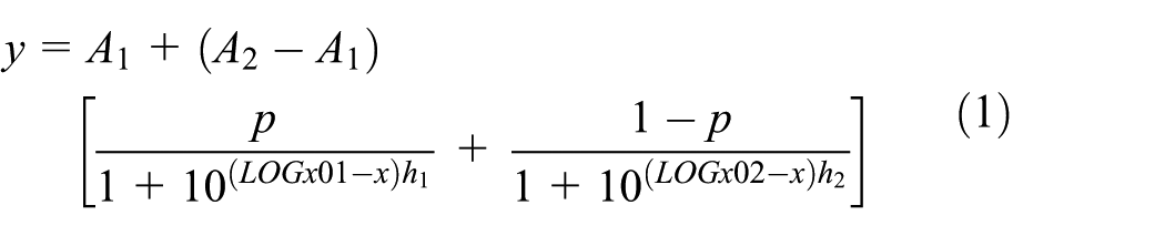
F Mannering³⁴ showed that the larger the dispersion degree of perceived speed, the higher the accident rate. Therefore, the large-, medium- and small-scale visual information under 8 Hz had the lowest perceived speeds with a low degree of dispersion. To study the change in SSES at low frequency (0.1–0.2 Hz), medium frequency (0.4–1 Hz) and high frequency (2–32 Hz), a double S-type function with multiple mutations was selected. The BiDoseResp function was used to fit SSESs of large-, medium- and small-scale information at different frequencies according to formula (1), as shown in Figure 8

\begin{matrix} y = A_{1} + (A_{2} - A_{1}) \\ [\frac{p}{1 + 10^{(LOGx 01 - x) h_{1}}} + \frac{1 - p}{1 + 10^{(LOGx 02 - x) h_{2}}}] \end{matrix}

(1)

Figure 8.

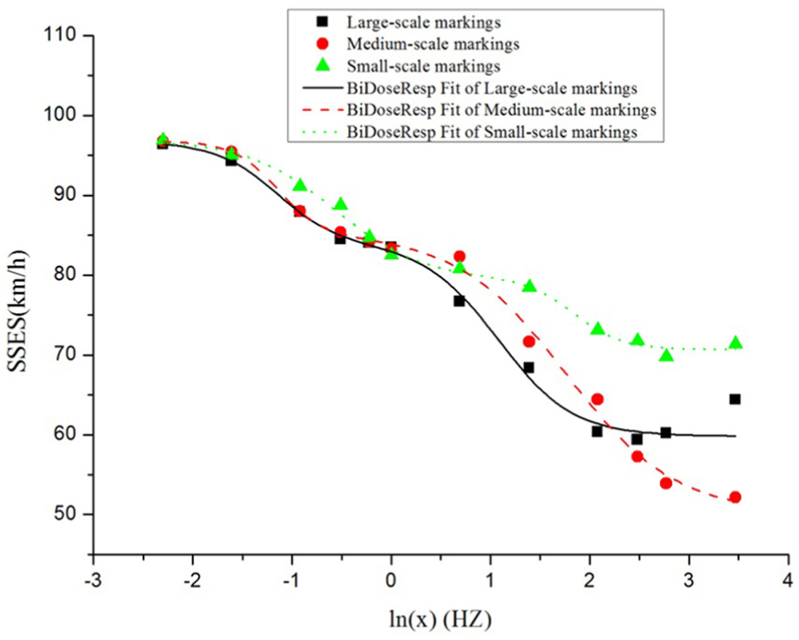
BiDoseResp fit of SSESs.

The fitting parameters are shown in Table 4.

Table 4.

The fitting results.

	A ₁	A ₂	LOGx01	LOGx02	h ₁	h ₂	p	R ²	x ₁	x ₂
Large scale	60.867	96.663	−1.153	1.033	−1.424	−1.225	0.357	0.976	0.316	2.809
Medium scale	50.159	96.812	−1.146	1.758	−1.957	−0.788	0.249	0.992	0.317	5.800
Small scale	70.689	96.879	−0.562	1.845	−0.979	−1.812	0.666	0.990	0.570	6.328

The factors LOGx01 and LOGx02 indicate the first and second tipping points of the SSES gradient, respectively, and x₁ and x₂ are frequencies after conversion, respectively. Based on x₁ and x₂, the changing curve of SSES can be separated into three sections: SSES of large and medium scales will undergo the first mutation at low frequency, SSES of small-scale mutates at medium frequency and the second mutations of all scales, that is, speed estimation changing from underestimation to overestimation, occur at high frequency. Therefore, distances of information appearing in the tunnel should be shortened as visual information scale shrinks. In other words, the denser the information is, the greater influence it can have on SSES.

To examine the difference between any two mean values, Student–Newman–Keuls (SNK) method was used in terms of a checking statistic Q (also known as Q test), which is a method for effectively dividing a similarity subset. The SNK method demonstrates only the difference without providing the value of p.

Tables 3 and 5 show that for a 100% standard lighting tunnel, the following is true:

The results from one-way analysis of variance (ANOVA) show that for low-frequency visual information (0.1–0.2 Hz), no significant difference in the perceptual speed for large-, medium- and small-scale visual information (F(2, 717) = 0.521, p = 0.594 > 0.05) can be found. For medium-frequency visual information (0.4–1 Hz), a significant difference in the speed perception exists for large-, medium- and small-scale visual information (F(2, 1437) = 12.488, p < 0.01). Further analysis by SNK pairwise comparison methods revealed the following:

i. No significant difference is found in the perceptual speed between large- and medium-scale visual information (|q| = |–0.725|<2.77=Q_0.05(2,1437), p = 0.608> 0.05);

ii. For large- and small-scale visual information, a significant difference in speed perception exists (|q| = |–6.451| > 3.31 = Q_0.05 (3, 1437), p < 0.01);

iii. For medium- and small-scale visual information, a significant difference in speed perception exists (|q| = |–5.726| > 2.77 = Q_0.05 (2, 1437), p < 0.01).

The visual information in the range of 2–32 Hz led to speed overestimation. Although this speed overestimation was avoided when using visual information of the 16–32 Hz range, the corresponding variance was large. Meanwhile, the one-way ANOVA showed a significant difference in the speed perception between large-, medium- and small-scale visual information (F(2, 2157) = 217.382, p < 0.01). Statistically significant differences in the speed perception were observed between any two groups of large-, medium- and small-scale visual information by SNK pairwise comparison methods (|q_L–M| = |4.140| > 2.77 = Q_0.05(2, 2157), p < 0.01; |q_L–S| = |–23.2214| > 3.31 = Q_0.05(3, 2157), p < 0.01; |q_M–S| = |–27.354| > 2.77 =Q_0.05 (2, 2157), p < 0.01).

Table 5.

Significance testing of SSES at different scales and frequencies using the SNK method.

Frequency range	Scale	No. of samples (N)	Subset
Frequency range	Scale	No. of samples (N)	1	2	3
0.1–0.2 Hz (low frequency)	Large scale	240	95.33
	Small scale	240	95.93
	Medium scale	240	96.08
	Sig.		0.594
0.4–1 Hz (medium frequency)	Large scale	480	85.00
	Medium scale	480	85.20
	Small scale	480		86.76
	Sig.		0.608	1.000
2–32 Hz (high frequency)	Medium scale	720	63.61
	Large scale	720		64.95
	Small scale	720			72.47
	Sig.		1.000	1.000	1.000
0.1–32 Hz	Medium scale	1440	76.22
	Large scale	1440	76.67
	Small scale	1440		81.14
	Sig.		0.393	1.000

Data in each column are in increasing order. Statistically significant differences in the mean values among different subsets exist, that is, p < 0.05. No statistically significant differences in the mean values between the same subsets exist, that is, p > 0.05.

Discussion

To regulate speed and driver behaviours via the use of visual perceptual elements is an important method in the design of transportation environments for reducing excessive speed and thus improving driving safety,¹⁸ especially for highway tunnels with low illumination and semi-closed environments. One of the findings of the study was that speed underestimation occurred in a highway tunnel without any visual information, with underestimation due to speed illusion being higher than that for the tunnel with visual information. One possible reason was that the ability of speed perception was attenuated because no reference was found in the drivers’ line of sight while driving in the tunnel without visual information.¹⁸ The interval frequency of visual information was an important factor affecting drivers’ speed perception. The high frequency of speed reduction markings along ordinary roads is generally believed to result in driver overestimation of speed, while a low frequency of speed reduction markings can cause drivers to underestimate the speed.¹⁹ This study found that speed overestimation occurs due to high-frequency visual information (2–32 Hz), while speed underestimation occurs due to medium-frequency (0.4–1 Hz) and low-frequency (0.1–0.2 Hz) visual information, which is similar to previous studies.

The second important finding of this study is that the scale of the visual information placed on sidewall of a tunnel at a specific frequency has a marked impact on speed perception. This study investigated the quantitative relation between drivers’ incorrect perception of speed and visual information at different scales and frequencies. The large-, medium- and small-scale visual information had significant differences at high frequencies (2∼32 Hz), with the speed overestimation effect of visual information following the sequence medium scale > large scale > small scale. However, excessive speed overestimation can easily cause drivers to panic, and only speed overestimation in the range of 5% to 15% was conducive to driving safety.²³ Therefore, different frequencies can be used for different scales of visual information to improve the effect of speed perception, for example, medium-scale visual information at high frequency (4–8 Hz) is recommended to decrease drivers’ misperceptions regarding speed, which is similar to the research of Wan et al.²³ In addition, ‘Guidance on preliminary work and survey and design of highway in Guizhou province’ requires a set reflective ring in a long tunnel, that is, large-scale visual information. The guidance suggests a spacing of 200 m. The Shanhouhu tunnel in Zhejiang province uses this reflective ring. One reason is that the large-scale visual information of semi-closed ring has a better effect on depth perception.²⁷ However, using only large-scale visual information at low frequencies (0.1–0.2 Hz) can result in speed underestimation; hence, it is recommended to combine large-scale visual information with medium scale information at high frequencies.

The present study investigated the short-term reaction of drivers to various stimuli. Further research is needed to examine the transferability of the findings to long-term experiments. If drivers accumulate greater exposure, the accuracy of speed perception may decrease, and the reaction time may increase. However, as of 2015, China has 14,006 highway tunnels, with 744 super-long tunnels over 3000 m in length, accounting for 5.31% of all highway tunnels; 3138 long tunnels ranging from 1000∼3000 m in length, accounting for 22.4% and tunnels with lengths below 1000 m, accounting for 72.29%.² According to the speed limit of 80 km/h, the normal travel time through highway tunnels typically does not exceed 30–50 s in China. Overall, the improvement approach based on different frequencies and different-scale visual information is beneficial in reducing the issue of speed illusion.

This study provided a case study of an improvement approach for highway-tunnel safety. The setting of multifrequency visual information for specific highway tunnels under various lighting levels and traffic facilities requires further analysis.

Conclusion

Psychophysical experiments on speed perception were carried out in this study by embedding simulation videos of driving behaviours in the middle sections of tunnels based on 3ds Max into E-prime software. The following conclusions can be drawn:

Via a BiDoseResp function fitting, SSES at large and medium scales will undergo the first mutation at low frequencies; meanwhile, SSES at small scale will mutate at medium frequency, and the second mutations of all scales will occur at high frequencies.

The speed overestimation of drivers in the middle of tunnels results from the presence of high-frequency visual information (2–32 Hz), while speed underestimation results from the presence of medium-frequency (0.4–1 Hz) and low-frequency (0.1–0.2 Hz) visual information.

For high-frequency visual information (2–32 Hz), the speed overestimation effect of visual information follows the sequence medium scale > large scale > small scale. The medium-scale information below 8 Hz has the lowest degree of dispersion of speed perception.

Currently, blindly reducing the lighting rate in the middle of highway tunnels is unfavourable for traffic safety. Designing traffic facilities based on multi-frequency visual information is preferred to improve driving safety in the middle sections of tunnels.

Footnotes

Handling Editor: Marianna Imprialou

Declaration of conflicting interests

The author(s) declared no potential conflicts of interest with respect to the research, authorship, and/or publication of this article.

Funding

The author(s) disclosed receipt of the following financial support for the research, authorship, and/or publication of this article: This work was supported by the National Natural Science Foundation of China (No. 51578433).

ORCID iD

Zhanji Zheng

References

Zhang

Liu

Pan

et al . Analysis of effects of driver factors on road traffic accident indexes. Chin Safe Sci J 2014; 24: 79–84.

Ministry of Transport of the People’s Republic of China. Statistical bulletin of the development of the transportation industry in 2015, http://zizhan.mot.gov.cn/zfxxgk/bnssj/zhghs/201605/t20160506_2024006.html (2015, accessed 6 July 2018).

Zhang

Tang

et al . Design of road traffic safety color system based on color perception. J Chongqing Jiaotong Univ (Nat Sci) 2009; 28: 105–107.

Zheng

et al . Drivers’ visual comfort at highway tunnel portals: a quantitative analysis based on visual oscillation. Transp Res Part D Transp Environ 2014; 31: 37–47.

Guo

Research on characteristics of the driver’s pupil and eye fixation point and its distribution at the tunnel entrance and exit based on experiment. PhD Dissertation, Tongji University, Shanghai, China, 2006.

Recarte

Nunes

LM.

Perception of speed in an automobile: estimation and production. J Exp Psychol Appl 1996; 2: 291–304.

Pritchard

Hammett

ST.

The effect of luminance on simulated driving speed. Vision Res 2012; 52: 54–60.

Thompson

Perceived rate of movement depends on contrast. Vision Res 1982; 22: 377–380.

Thompson

Brooks

Hammett

ST.

Speed can go up as well as down at low contrast: implications for models of motion perception. Vision Res 2006; 46: 782–786.

10.

Hassan

Hammett

ST.

Perceptual biases are inconsistent with Bayesian encoding of speed in the human visual system. J Vis 2015; 15: 91–99.

11.

Hammett

Champion

Thompson

et al . Perceptual distortions of speed at low luminance: evidence inconsistent with a Bayesian account of speed encoding. Vision Res 2007; 47: 564–568.

12.

Horswill

Plooy

AM.

Reducing contrast makes speeds in a video-based driving simulator harder to discriminate as well as making them appear slower. Perception 2008; 37: 1269–1275.

13.

Marianne

Deinboll

. Drivers’ perception of long tunnels. In: Proceedings of the 4th international conference on traffic and safety in road tunnels, Hamburg, 25–27 April 2007.

14.

Buchner

Brandt

Bell

et al . Car backlight position and fog density bias observer-car distance estimates and time-to-collision judgments. Hum Factors 2006; 48: 300–317.

15.

Kircher

Ahlstrom

The impact of tunnel design and lighting on the performance of attentive and visually distracted drivers. Accid Anal Prev 2012; 47: 153–161.

16.

JTG/T D70/2-01-2014:2014. Guidelines for design of lighting of highway tunnels. Recommended industry standards of the People’s Republic of China.

17.

Meng

Zheng

et al . New method of highway tunnel lighting design based on the visual reference reconstruction. Highway Eng 2017; 62: 230–237.

18.

Manser

Hancock

PA.

The influence of perceptual speed regulation on speed perception, choice, and control: tunnel wall characteristics and influences. Accid Anal Prev 2007; 39: 69–78.

19.

Liu

Mechanism study on the vision-based speed control and lane keeping. Master’s Dissertation, Wuhan University of Technology, Wuhan, China, 2008.

20.

Song

Pan

et al . Study on driving safety evaluation based on tunnel side wall effect. Highway Eng 2010; 35: 33–37.

21.

Pan

Yang

et al . Research on driving safety experiment of tunnel based on sidewall effect. Highway Eng 2013; 38(5): 99–102, 118.

22.

Wan

Ran

et al . Speed control method for highway tunnel safety based on visual illusion. J Transp Res Board 2015; 2485: 1–7.

23.

Wan

Yan

The speed control effect of highway tunnel sidewall markings based on color and temporal frequency. J Adv Transp 2016; 50: 1352–1365.

24.

Panerai

Droulez

Kelada

et al . Speed and safety distance control in truck driving: comparison of simulation and real-world environment. In: Proceedings of the driving simulation conference (DSC 2001), Paris, September 2001.

25.

Brooks

Rafat

ME.

Simulation of driving in low-visibility conditions: does stereopsis improve speed perception?

Perception 2015; 44: 145–156.

26.

Zheng

Yan

et al . The impact of rhythm-based visual reference system in long highway tunnels. Safe Sci 2017; 95: 75–82.

27.

Lauckner

Brandenburg

. Influence of basic environmental characteristics on driving speed. In: Proceedings of the meeting of the Human Factors and Ergonomics Society, Europe (Chapter: Human factors: a view from an integrative perspective), Toulouse, October 2012.

28.

Suh

Park

et al . Relationship between speed, lateral placement, and drivers’ eye movement at two-lane rural highways. J Transp Eng 2006; 132: 649–653.

29.

Guo

Yang

Experimental psychology. Beijing: Peoples Education Press, 2004.

30.

Shen

Shimodaira

Ohashi

Speed-tuned mechanism and speed perception in human vision. Syst Comput Jpn 2005; 36: 1–12.

31.

JTG D70/2-2014:2014. Specifications for design of highway tunnel. Professional standard of the People’s Republic of China.

32.

Yan

Yuan

Wang

et al . Study on driver’s fixation variation at entrance and inside sections of tunnel on highway. Adv Mech Eng 2014; 7: 273427.

33.

JTG B01-2014:2014. Technical standard of highway engineering. Professional standard of the People’s Republic of China.

34.

Mannering

An empirical analysis of driver perceptions of the relationship between speed limits and safety. Transp Res Part F Traffic Psychol Behav 2008; 22: 22–31.

Influence of multiscale visual information on driver’s perceived speed in highway tunnels

Abstract

Keywords

Introduction

Literature review

Experimental layout and data collection

Driving simulator

Test method and procedure

Validation of simulation accuracy

Speed perception test regarding visual information at different scales

Design of traffic information at different scales

Test design

Test results and analysis

Discussion

Conclusion

Footnotes

Declaration of conflicting interests

Funding

ORCID iD

References