
Abstract
For bearing remaining useful life prediction problem, the traditional machine-learning-based methods are generally short of feature representation ability and incapable of adaptive feature extraction. Although deep-learning-based remaining useful life prediction methods proposed in recent years can effectively extract discriminative features for bearing fault, these methods tend to less consider temporal information of fault degradation process. To solve this problem, a new remaining useful life prediction approach based on deep feature representation and long short-term memory neural network is proposed in this article. First, a new criterion, named support vector data normalized correlation coefficient, is proposed to automatically divide the whole bearing life as normal state and fast degradation state. Second, deep features of bearing fault with good representation ability can be obtained from convolutional neural network by means of the marginal spectrum in Hilbert–Huang transform of raw vibration signals and health state label. Finally, by considering the temporal information of degradation process, these features are fed into a long short-term memory neural network to construct a remaining useful life prediction model. Experiments are conducted on bearing data sets of IEEE PHM Challenge 2012. The results show the significance of performance improvement of the proposed method in terms of predictive accuracy and numerical stability.
Keywords
Introduction
As rolling bearings are the critical components of modern machinery, the prognostic and health management (PHM) for bearings has become the key technical problem in the past decades. Different from the related topics in PHM such as fault diagnosis and detection, remaining useful life (RUL) prediction aims to predict the remaining working time of bearings before failure occurrence. Due to some uncertain reasons like noise and varying working condition, RUL prediction is always challengeable. Utilizing historical heath data to conduct accurate and robust RUL prediction for bearings is a non-trivial task in academic and engineering fields.
Thanks to the quick development of artificial intelligence, data-driven methods have become increasingly popular. Although various types of monitoring data like temperature, pressure, and voltages can be collected from sensors, vibration signal can provide straightforward expression of bearing’s working status and then is a good choice for RUL prediction. The essence of the data-driven methods is viewing the degradation process as a functional relationship between health states and monitoring data. In order to characterize the bearing’s degradation behavior, machine learning algorithms and other intelligent techniques are introduced to model this functional. Generally speaking, machine-learning-based RUL prediction includes two strategies: 1 (1) build regression model for prognostics directly from fault feature and the corresponding RUL value and (2) construct health indicator (HI) and then predict RUL by analyzing the trend of HI. For (1), Sutrisno et al. 2 extracted 34-dimensional fault features from vertical and horizontal vibration signals and then utilized least-square support vector machine (LSSVM) to predict RUL after dimension reduction using principal component analysis (PCA). Wang 3 used envelope analysis to extract fault frequency feature of bearing and then applied PCA to determine the fault type and predict RUL as well. Considering multiple bearings simultaneously, Liu et al. 4 run feature selection for the extracted fault feature and then used support vector machine (SVM) to predict RUL. It is clear that this kind of method needs to have the extracted feature with good fault representation ability. For (2), Soualhi et al. 5 constructed HI by means of feature frequency which is obtained from Hilbert–Huang transform (HHT) and then used SVM to assess the heath condition and then predict RUL. Benkedjouh et al. 6 adopted a kind of one-class SVM, that is, support vector data description (SVDD) to calculate the hyper-sphere which covers the bearing’s feature, and then obtained a series of radius in the degradation process. Obviously, this radius increases along with the degradation of bearing going forward; therefore, this radius is chosen as HI for degradation process. Getting help from genetic programming, Liao 7 calculated HI from multiple kinds of fault features and then predicted RUL. Mosallam et al. 8 utilized the residual signal of empirical mode decomposition (EMD) as the HI for RUL prediction. Benkedjouh et al. 9 applied ISOMAP, a kind of nonlinear algorithm of feature selection, to choose the first principal dimension of wavelet packet transform (WPT) features as the HI. Although these methods have various algorithm forms, their essence is to build the regression model for the nonlinear mapping functional from fault feature to RUL value by analyzing the variation trend of vibration signals. However, there also are some shortcomings: (1) most of traditional feature extraction methods, 10 Li et al. 11 rely heavily on domain knowledge. For instance, fault frequency is generally needed, while the location or type of fault may cause different fault frequencies. (2) The representation ability of fault feature is relatively too weak to provide enough discriminative decision for bearing fault. Moreover, most of the current methods work on the base of the statistical information and physical understanding of raw signal, so they are unable to extract sensitive fault features adaptively for a specific problem. Although some works12,13 could reach this target by means of self-adaptive weighting and fuzzy inference, the human intervention is still indispensable with limited representation ability for bearing fault.
In recent years, deep learning has emerged as one of the most effective solutions for PHM problems. Please note that deep learning is not a single technique, but rather a kind of algorithms with deep neural network. By constructing neural network with multiple layers, deep learning techniques can extract the representative features directly from raw data. Many works in the fields of image processing and speech recognition have proven their effectiveness, especially when facing massive data. But according to our literature survey, the researches of rotating machinery RUL prediction using deep learning techniques are just in the beginning stage. As a pioneer work, Jia et al. 14 introduced deep neural network into the field of fault diagnosis and health monitoring, and obtained satisfactory performance. In this work, auto encoder is chosen as the deep network. Based on the fault feature extraction from deep convolutional neural network (CNN), Guo et al. 15 introduced recurrent neural network (RNN) to build an effective HI with bur correction and then estimated the RUL value. Ren et al. 16 adopted the statistical features in time–frequency domain as input and then built the RUL prediction model based on deep neural network. However, this work directly divided the degradation data of multiple bearings into training and test sets without specifying offline and online scenarios. Shao et al. 17 used continuous deep belief network (CDBN) with locally linear embedding and deep stacked auto encoder (DSAE) 18 to detect the rolling bearing fault. Shao et al. 19 utilized stacked auto encoder (SAE), CNN, and deep belief network (DBN) to extract deep features to further identify health states of bearings.
However, most of these works only pay attention on the construction of classification or regression model from raw vibration signal or fault feature data, but less consider about temporal information of bearing degradation process. Meanwhile, most deep networks used in these methods directly use the frequency spectrum of raw signals as input; however, as direct fast Fourier transform (FFT) could not reflect the changing trend of non-stationary signal well, the extracted deep features may have information loss and less representation ability for bearing fault as well.
As bearing degradation process is of temporal variation, temporal information of fault feature is supposed to be helpful to improve the performance of bearing RUL prediction. Taking the bearing data set of IEEE PHM Challenge 2012 20 as example, Figure 1 provides the changing trend of HHT marginal spectrum in high-frequency part of bearings 3, 5, 6, and 7, where the blue and red lines indicate offline and online data, respectively. It is clear that, although the bearings with same size have different degradation trend under same working condition, they are all almost monotonically increasing as a whole and have certain temporal similarity. Therefore, if the temporal information of blue curve in Figure 1 can be exploited well, the representation ability of fault feature will be improved for RUL prediction.

Change trend of HHT marginal spectrum in high-frequency part of four bearings in IEEE PHM Challenge 2012 data.
From the analysis above, we think the key issue to improve RUL prediction performance is sufficient utilization of the temporal information on the base of adaptive feature extraction. As discussed before, there are researches about RUL prediction using time series analysis, 21 but the used features are generally traditional and the prediction models are shallow like autoregressive integrated moving average (ARIMA) and SVM, 22 which could not provide enough modeling ability for complex mapping relationship of RUL prediction. Long short-term memory (LSTM) 23 neural network is a kind of RNN. Due to the memory units designed for fusing long-term and short-term information, LSTM is good at exploiting the temporal dependency in time series. 24 Currently, the research about LSTM-based RUL prediction is just at the start stage. Zhao et al. 25 used raw signals as the input of LSTM to predict heath state, but with large signal-to-noise ratio, this method could not discover the temporal information effectively. Guo et al. 26 utilized the ratio of RUL as the input of LSTM and then obtained a new HI for RUL prediction. However, this method only introduced several monotonous features from raw signals and then had less representation ability for fault degradation process. According to our literature survey, there are no works about RUL prediction based on temporal model and deep features.
According to the analysis above, this article presents a new RUL prediction method based on deep feature representation and LSTM modeling. The basic idea is to enhance the representation ability of temporal model by means of proper deep features. Specifically speaking, this method can be summarized as follows. First, a new criterion, named singular value decomposition (SVD) normalized correlation coefficient, is proposed to automatically assess the health state. Second, by dividing the whole bearing life as normal state and fast degradation state, deep fault features with good representation ability are obtained by means of the HHT marginal spectrum of raw vibration signals. Finally, by considering the temporal information of degradation process, these features are fed into LSTM to construct a RUL prediction model. Experimental results on IEEE PHM Challenge 2012 data set verify the effectiveness of the propose method. The contribution of this article can be summarized as follows:
A new criterion of heath state assessment is proposed by calculating the coefficient between SVD vectors of different time periods. Getting help from the robustness of SVD for small perturbation, this method can detect accurate changing points between normal state and fast degradation state.
A new RUL prediction method is proposed based on LSTM neural network and deep features which are learned adaptively from the two heath states. This method can make use of not only the good representation ability for bearing fault but also the temporal information of degradation process.
The article is organized as follows. In section “Background,” we introduce some existing methods which are related to ours work. In section “The proposed RUL prediction method,” the flowchart of the proposed method and the brief reviews of the used deep learning methods are provided, with detailed description of each step. Section “Experimental results” is devoted to computer experiments on a widely used bearing fault data set, IEEE PHM Challenge 2012 data set and followed by a conclusion of the article in the last section.
Background
HHT
Here, we give a brief summary of HHT.
27
Generally, HHT consists of two parts: EMD and Hilbert Transform. Given vibration signal
where

After Hilbert Transform, the analytic form of IMF will be expressed as

where
And, the constructed Hilbert spectrum is

By integrating the Hilbert spectrum, we get the marginal spectrum

Deep learning model: CNN
Here, we provide a brief introduction about CNN. 28 CNN is a kind of deep network developed in the image field. It also has good performance in bearing fault diagnosis and RUL prediction.15,29 The general CNN structure includes a convolution layer, a pooling layer, and a fully connected layer. The structure of CNN is shown in Figure 2. Here, we also give a brief summary of each layer.

Structure of convolutional neural network.
In convolution layer, each input sample

where
In pooling layer, the output feature map

where
In fully connected layer, the feature map is convoluted with multiple convolution kernels whose dimension is same with the feature map. As a result, the feature map can be transformed to feature vector for further classification. The output of the fully connected layer is calculated by

In Figure 2, the last layer of the whole network is Softmax classifier, which performs the classification operation presented as

To get optimal weights, backpropagation and stochastic gradient descent are utilized to train the CNN network by minimizing the cross-entropy loss function

LSTM
LSTM
23
network is an artificial network for temporal information modeling. With memory structure units, LSTM can select valuable short-term and long-term information and then save them, which is the difference between LSTM and most traditional time series prediction methods. The structure of LSTM is shown in Figure 3. It contains three special gate structures: forgotten gate
Forgotten gate

Input gate
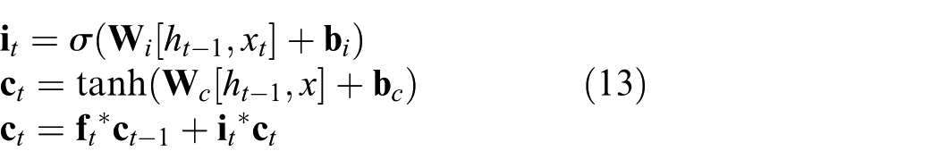
Output gate
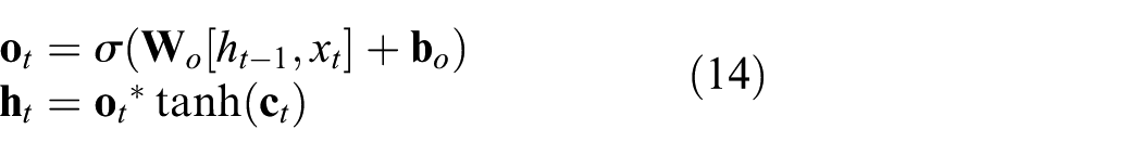
where

Structure of LSTM.
The proposed RUL prediction method
In this section, all steps of the proposed RUL prediction method will be explained in detail. We first provide the whole sketch map of the proposed method, as shown in Figure 4. Specifically, this method includes four parts: calculating HHT marginal spectrum data, health state assessment using the proposed SVD normalized correlation coefficient, deep feature extraction, and RUL prediction by LSTM regression. The detailed description of each part is given as follows.

Sketch map of the proposed RUL prediction method.
Calculating HHT marginal spectrum data
For the vibration signals used for bearing RUL prediction, time–frequency analysis is commonly used to evaluate the state change of bearing through the frequency spectrum. Since the instantaneous frequency of the HHT is defined as a function of time, 27 the HHT marginal spectrum is able to reflect the local characteristics of the signal more accurately. Unlike FFT, which needs a complete oscillation period to define the local frequency value, HHT is more suitable for non-stationary signal analysis. Since the vibration signal is non-stationary from normal state to degradation state, HHT is used to obtain the marginal spectrum as the input of deep learning model for feature extraction in this article.
Health state assessment
To divide the whole life of bearing into different health states accurately, a new criterion, named SVD normalized correlation coefficient, of health state assessment is proposed in this section. This criterion comes from the following idea: the correlation of singular value vector between normal state data is higher than the one between normal state and fault state data. With high numerical stability, the change of singular value will be small if slight perturbation of signal occurs. When the signals vary greatly, the singular value will change largely, which could avoid the negative effect of local noise and small perturbation for heath state assessment. Hence, the singular value can be used to precisely recognize state change when signals vary dramatically. Following this idea, we first divide the whole life of bearing into several sub-sequences. For each sub-sequence, phase space reconstruction is conducted by introducing Hankel matrix, whose singular value vector suits to represent bearing’s working state. 30 The steps of calculating this new criterion are as follows:
Phase space reconstruction for signal sub-sequence and calculation of singular value by means of SVD.
Suppose the raw signal is
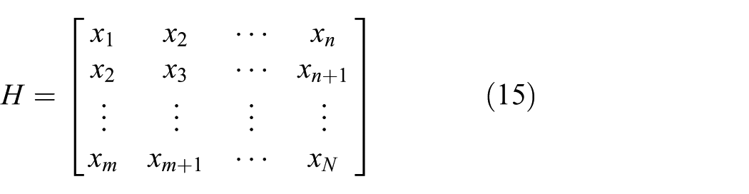
After SVD for

where
2. Normalization for the obtained singular value matrix.
The normalization can be conducted for singular value sequence using

where
3. Calculation of correlation coefficient for the normalized singular value matrix.
For the obtained normalized matrix, we choose the starting part of raw signal as the base value of normal state and then calculated the correlation coefficient with the singular value of each signal sub-sequence using

where
Deep learning feature representation
In order to predict the available remaining life, the effective feature representation of several heath states is required. As proven by many pioneer works in previous studies,14–18 deep learning techniques are good at extracting discriminative features directly from raw data. Therefore, we plan to exploit proper feature representation for two different health states: normal state and fast degradation. Specifically speaking, we set labels on these two states, and train classification model using one kind of deep learning algorithm, that is, CNN. In this process, deep features are adaptively extracted from frequency spectra through multiple-layer neural network, and a final classification is made through fully connected layer. The good classification performance will certainly indicate that the obtained deep features can effectively distinguish two health states and have good representation ability. Consequently, these deep features can be further used to construct RUL prediction model by means of temporal information.
It is worth noting that the input of CNN is the HHT marginal spectrum data, and the output is the classification label of two states, that is, normal state and fast degradation, which are automatically assessed using the proposed new criterion in section “Health state assessment.”
RUL prediction by LSTM regression
With the obtained deep features in section “Deep learning feature representation,” we need to build the RUL prediction model which should make full use of temporal information hidden in features. LSTM 23 network is an artificial network for temporal information modeling. With memory structure units, LSTM can select valuable short-term and long-term information and then save them, which is the difference between LSTM and most traditional time series prediction methods. Since the change amplitude of the vibration signal during the bearing degeneration process is rising gradually, this monotonous trend is exactly a kind of temporal information. Therefore, LSTM can be considered as an effective approach for RUL prediction with better performance than common regression models.
In the end, using the deep feature as an input and the corresponding RUL value as output, the LSTM model is trained for bearing RUL prediction. Please note that, as the signal trend of normal state does not change largely, RUL prediction is generally considered to be meaningful only since early fault of bearing occurred. Therefore, this article adopts the data in fast degradation state for RUL prediction. To determine the definite RUL value, a termination threshold of signal vibration amplitude should be fixed in advance. The formula of RUL calculation is
The threshold is generally suggested to set 20g, whose corresponding root mean square (RMS) value is 4.47. However, in some real-world data sets, the sampling of bearings has ended before their vibration amplitude reaching 20g due to some reasons. As a result, if we directly use the sampling end to calculate RUL value, the termination status for different bearings could not keep in same line, which will lead to inaccurate RUL value and then cause much bias of prediction result. Therefore, in this article, we first fit the available samples and second predict the following RMS trend. Then, the new RUL value can be obtained when the predicted RMS curve reaching the pre-fixed threshold. This process is illustrated in Figure 5.

Sketch map of RUL calculation using RMS curve fitting.
Specifically, in this article, we choose polynomial fitting to determine the new RUL value for the bearing data which do not reach the termination status. It is worth noting that the fitting order should be set 2 or 3. That is because the RMS curve in degradation process is monotonically increasing in general, but the fitting curve with order more than 3 will have no regularity and thus is unable to reflect the real degradation trend.
Once the RUL value and deep features are all determined, the regression model of RUL prediction can be built using LSTM. The flowchart of the proposed method is shown in Figure 6. To be specific, the input of LSTM is the extracted deep features and the output is the corresponding RUL value. Different from other traditional regression algorithms like SVM, this LSTM model can not only present the relationship between features and RUL value but also exploit the temporal information hidden in deep features at sequential time points in whole degradation process.

Flowchart of the proposed method.
Experimental results
In this section, computer experiments on one commonly used data set, the bearing data of IEEE PHM Challenge 2012, to verify the effectiveness of the proposed method are given. As the proposed method mainly includes deep feature extraction and LSTM prediction, we compare it with the traditional heterogeneous features and some regression algorithms. Each of the input variables is rescaled linearly to the range [−1, +1]. And, for Gaussian process regression (GPR) and SVM, the Gaussian radial basis function (RBF) kernel is used and defined as
Data description
The data set used in this experiment comes from the open IEEE PHM Challenge 2012. 20 This data set is collected from the test platform named PRONOSTIA, which can provide the whole run-to-failure vibration signal by conducting accelerated degradation experiment, as shown in Figure 7.

PRONOSTIA data collection platform.
PRONOSTIA consists of three parts: a rotating part, a degradation generation part, and a measurement part. The power of the rotating part’s motor equals to 250 W, which transmits the rotating motion to the test bearing. The loading part provides radial force for the test bearing to reduce bearing’s life duration. And, the measurement part is composed of two accelerometers which are placed on each bearing to pick up the horizontal and vertical vibration signals.
This prognostic challenge provides three groups of data under different operating conditions. In this article, we use the first group data with seven bearings which have the speed of 1800 r/min and load of 4000 N. We choose the horizontal signals for test because they can provide better results for tracking the bearing degradation. 5 The original test was stopped if the amplitude of the vibration signal overpassed 20g. But some bearings’ amplitude does not reach 20g strictly, which will bring inconsistent stop threshold. As a result, we need to determine the final RUL value for these bearings through unifying the stop threshold.
Experimental setting
Signal pre-processing
As discussed in section “Calculating HHT marginal spectrum data,” HHT is utilized to pre-process the raw vibration signal. Figure 8 shows the raw time signal of the bearing 1 under the first working condition and two kinds of spectrum in normal state, slow degradation state, and fast degradation state, respectively. By comparing Figure 8(b) and (c), FFT spectrum includes more noise than HHT marginal spectrum. Especially at high frequency of fast degradation state, HHT marginal spectrum changes more smoothly than FFT. Therefore, HHT marginal spectrum is considered to be more applicable for describing the degradation process of bearing than FFT spectrum.

The (a) raw signal, (b) FFT spectrum, (c) HHT marginal spectrum of the bearing 1 from IEEE PHM Challenge 2012 data set. Please note that the first row to the third row mean normal state, slow degradation state, and fast degradation, respectively.
Health state assessment
To determine the start point of fast degradation state and specify the state label for the extracted deep features, the proposed criterion which is mentioned above is used to assess the heath state for the bearing 1 in the first working condition. The results are shown in Figure 9, in which the blue curve is the smoothed RMS curve of bearing 1 and the red curve is the obtained correlation coefficient. It is obvious that the red curve keeps smooth and steady when the bearing works in normal state. But once the RMS rises dramatically, the coefficient curve falls down accordingly.

Health state assessment result using the proposed criterion for the bearing 1.
To determine a suitable threshold value, the following steps of calculating this criterion are adopted:
Calculate the RMS and SVD correlation coefficient of all seven bearings.
Take the maximum slope point of correlation coefficient as the base and then determine the corresponding change points on RMS curve, just like Figure 9.
Calculate the mean value of all seven bearings’ change points as the threshold value.
It is worth noting that the determination of threshold value will be more reasonable if more bearing data are available. In this article, the point with the value of correlation coefficient less than 0.95 is considered as the start point of fast degradation state. For better demonstration, Figure 10 shows the health state assessment results of other three bearings using this threshold.

Health state assessment of (a) the bearing 1, (b) the bearing 2, and (c) the bearing 7.
Similar to Figure 9, we use the proposed criterion to assess the heath state for all seven bearings under the first working condition. The results are shown in Figure 11. It is clear that the proposed criterion can determine the start point of fast degradation state for all bearings. Especially, the burr in the middle life of the bearing 6 does not disturb the assessment result, which demonstrates the effectiveness of the proposed criterion.

Results of heath state assessment using the proposed criterion. Here, the curves above the horizontal axis are the bearings’ RMS curve, and the ones under axis are the assessment results.
Deep feature extraction
Set the assessment results of the bearings 1–7 as class label, that is, normal state versus fast degradation state, and use the HHT marginal spectrum data of these two states as input, then train CNN to establish the deep model for feature extraction. Different from the traditional deep learning techniques, here, we introduce the class label in feature extraction. The reason is we want the extracted feature to express enough targeted information for degradation process.
Figure 12 provides the architecture of the used CNN network in this experiment. Specifically, the convolutional kernel of two convolutional layers both have the size 2 × 2, while these two layers’ feature maps are 64 and 128, respectively. The neuron number of full-connected layer is set 25, that is, the final feature dimension is 25. And, Softmax is used in the final layer for classification. 70% of the whole data are randomly selected for training and the remaining data are for test. Finally, we have the training accuracy 100% and test accuracy 99.52%.

Architecture of the used CNN network.
After training the deep model, we input again all data of the bearings 1–7 into this model to get the deep features. These features, extracted from fully connected layer, will be used for RUL prediction. To observe the feature distribution, we first apply PCA for the extracted deep features and then depict the distribution of the first three principal dimensions. Due to space limitation, we only take the bearings 1 and 7 for example, as shown in Figure 13.

Scatter plot of PCA components from CNN deep features on the data of (a) bearing 1 and (b) bearing 7. Here, the green points and red points mean samples in normal state and fast degradation state, respectively.
From Figure 13, we find that the green points and red points locate separately, which indicates the extracted deep features have obvious separability for normal state and fast degradation state. The results also testify the effectiveness of the deep features extracted from CNN model which has been trained in advance for classification task. High classification accuracy will lead to effective CNN deep features with good representation ability for two different states. Consequently, we think these deep features are applicable to characterize bearing’s degradation process.
It is worth noting that CNN can also perform as RUL prediction model through introducing actual RUL value as output information. However, there are many model parameters of CNN whose adjustment in training process is complicated and time-consuming. Although CNN is also able to get satisfactory prediction results, it is a big burden to determine model structure as it needs to represent the deep feature and learn nonlinear relationships simultaneously. For instance, we need to determine the size of filter, convolution layers, and pooling layers. Different from direct regression by CNN, this article merely uses CNN for feature extraction and then introduces temporal information rather than discriminative information of bearings’ degradation process for regression modeling. Although RUL value contains valid degradation information, these information need to be further exploited to find structural relationship, which is key to build a regressor. Therefore, we think temporal dependency between different time points will play a key role in RUL prediction. And, from the modeling perspective, the prediction model will be simplified by this way. LSTM is a kind of RNN with memory structure units, and it is professional to exploit the temporal dependency. And, according to our experience, the parameter selection and tuning of the proposed method using LSTM is exactly simpler than CNN with very similar prediction performance. Therefore, LSTM is used as the RUL prediction model in this article.
Determination of RUL value
We notice that for the all seven bearings under the first working condition in IEEE PHM Challenge 2012 data set, there are totally four bearings which do not reach the stop threshold of 20g. As discussed in section “RUL prediction by LSTM regression”, we need to evaluate the final RUL value for these bearings using the unified threshold of 20g. In this experiment, we utilize the polynomial fitting to fit the samples of these bearing and then predict the following degradation process. Specifically speaking, we first fit the degradation trend of the bearings 2, 5, 6, and 7, as shown in Figure 14. Here, the polynomial fitting with order 3 is applied for Figure 14(a), (c) and (d), while the fitting with order 2 is applied for Figure 14(b).
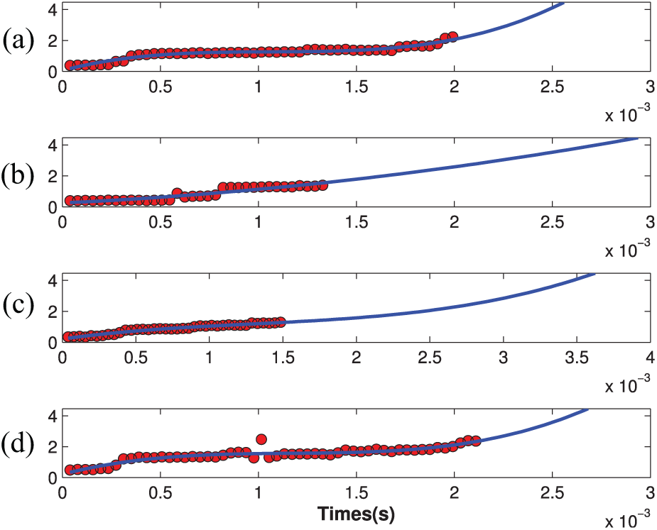
Determination of RUL using polynomial fitting for (a) the bearing 2, (b) the bearing 5, (c) the bearing 6, and (d) the bearing 7.
From Figure 14, the final RUL value can be calculated when the blue curve is reaching the stop threshold of 20g. We set the extracted deep features as the input and the final RUL value as output, then apply LSTM to establish the RUL prediction model.
Experimental results
Considering the limited sample size, we choose in order one bearing under the first working condition as the target one, while use the other six bearings for training. Finally, we use the prediction results on these seven bearings to evaluate the performance of the proposed method. Root mean squared error (RMSE) and mean absolute percentage error (MAPE) are introduced to evaluate the prediction performance with the following formula

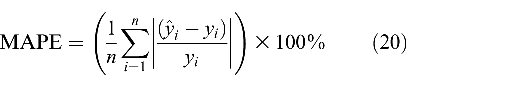
where
For comprehensive comparison, we set two kinds of experiments:
First, to evaluate the representation ability of the extracted deep features, we introduce 25-dimensional traditional statistical features in time domain and frequency domain. To test the comparative results, we run LSTM on the deep features and the traditional features. The definition of 25-dimensional statistical features is listed in Table 1.
Second, to evaluate the modeling performance of LSTM for temporal data, we introduce four traditional regression methods for comparison: linear regression (LR),
31
GPR,
32
SVM,
5
and extreme learning machine (ELM).
33
These four methods also use the same deep features extracted in section “Deep feature extraction” to train the regression model and then conduct RUL prediction for the bearing data in fast degradation state. These four methods all run model selection to determine the optimal hyper-parameters. For SVM, grid search and cross-validation are conducted to select the best kernel parameter
Definition of 25-dimensional statistical feature.

RMS: root mean square.
For the first kind of experiment, we run LSTM to conduct RUL prediction based on the deep features extracted by CNN and the traditional 25-dimensional statistical features. We take the bearings 1, 2, 5, and 7 under the first working condition as examples, as shown in Figures 15–18.
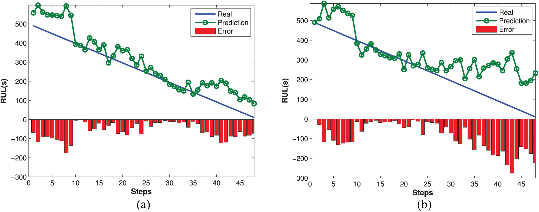
Results of RUL prediction using LSTM for the bearing 1 by means of (a) CNN deep feature and (b) 25-dimensional statistical feature.

Results of RUL prediction using LSTM for the bearing 2 by means of (a) CNN deep feature and (b) 25-dimensional statistical feature.

Results of RUL prediction using LSTM for the bearing 5 by means of (a) CNN deep feature and (b) 25-dimensional statistical feature.

Results of RUL prediction using LSTM for the bearing 7 by means of (a) CNN deep feature and (b) 25-dimensional statistical feature.
In each figure, the histogram under horizontal axis means the absolute error at each time point. From Figures 15–18, we find that the prediction curves using deep feature on all four bearings are closer to the real time line than the traditional statistical features, while deep features have smaller histogram error as a whole. These comparative results demonstrate that CNN can extract more discriminative and complete features for degradation process.
For the second kind of experiment, we mainly compare the prediction performance of LSTM and four traditional regression methods. Please note that, different from other four methods, LSTM has time memory units and is able to tackle temporal information. Due to space limitation, here we only compare the mean RMSE of all seven bearings. Because ELM and LSTM both adopt randomly initialized neurons, the randomness of prediction results is inevitable, even if it will decrease with the sample size increasing. To eliminate the negative effect of randomness, we repeatedly run 40 times of each method which has conducted model selection and calculate the mean value. The comparative results are shown in Figure 19. Besides, we also introduce the other two widely used deep learning algorithms, DSAE 18 and DBN, 19 to generate deep features. For DSAE, the noise level is set 0.01, the iteration number is set 100, and four hidden layers are adopted with size of [2048, 512, 128, 25]. For DBN, two restricted Boltzmann machines (RBMs) are adopted with the hidden neurons 2048 and 25. The iteration number of RBM and DBN are set 5 and 20, respectively. The learning ratio of RBM and DBN are both set 0.1. Please note that, to make an unbiased comparison, we set the dimension of deep features of CNN, DSAE, and DBN as 25.
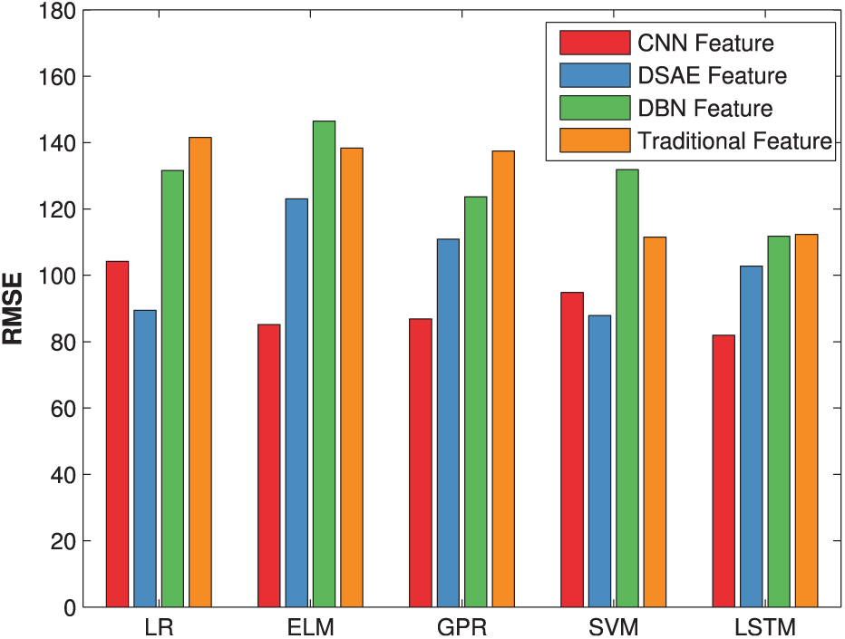
Comparative RMSE of five regression methods based on three kinds of deep features and traditional statistical feature.
From Figure 19, it is clear that LSTM gets lower RMSE than other four regression methods based on CNN deep features, which demonstrates the effectiveness of the proposed method. We also observe that with DSAE deep features, LR, and SVM get lower RMSE than LSTM. Actually, in our experiment, the prediction performance of LSTM varies to some extent in repeated trial. The fundamental reason is limited bearing data. In our experiment, we choose six bearings for offline training and the other one for online test. Although these seven bearings have same size, they still have different degradation trends. And, for each degradation process, the data are limited. As a result, LSTM has inevitable randomness when initializing network weights, which leads to the variation of prediction performance. In addition, we also notice that for five regression methods, CNN and DSAE both get lower RMSE than the traditional 25-dimensional statistical features, which further verifies the fault representation ability of deep features.
To further analyze the randomness of LSTM, we calculate the mean MAPE of 40 repeated trials for seven bearings. The comparative MAPE results are shown in Figure 20.
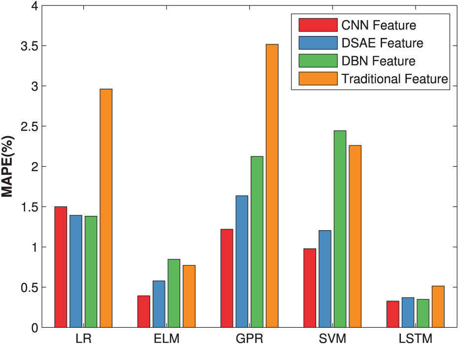
Comparative MAPE of five regression methods based on three kinds of deep features and traditional statistical feature.
From Figure 20, for LR, ELM, and GPR, the prediction error using deep features is generally lower than the traditional statistical features as a whole. And, for all five regression methods, CNN deep features are always better than the traditional statistical feature. Moreover, from the perspective of regression, LSTM has much lower prediction MAPE than other four regression methods. These comparative results further show the effectiveness of the proposed method for RUL prediction.
We also notice an interesting phenomenon. As the results of Figures 19 and 20 come from a same experiment, the RMSE of LSTM using CNN feature is higher than LR and SVM in Figure 19. However, in Figure 20, the MAPE of LSTM using CNN feature is instead much lower than the other four regression methods. That is because MAPE is a kind of relative error index. In the beginning of prediction, the data scale is obviously larger than the middle- to late-stage. As a result, small disturbance in the beginning would cause large variation of performance in terms of RMSE, even if MAPE has no obvious change. Therefore, we think MAPE is more applicable to measure the whole performance of RUL prediction.
Now, we provide the running time of the proposed method. Compared with the common machine learning models, the deep neural network is complicated while the training speed is relatively slow. Due to this reason, the process of deep feature extraction costs a long time, generally more than 30 s. And, for the regression model construction, the training time of LR, ELM, GPR, and LibSVM are 0.218, 1.37, 1.87, and 9.97 s, respectively. Also due to the deep structure, the training time of LSTM is 20.9 s, which is much longer than other regression models. Although this comparison looks huge, the training time of LSTM is still acceptable as it is merely for offline training. For online prediction, the test time is quite little to be zero. Therefore, we can claim that the proposed method is able to be applied to RUL prediction.
Besides the prediction error, we also evaluate the numerical stability of the proposed method. For Figure 20, we calculate the standard deviation of 40 trials, as shown in Table 2.
Standard deviation of 40 prediction errors in terms of MAPE.

MAPE: mean absolute percentage error; LR: linear regression; ELM: extreme learning machine; GPR: Gaussian process regression; SVM: support vector machine; LSTM: long short-term memory; DBN: deep belief network; DSAE: deep stacked auto encoder; CNN: convolutional neural network.
It is clear from Table 2 that the proposed method gets the standard deviation of 0.28. Although this value is not smallest, it is still much lower than the traditional statistical feature. Moreover, considering LSTM with CNN feature has lowest prediction result in terms of MAPE, we think this value of standard deviation can prove the numerical stability of the proposed method. Furthermore, nevertheless DBN gets lowest standard deviation, its MAPE is much larger than CNN and DSAE using ELM, GPR, and SVM. Even for LSTM, DBN’s MAPE is still larger than CNN. Consequently, we can say the proposed method using LSTM and CNN deep features has best comprehensive performance.
Conclusion
In this article, a new RUL prediction method based on deep feature and LSTM is proposed. This method integrates well the deep feature extraction for bearing degradation process and temporal regression using LSTM. The main idea of this method is using good feature representation ability of deep learning and regression ability of LSTM for temporal information to reduce the RUL prediction error and improve the numerical stability as well. From the experimental results, the following conclusions can be drawn:
Compared with the traditional statistical feature, deep feature extracted from CNN has better representation ability for bearing degradation process and thus can improve the RUL prediction performance.
Compared with the traditional regression methods, LSTM can make use of the temporal information of degradation process. With same features, LSTM can get lower prediction error and better numerical stability than other methods.
Compared with other deep learning algorithms, the proposed method has best comprehensive RUL prediction results in terms of MAPE and standard deviation.
In our next work, we plan to study the method of targeted deep feature extraction for RUL prediction. Ideally speaking, if we can give more instruction (e.g. the regression loss) for the unsupervised feature extraction process, the deep neural network can converge to a definite objective which can be more helpful to predict RUL. Moreover, structural information can also be introduced to deep learning techniques to improve the accuracy and stability of RUL prediction.
Footnotes
Handling Editor: Zhaojun Li
Declaration of conflicting interests
The author(s) declared no potential conflicts of interest with respect to the research, authorship, and/or publication of this article.
Funding
The author(s) disclosed receipt of the following financial support for the research, authorship, and/or publication of this article: This work was supported by the National Natural Science Foundation of China (Nos U1704158 and 11702087), China Postdoctoral Science Foundation Special Support (No. 2016T90944), the Funding Scheme of University Science & Technology Innovation in Henan Province (No. 15HASTIT022), and the foundation of Henan Normal University for Excellent Young Teachers (No. 14YQ007).