
Abstract
Engine as the core component of mechanical equipment, its operating state directly affects whether the equipment can operate normally. Predicting the engine remaining useful life (RUL) can monitor the health of the engine in real time and formulate a timely and reasonable maintenance plan. Aiming at the engine monitoring data with various and long time span, we propose a direct prediction method of engine RUL based on particle swarm optimization (PSO) optimized multi-layer Long Short-Term Memory (LSTM) in this paper. Firstly, the monitoring data that can well reflect the engine degradation trend is screened out, and the samples are constructed through a sliding time window. Then, a multi-layer LSTM model is constructed to mine the deep-seated features of the samples for predicting the engine RUL. Finally, the hyperparameters of the multi-layer LSTM model are optimized automatically by the PSO algorithm to optimize the performance of the model. The effectiveness of this method is verified by NASA data set. RMSE, MAE and the scoring function are used as evaluation indexes. RMSE and score of the prediction results are 12.35 and 284.1, respectively. It has higher prediction accuracy compared with traditional deep learning and machine learning methods.
Introduction
As the power source of mechanical equipment, the engine is one of the core components of the equipment. Its operating state and performance determine whether the equipment can operate stably and reliably. The engine operating conditions are complex and changeable, and the operating environment is relatively bad, resulting in a high failure rate of the engine. Once the engine failure occurs, it is easy to affect production and cause safety issues. Predicting the remaining useful life (RUL) of the engine can formulate a timely and reasonable maintenance and replacement plan to effectively solve problems existing in post-event or scheduled maintenance.
The RUL refers to the time that an equipment can operate normally after a period of normal operation. 1 Currently, there are three main types of RUL prediction modeling methods commonly used: model-based approaches, 2 data-driven approaches, 3 and based on hybrid model. 4 The model-based approaches need to establish a physical model according to the engine operating law and degradation process for prediction.5,6 As the structure of the engine becomes more and more complex and the fault characteristics are diverse. Establishing accurately a physical model is difficult. However, the data-driven approaches do not need to rely on a lot of engineering principles and professional knowledge, and predicts the RUL by mining the degradation laws directly from the collected engine monitoring data. With the development of computer computing power and the collection of a large number of sensor data, the data-driven approaches have become the mainstream.
Khelif et al. 7 used support vector regression (SVR) to establish a direct relation between health indicators and sensor values for RUL prediction, which reduced the steps of fitting equipment health status curve and establishing failure threshold. Shallow machine learning methods generally rely on expert experience and signal processing technology, extract features manually, and do not have an advantage in processing a large amount of historical monitoring data of equipment. Deep learning method has been widely used to process a large amount of monitoring data with its powerful nonlinear fitting and feature self-extraction capabilities and mining the potential features of the data as much as possible.8,9 Sbarufatti et al. 10 proposed the application of combination of sequential Monte-Carlo sampling and artificial neural networks (ANN) to the fatigue crack life prediction problem. Deutsch et al. 11 used Root Mean Square (RMS) to mine the signal features of sensor data and predicted the RUL of bearing through Restricted Boltzmann Machine (RBM). Babu et al. 12 proposed using one-dimensional convolution neural network (CNN) to process multi-dimensional sensor data to predict RUL. Ren et al. 13 proposed a method of bearing RUL prediction based on deep CNN. The eigenvector was extracted through the spectrum-principal-energy-vector. The monitoring data of equipment is generally multi-dimensional time series, and there is a correlation between before and after. The above prediction models do not take into account the time dependence of monitoring data. By introducing hidden state concept and memorizing key information, recurrent neural network (RNN) is able to efficaciously mine the time features in data. Long Short-Term Memory (LSTM) is superior in processing long-time sequence data by adding cell memory unit structure in hidden layer.14,15
Heimes 16 utilized RNN to predict the RUL of the equipment, and estimated directly the RUL through the model without feature extraction. Yuan et al. 17 applied three RNN variant models to predict RUL, and concluded that LSTM model had better performance by comparing the prediction results. According to the multi-dimensional monitoring information of the equipment, Malhotra et al. 18 utilized Encoder-Decoder based on LSTM to construct HI for the RUL prediction. There are two methods for data-driven RUL prediction: indirect prediction and direct prediction.19,20 Indirect prediction is according multi-dimensional sensor data to obtain one-dimensional HI curve, and performs RUL prediction based on the HI curve. However, direct prediction does not require obtaining the HI curve of sensor data, and directly extracts multi-dimensional fault features from multi-dimensional sensor data to predict RUL.
In this paper, we adopt a data-driven RUL direct prediction model, which maps the sensor data directly to the RUL of the engine. We propose a method to predict the engine RUL based on multi-layer LSTM network, and use the Particle Swarm Optimization (PSO) to adjust the hyperparameters of the multi-layer LSTM network automatically to improve the prediction accuracy.
The rest of this paper is organized as follows. Section II introduces the methods of data preprocessing and the basic theory of the RUL prediction method. Section III verifies the performance of the proposed method by turbofan engine degradation dataset. Conclusion is drawn in Section IV.
RUL prediction method
Multi-sensor data fusion method
The original sensor data collected from the sensor monitoring system consists of multivariate time series data from multiple sensors. Each engine corresponds to a number of data points obtained by sampling its multivariate sensor data over a period of time. The original sensor monitoring data of the engine is generally a multi-dimensional time series, and the sensor monitoring data of each engine is expressed as
We adopt the RUL direct prediction method based on the data-driven model.7,21 The collected sensor data maps to the engine health status directly. The RUL of the equipment system is predicted by performing pattern matching on multi-dimensional data and extracting m-dimensional fault characteristics that characterize degradation.
The collected engine sensor data includes a variety of variables, but not all sensor variables can characterize the failure process of the engine well. If the features are less correlated to the engine degradation characteristics, it will lead to insufficient fitting and affect the model training Effect. In order to screen out the variables whether can characterize or affect the engine operating state well and further compress the data to decrease the input dimension of deep learning model, this paper adapts the Pearson product-moment correlation coefficient to calculate the correlation among each variable. 22 Through correlation analysis, we select the valuable variables to determine the final variables used for model training.
The criteria for evaluating the correlation between sensor characteristics and time are defined as follows:
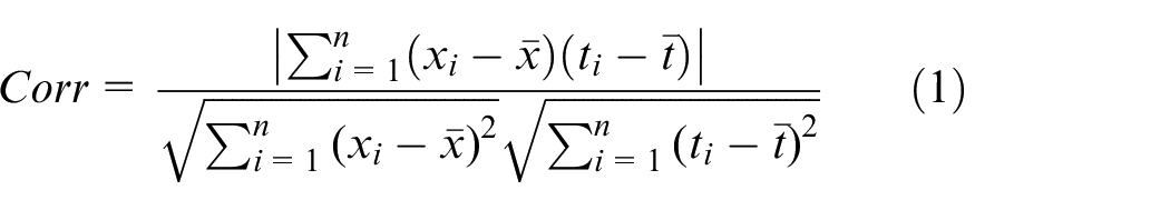
Where
The variables that characterize the engine failure process not only show high correlation, but also should have a monotonous trend.23,24 The monotonicity of variables indicates that the engine failure gradually increases until it fails. So the feature selection is realized by calculating the correlation and monotonicity between sensor data and engine degradation process. The collected sensor data will be affected by noise, so we use the improved monotonicity criterion to evaluate the monotonic trend performance of sensor features.
The monotonicity criteria for evaluating the monotonic trend performance of sensor characteristics are as follows:
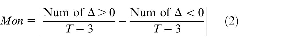
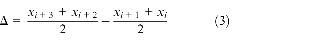
Where
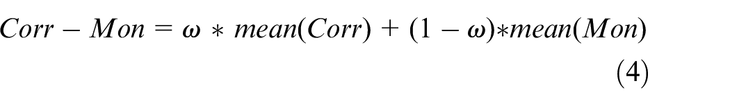
Finally, the sensor data is selected through the linear combination composite criterion (
Data preprocessing
Sensor data is inevitably affected by environmental noise and sensor errors during the collection and transmission process. In order to avoid the adverse impact of some wrong data on modeling, it is necessary to preprocess sensor data.
The different value ranges and units of the collected sensor variables lead to large numerical gaps, which will affect the training result of the deep learning model and reduce the prediction accuracy. Therefore, the data needs to be standardized to reduce the difference between the data. In this paper, z-score standardization is used to standardize collected sensor variables, so that the standard deviation of each sensor variable is 1, and the mean value is 0. The formula is as follows:
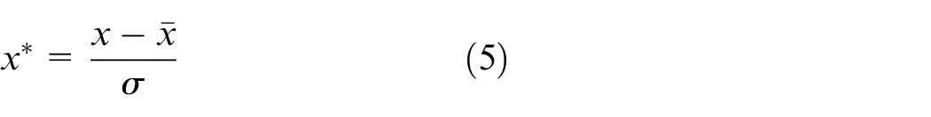
Where σ represents the original variables standard deviation,
In this paper, the sliding time window method is used to generate training samples to meet the input form of the LSTM model. The data input to the model each time is a two-dimensional tensor of size
Multi-layer LSTM model construction
The sensor data reflecting the engine degradation trend is time series data. RNN is a model specially for processing time series data, which includes input layer, output layer and hidden layer. The data of the current sequence is affected by the historical output data. The output of the current moment feeds back to itself and participates in the input of the next moment. LSTM is improved on the basis of RNN. The cell memory unit structure is added to the RNN hidden layer, which makes the model have the ability to learn long-term dependent information. 25 The problems of gradient explosion or gradient disappearance can be overcome effectively. And it is more advantageous than RNN in solving the problem of long-term data series.
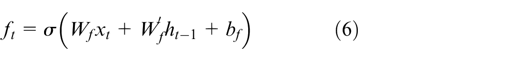
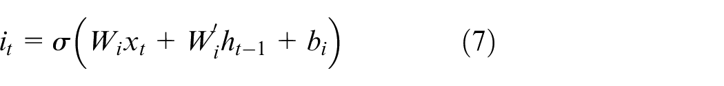
LSTM neural network introduces three gate structures in the hidden layer, including input gate, forget gate, and output gate, which are used to control the update and forgetting of memory to realize the storage and flow of memory in the hidden layer unit.26,27 The LSTM cell expanded by time series is shown in Figure 1.
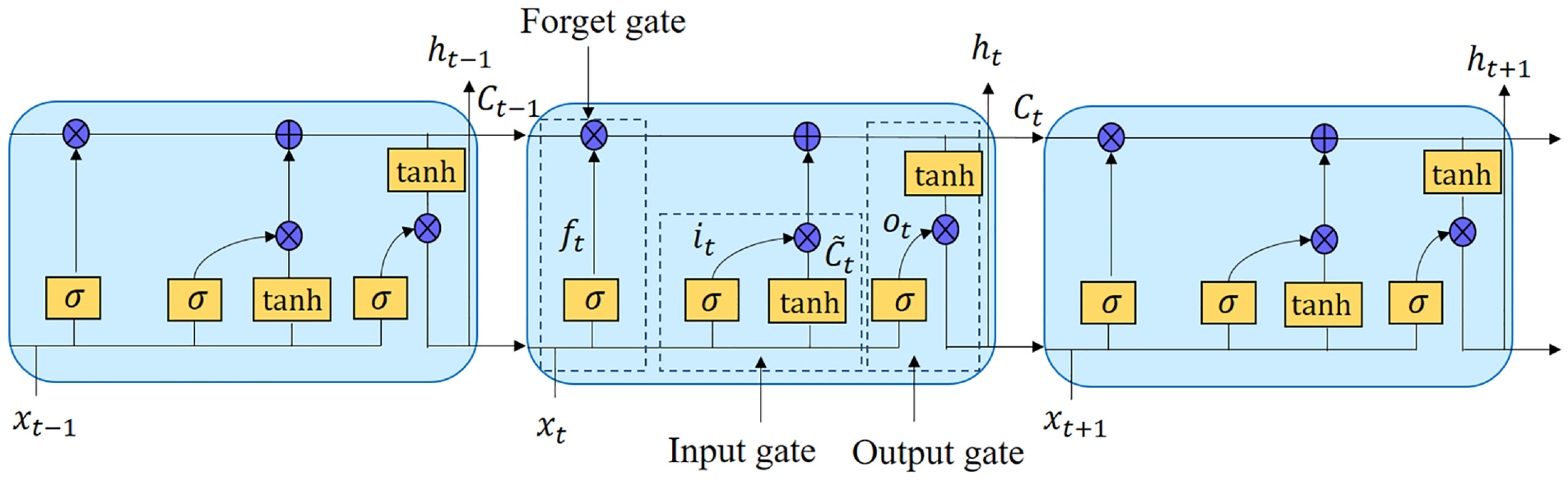
LSTM cells expanded in time series.
In Figure 1,

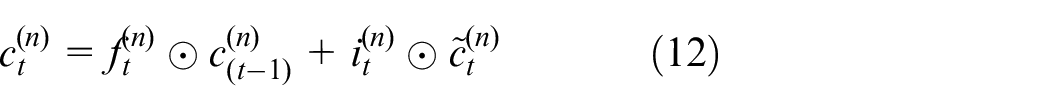
Update the cell state by modulating the previous cell state to the current cell state.

The cell state value and the result of the output gate determine the final output:
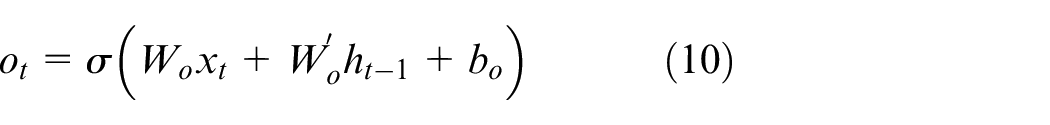

In the formula,
In this paper, the method of superimposing multi-layer LSTM is used to mine deep abstract features. Use the output of the previous layer of the model as the input of the latter layer to improve the non-linear fitting ability. The state of the nth layer at time

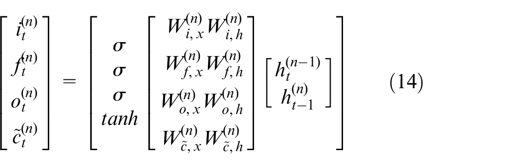
Where
Finally, the final prediction RUL of the engine is output by connecting the fully connected later behind the multi-layer LSTM. The final output is expressed as:

In the formula,
Particle Swarm optimization
The prediction accuracy of the model and the fitting degree of the results are affected by the hyperparameters of the multi-layer LSTM model such as the number of neurons in every LSTM layer, the time window size, and the batch size. Manual parameter adjustment is inefficient and not easy to find good parameters. Swarm intelligence optimization algorithm has strong global convergence and robustness, and does not depend on the strict mathematical properties of the optimization problem itself, so it can be used to optimize the hyperparameters of the network. The PSO has the advantages of simplicity, effectiveness, and easy implementation, and has great potential in optimizing neural network.
The PSO is a kind of stochastic optimization technology based on population, which imitates the swarm behavior of bird flocks. Each particle in the search space represents a solution. Suppose m particles forming a particle swarm fly in an n-dimensional space at a certain velocity. Each particle is composed of three n-dimensional vectors: the position vector


When the entire group is searching for a target, each particle often adjusts the next search through the optimal position it has reached and the optimal position searched by the entire group. In the iterative process, the fitness value of every particle is calculated, the velocity is updated and the direction is corrected. Lastly, the target optimal position is found, that is, the optimal result of the question. By sharing the information about the target position between groups, the velocity of finding the target can be accelerated. The particles update their own velocity and position according to the following two formulas 28 :
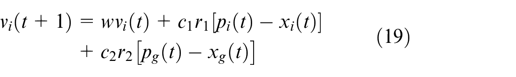

Where
Step 1: Take the hyperparameters of the multi-layer LSTM model to be optimized as the particles, and set the value range and the maximum velocity
Step 2: Initialize the population size, velocity, and position of the particles, each particle is composed of a multi-dimensional real number vector, and initialize
Step 3: Take the vector corresponding to each particle as the parameter value of the multi-layer LSTM model to form the network, and input the training sample data for training.
Step 4: Set the evaluation index such as score of the prediction result as the fitness value, obtain the fitness value of each particle, and determine
Step 5: Determine whether the algorithm meets the termination conditions. If the termination conditions of the algorithm are met, execute step 7, otherwise, execute step 6.
Step 6: Update the position and velocity of the every particle through the above (19) and (20), and go to step 3 for iteration.
Step 7: Obtain a set of global optimal values
General procedure of the proposed method
The overall process of the engine RUL prediction method based on PSO optimized multi-layer LSTM neural network is shown in Figure 2. It is mainly divided into the following steps:
Step 1: Data preprocessing.
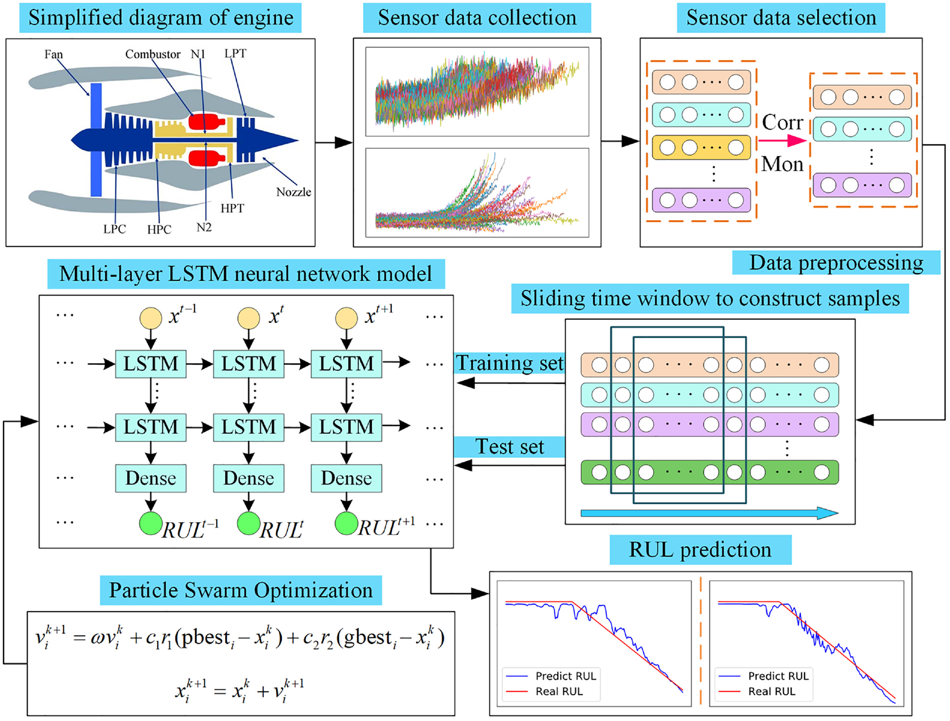
General process of the proposed method.
The training set is composed of the historical monitoring data of the engine, and the multi-dimensional engine data that can well reflect the engine degradation trend is screened out through the composite standard of correlation and monotonicity. Then, the screened out data is preprocessed through z-score standardization to eliminate the effect of the difference in units and value ranges between different indicators.
Step 2: Sliding time window to construct training samples.
The processed training data is used to construct training samples through a sliding time window to generate a two-dimensional tensor with a fixed time window size. And the RUL corresponding to the last time in the time window is taken as the sample label. If the monitoring data is smaller than the time window size, add zeros after the data to generate training samples.
Step 3: Constructing multi-layer LSTM model.
The RUL prediction model of engine based on multi-layer LSTM is constructed. The preprocessed training samples that conform to the input of LSTM model are input into the constructed model to train. And divide a part of the training set as the validation set to cross training.
Step 4: RUL prediction.
The test set of the engine monitoring data is preprocessed according to steps 1 and 2 to construct test samples and input them to the trained LSTM prediction model. Output the engine RUL value predicted corresponding to the last time of the time window.
Step 5: PSO optimization.
Optimizing automatically the hyperparameters such as time window size, the number of neurons in every LSTM layer, and the batch size of the multi-layer LSTM prediction model improves the degree of fitting, the model performance, and the prediction accuracy.
Step 6: Evaluation of the prediction method.
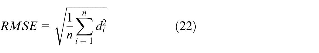
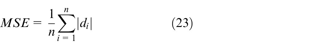
The predicted engine RUL is compared with the actual engine RUL, and the performance of the prediction model is evaluated by the scoring function (S), 29 RMSE, 30 and MAE. 31 The formulas are defined as follows:
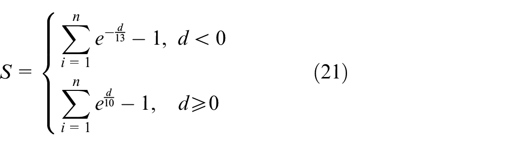
Where n represents the number of samples in the test set,
RUL prediction method
Engine experimental data
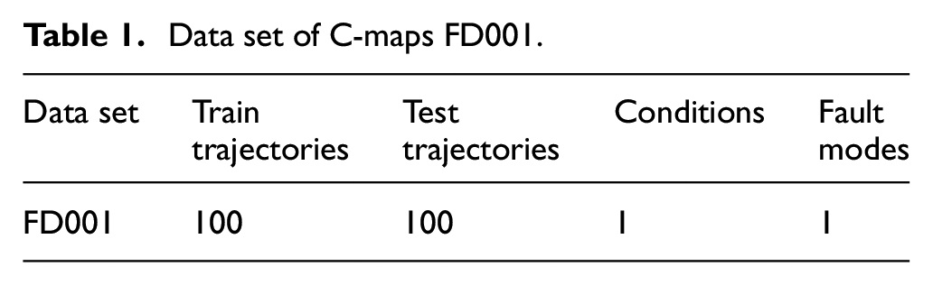
This paper uses the C-MAPSS data set 32 as experimental data to test the effectiveness of the proposed method. The data set is provided by NASA’s Prognostics Center of Excellence, and the turbofan engine is taken as the specific experimental object. Each sub data set includes both training set equipment and test set equipment. The Data set contains 26 columns of numbers and is composed of multiple multi-dimensional time series. There are 21 columns of sensor monitoring data, unit number, time, and three columns of operational settings. The turbofan engine in the training set has complete run-to-failure data with labels. The test set only provides the previous data in the whole life cycle, and the RUL is used as result validation in the RUL_FD00X document. In this paper, FD001 sub data set is mainly used as experimental data, including 100 training set data and 100 test set data listed in Table 1.
Data set of C-maps FD001.
The system performance of the turbofan engine is in a healthy condition at the beginning of operation. The turbofan engine starts gradually to degrade after a period of operation, and the degradation intensifies toward the end of its life. Therefore, a piece-wise linear RUL label is used to take the place of a simple linear RUL label. The maximum RUL of the turbofan engine is set as 120–130,33,34 so that the model can better extract the degradation features and improve the prediction accuracy.
Multi-sensor data fusion and filter
The FD001 training set and test set record three operational settings and 21 engine sensor data. To screen out the variables that can represent or greatly affect the engine state, the correlation and monotonicity of each parameter in the training set are calculated through correlation and monotonicity criteria. Divide the data of every 25 engines in the training set into a group, and the results of each group are averaged. The result is shown in Figure 3.
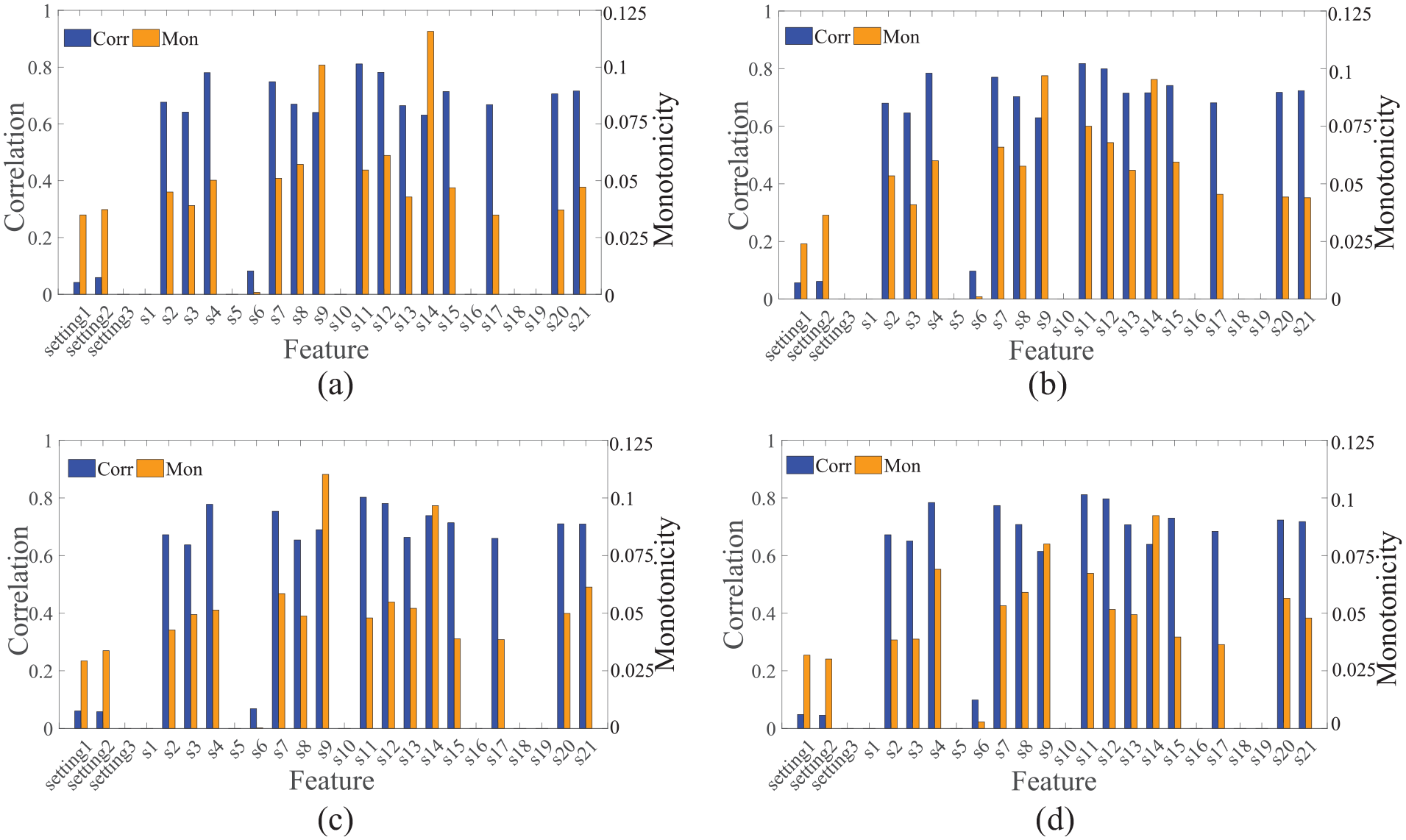
Correlation and monotonicity mean of FD001 data: (a) id: 1–25, (b) id: 26–50, (c) id: 51–75, and (d) id: 76–100.
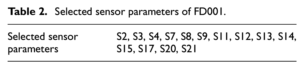
Then, the parameter characteristics that meet the threshold conditions are screened by compound criteria. This paper sets the threshold to 0.5. It can be seen from Figure 4 that the sensor parameters selected in each group are the same. The selected parameter characteristics are shown in Table 2.
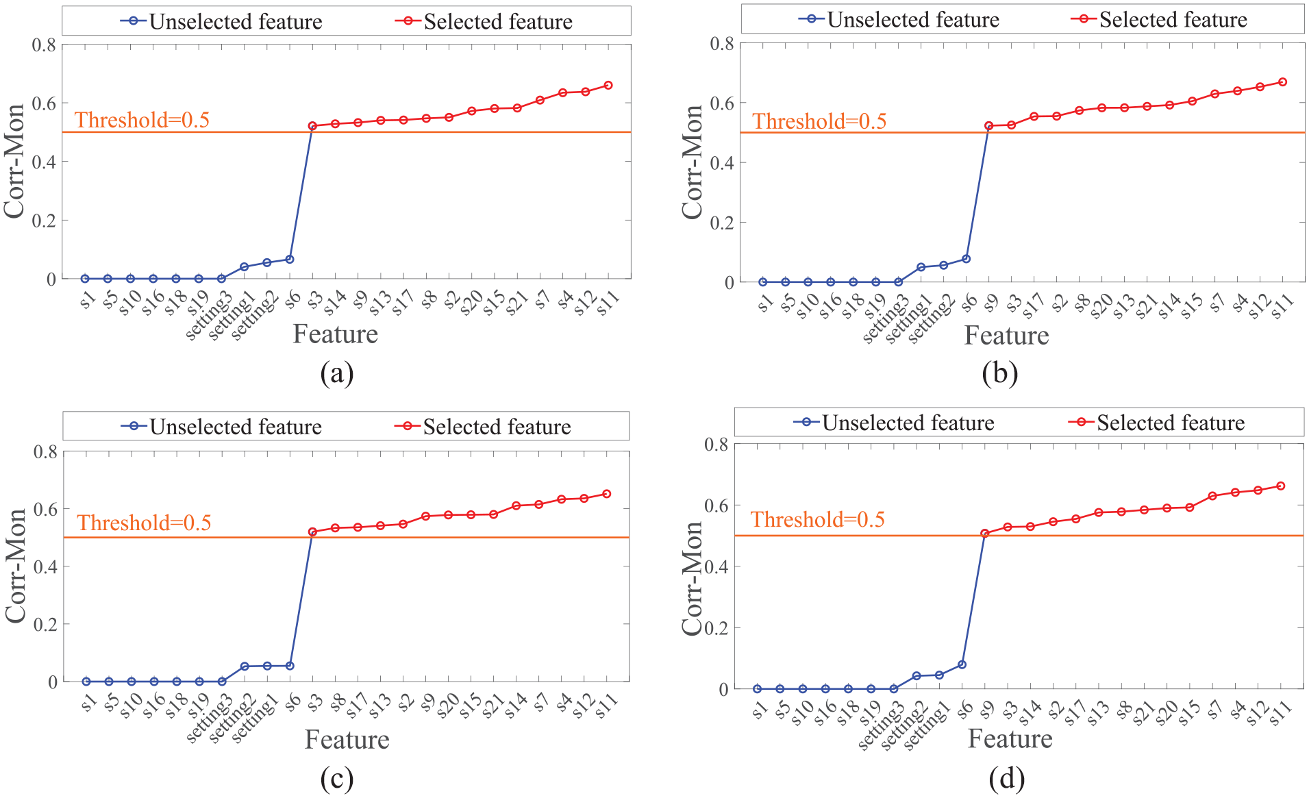
Corr-Mon compound criteria of FD001 data: (a) id: 1–25, (b) id: 26–50, (c) id: 51–75, and (d) id: 76–100.
Selected sensor parameters of FD001.
The selected parameter features are preprocessed by z-score standardization, and then training samples are constructed by sliding time windows, which are used as input for the subsequent models.
RUL prediction using multi-layer LSTM neural network
This paper adopts the prediction method of mapping engine monitoring data directly to RUL and takes the FD001 sub data set as the experimental sample. We input the processed training samples into the multi-layer LSTM neural network model for training and divide 10% of training samples from the training set into the validation set for cross-validation. The final output layer is the Dense layer of a neuron, whose activation function is ReLU, which outputs the predicted RUL of the engine. This model uses Adam optimization method for gradient optimization, 35 and the loss function used is the RMSE function. Finally, we input the processed engine test set data into the trained model to predict its RUL.
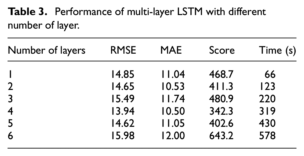
Compared with one layer LSTM, superimposing multi-layer LSTM can extract deeper sequence features, but too many layers of the LSTM network will also cause problems such as increased training time and overfitting. Therefore, the LSTM layer number comparison experiment from one layer to six layers was set up to explore the influence of different number of layers on model performance. The experiment of each layer number was run multiple times. The results are taken as the averaged and shown in Table 3. As shown in Figure 5, the prediction results are better when the number of layers is four or five, but the error increases significantly when the number of layers increases to six.
Performance of multi-layer LSTM with different number of layer.
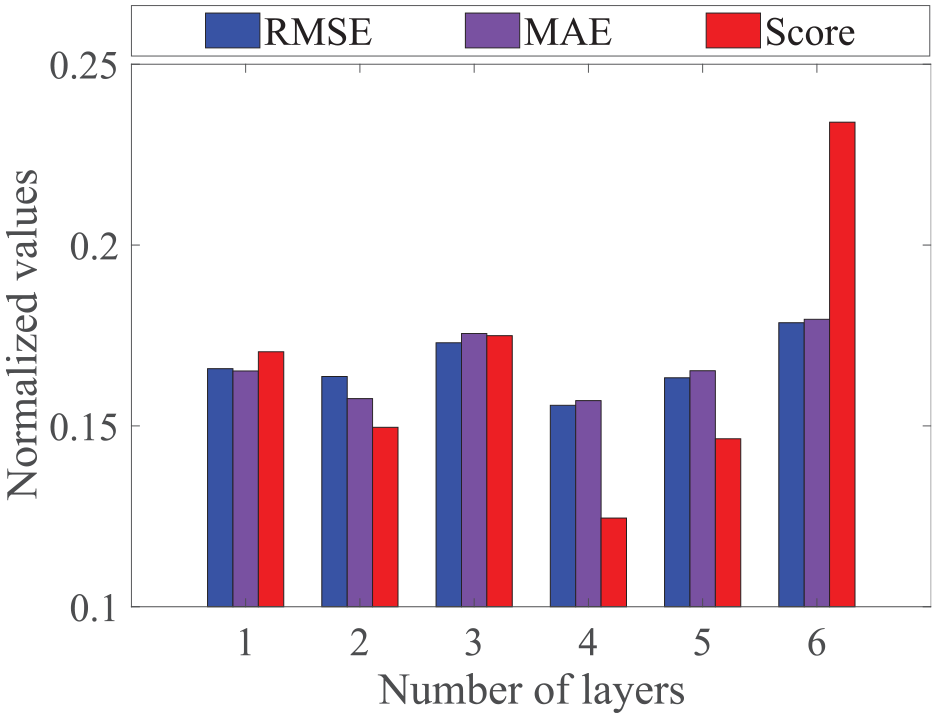
Normalized values of evaluation criteria for different number of layers.
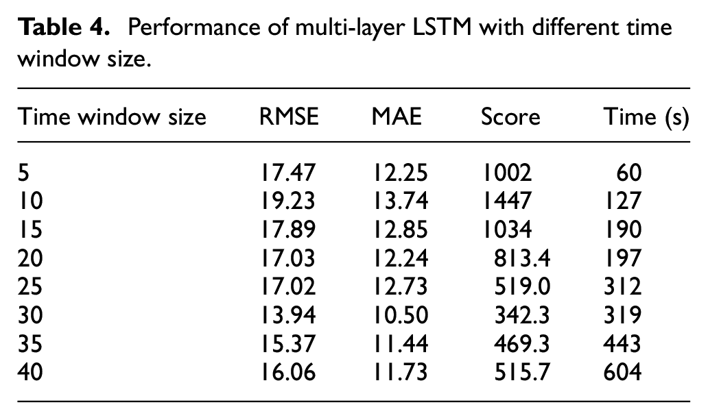
The next step is to choose the length of the time window. Choosing an appropriate size of the time window, the RUL of the engine can be well predicted. On the basis of the four-layer LSTM, eight groups of time window sizes of 5, 10, 15, 20, etc. were carried out to compare the influence of different time window size on the model performance. The results are shown in Table 4. We can see from Figure 6 that the prediction result is better when the time window size is about 30.
Performance of multi-layer LSTM with different time window size.
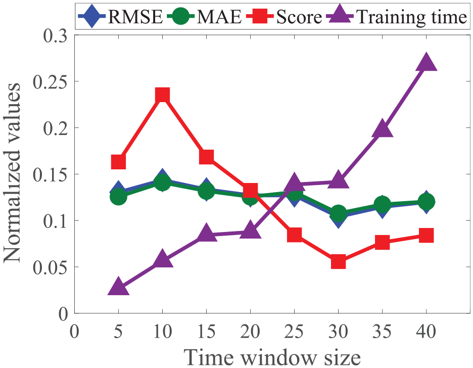
Normalized values of evaluation criteria and training time for different time window size.
According to the layer number experiment and time window size experiment, the time window size selected in this paper is 30, and the layer number of LSTM model is set to 4.
RUL prediction using PSO optimized multi-layer LSTM neural network
The number of neurons in every layer and the batch size of the multi-layer LSTM model also greatly impact the prediction accuracy of the model. Manual parameter adjustment is inefficient and it is difficult to find good parameters. The PSO algorithm has the superiority of high precision and easy implementation. The method of PSO automatic parameter adjustment is used to optimize the multi-layer LSTM neural network model to improve the prediction accuracy and performance of LSTM model.
On the basis of the four-layer LSTM and the time window size of 30, the number of every LSTM layer neurons and the batch size of the model are taken as the particles of the PSO algorithm. The value range of the number of every layer neurons is set to [10, 200], and the value range of batch size is set to [10, 520]. Set the scoring function evaluation index of the LSTM model prediction result as the fitness value. And set the group size m to 20 and the maximum velocity
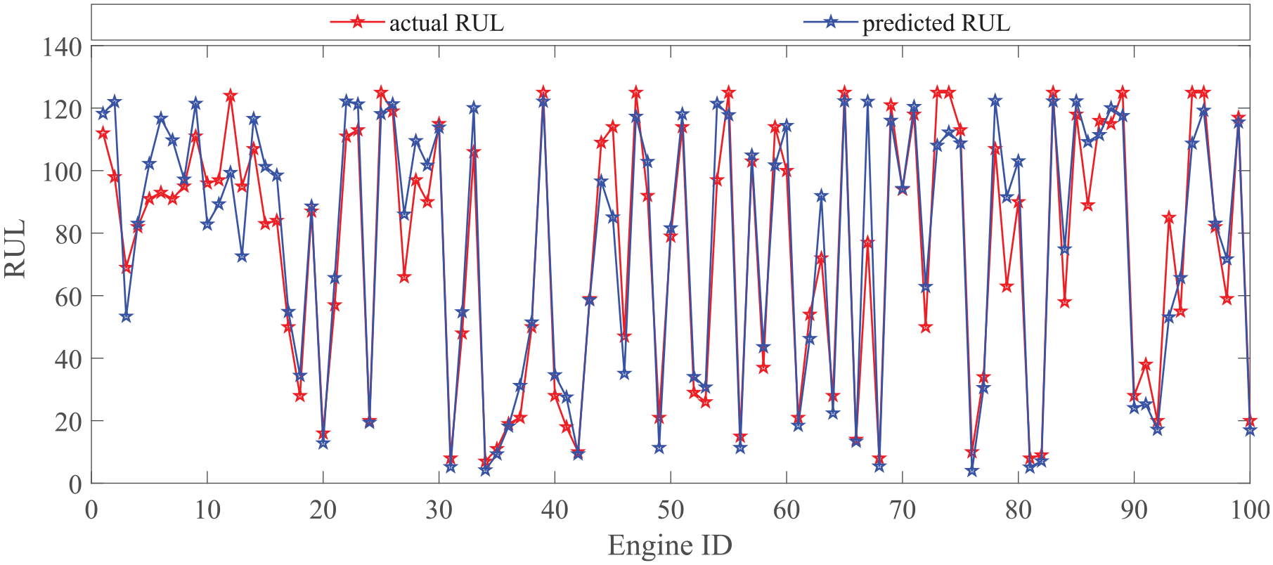
RUL prediction result of FD001 test data.
Comparison of the proposed method and traditional methods
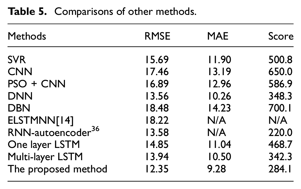
The multi-layer LSTM network model optimized based on PSO is compared with SVR, CNN, CNN + PSO, DNN, DBN, ELSTMNN[14], RNN-Autoencoder[36], basic LSTM, and multi-layer LSTM network model that is not optimized to test its performance. The CNN model has five layers in this paper, including two convolution layers (Conv1 and Conv2), two max-pooling layers (Maxpooling1 and Maxpooling2), and one fully connected layer (FC). In the CNN + PSO method, the number and size of convolution kernels are taken as hyperparameter to be optimized. The deep neural network (DNN) has four hidden layers. The number of neurons in the hidden layers is 500, 400, 300, and 100, respectively. The structural parameters (i.e. the number of hidden layers and the number of hidden neurons per hidden layer) of the deep belief network (DBN) strongly depend on problem complexity and the number of available training samples. Given the complexity of our studied problems and the limited number of available training samples, the number of hidden layers and the number of hidden neurons per hidden layer in a DBN are not set to be very large in our experiments. Specifically, the number of hidden layers for each DBN is set to three. We can see from the Table 5 that the prediction accuracy of the model optimized by the PSO algorithm has been greatly improved, with reductions of 11.4%, 11.6%, and 17% in the RMSE, MAE, and Score functions compared to before optimization. The prediction results of an engine in the test set of different methods are shown in Figure 8. Compared with other models, the predicted RUL of LSTM network model is closer to the real RUL in the degradation process, especially in the second half of the degradation process, the predicted RUL curve is smoother. The confidence interval of LSTM network model in the second half of the degradation process is also relatively small fluctuations, the general range is near the true RUL, indicating that the LSTM model can predict RUL well in the later stage of operation, and the stability and repeatability of the prediction results are better. Compared with the four-layer LSTM network model, the optimized model can fit the actual RUL better in the degradation process of the engine, and the fluctuation of the predicted value is smaller, and it can also fit the actual RUL better in the early stage of the degradation stage. We can see from the Table 5 and Figure 9 that LSTM model has advantages over other methods in processing long-time series problems. In the comparison of RMSE, MAE and score, the prediction results of the proposed method are the best.
Comparisons of other methods.
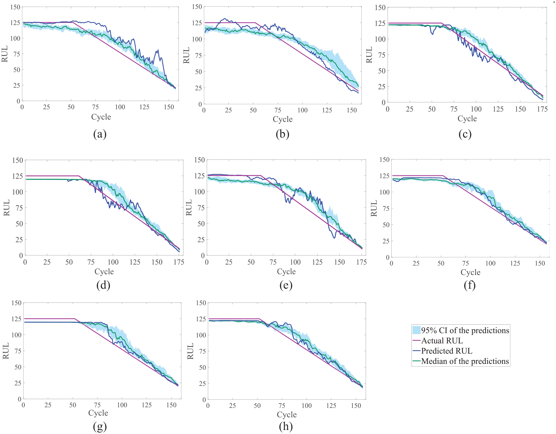
Partial results of RUL prediction with different methods: (a) SVR, (b) CNN, (c) PSO + CNN, (d) DNN, (e) DBN, (f) one layer LSTM, (g) multi-layer LSTM, and (h) the proposed method.
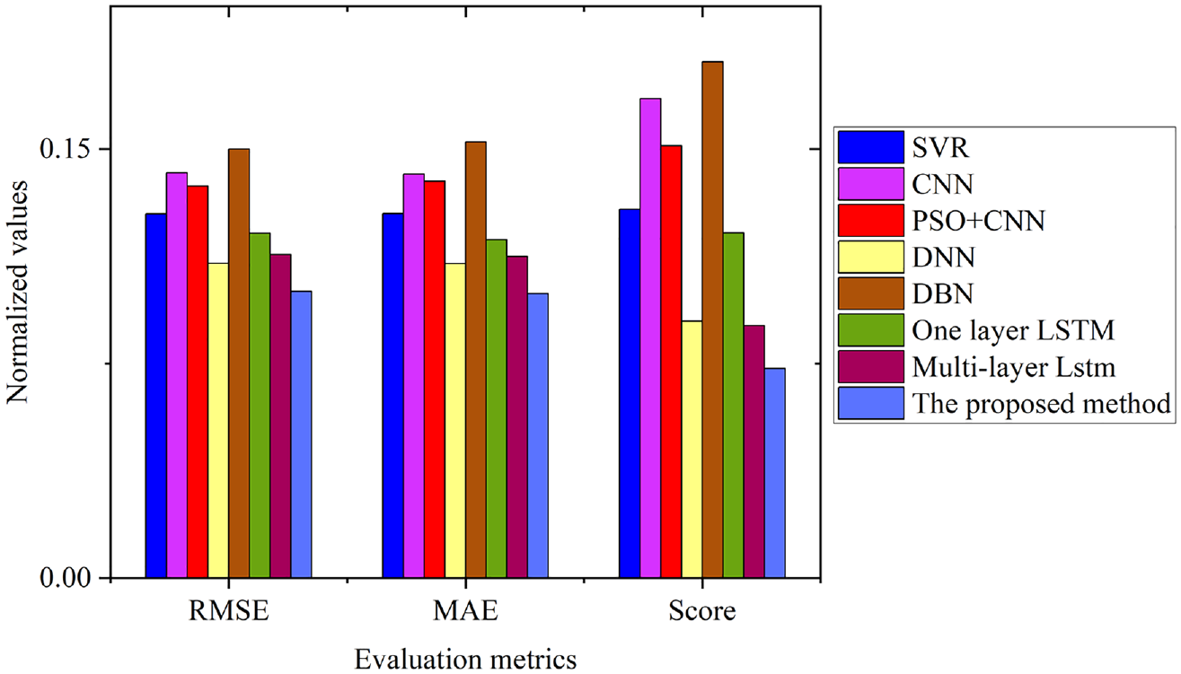
Normalized values of evaluation criteria for different methods.
Conclusions
This paper proposes a direct prediction method of engine RUL based on PSO optimized multi-layer LSTM neural network. Through the composite standard of correlation and monotonicity, the sensor monitoring data that can well reflect the engine degradation trend can be effectively screened out. By standardizing the data, the effect of units and value range between different sensor data is eliminated. The training samples are constructed by sliding time windows, and the correlation between the front and back of the sensor data sequence is preserved. Combined with the superiority of LSTM neural network in processing time series, the engine RUL prediction model of multi-layer LSTM is established to fully excavate the time characteristics of data and predict the RUL of engine. PSO algorithm is used for adjusting automatically the hyperparameters of the LSTM prediction model, optimize the performance of the model, and overcome the time-consuming and tedious shortcomings of manual parameter adjustment. Use NASA’s C-MPASS data set as experimental data to verify the performance of the proposed method. The comparison results show that this method has advantages over other methods in prediction accuracy.
Footnotes
Declaration of conflicting interests
The author(s) declared no potential conflicts of interest with respect to the research, authorship, and/or publication of this article.
Funding
The author(s) disclosed receipt of the following financial support for the research, authorship, and/or publication of this article: 2018YFE02013 and Grant 2020YFE0204900, and Key Research and Development Plan of Shandong Province under Grant 2019TSLH0301 and Grant 2019GHZ004.