Sage Journals: Discover world-class research

Abstract

It is difficult to develop accurate mathematical models to describe the range extender electric vehicles due to the non-linear and complex coupling of the monitoring signal sources resulted from the massive moving parts and complex architecture in range extender and the limited storage space of the diagnostic device. In this study, we proposed the smooth iterative online support tensor machine algorithm, which is combined with support higher-order tensor machine and online stochastic gradient descent method, and applied it to the fault diagnosis of the range indicator. Four methods with different algorithms, support vector machine, smooth iterative online support vector machine, linear support higher-order tensor machine, and smooth iterative online support tensor machine algorithms, were adopted to diagnose and classify the fault samples of the range indicator by comparing the diagnostic accuracy and model learning time. It is found that the fault diagnosis method based on the smooth iterative online tensor machine showed a higher accuracy, shorter learning time, and less storage space. Based on the experimental results, it is feasible to apply smooth iterative online support tensor machine model to the fault diagnosis of electric vehicle extenders.

Keywords

Electric vehicle range extender fault diagnosis smooth iterative online support tensor machine smooth iterative online support vector machine

Introduction

Due to the shortage of energy and environmental pollution, the development of traditional electric vehicles is restricted while the extended electric vehicles have been developing fast.¹ However, the fault of range extender will directly affect the reliability and safety of the electric vehicles. Therefore, to improve the safety, reliability, and economy of the extended range electric vehicles, it is of great significance to diagnose the working condition of range extender accurately.^2,3 For the extender-fault diagnosis technology, the traditional simple diagnosis method was first applied and then the conventional diagnostic technology based on sensor, dynamic testing, and signal processing was developed. With the improvement of the computational technology, intelligent diagnosis technology methods using artificial intelligence have been developed, which includes expert system fault diagnosis method,⁴ particle filter diagnosis method,⁵ multi-source information fusion diagnosis method,⁶ neural network diagnosis method,⁷ and support vector machine (SVM) diagnosis method.⁸

Traditional intelligent diagnosis techniques are using the vector as input samples for classification learning, which would easily result in the loss of information and destroy data correlation structure. To avoid these problems, Tao et al.⁹ proposed support tensor learning (STL), which extends the vector classification model to tensor patterns by making full use of the structural information of the data and their correlation. In 2013, Hao et al.¹⁰ proposed a support higher-order tensor machine (SHTM) model, which uses CP decomposition to reduce computational and storage space greatly. In 2015, Liu et al.¹¹ designed the concave-convex procedure-based transient support tensor machine (CCCP-TSTM), which can solve the nonconvex sample problems and shorten the iteration time. As the expansion and complement of the vector model, the tensor model has a certain improvement in the fault diagnosis accuracy and the sample learning time. In recent years, many researchers have put forward various learning algorithms based on tensor pattern, which has aroused wide attention and application, such as face recognition,^12,13 data mining,¹⁴ machine learning,¹⁵ computer vision,¹⁶ and three-dimensional liquid crystal flows.¹⁷

The above models often use batch or off-line learning methods. However, in the engineering application of extender failure prediction, the signal data for machine learning are collected one by one in a sequence and sent to the learning system in an endless stream. It is unrealistic to proceed the machine learning in favorable performance with one or several stationary classifiers for the long and changeable data sequence.¹⁸ In this case, the training for large-scale samples will not only cost a long time but also have a relatively low precision. Therefore, the online learning algorithm is introduced into the prediction model.¹⁹ The common online learning algorithms include online support vector classifiers (OSVC),²⁰ online independent support vector machine (OISVM),²¹ double updating online learning (DUOL),²² and adaptive and self-confident on-line learning.²³ Because of low cost, time consumption, and high precision of online learning for large-scale samples, online learning is applied to multiple fields, such as dynamic two categories,²⁴ vowel imitation learning,²⁵ and modular robots.²⁶

In this article, the smooth iterative online support tensor machine (SIOSTM) algorithm was developed by combining the two algorithms of linear SHTM and online stochastic gradient descent (OSGD). Using the tensor-type data as input, the characteristic parameters of the fault samples of the electric vehicle extension were extracted and the fault parameters were diagnosed.

SIOSTM

In pattern recognition, machine learning, computer vision, and image processing and other research areas, such as face image,²⁷ are represented by second-order tensor; color image,²⁸ gray video sequence,^29,30 silhouette sequence,³¹ and multispectral image³² are usually expressed as third-order tensor; color video sequence^33,34 can be seen as fourth-order tensor. The fault diagnosis samples in this article are represented as third-order tensor.

In this article, we propose the SIOSTM and take the fault samples of the third-order tensor as the classification object. In 2013, R Zhou et al.³⁵ proposed the online support tensor machine (OSTM), but with the algorithm for fault diagnosis, it was found that when the number of samples was small, the algorithm was difficult to obtain the optimal hyperplane. In addition, the Lagrange multiplier will oscillate in the process of online iterative updating, so that it is difficult to converge. To solve this problem, we propose SIOSTM. The Lagrangian multiplier in the initial iteration has been close to the optimal hyperplane, and in the process of online learning is a smooth iterative way to achieve the optimal value.

Smooth iterative online support vector machine

Using the basic formula of tensor and the definition of n-modulus and norm, the alternate projection algorithm proposed by Q Zhao et al.³⁶ is simplified as the SVM model with the tensor as the input sample, also known as the generalized support tensor model

min_{W, b, ξ} \frac{1}{2} ‖ W ‖_{F}^{2} + C \sum_{i = 1}^{l} ξ_{i}

(1)

s . t . y_{i} (〈 W, X_{i} 〉 + b) \geq 1 - ξ_{i}

(2)

ξ_{i} \geq 0, i = 1, 2, \dots, l

(3)

where the weight parameter $W$ and the input sample $X_{i}$ are same scale-sized tensor-type data.

Based on model (1)–(3), we have proposed online learning. Because we only can deal with one sample at a time by online learning, so select a sample ${X_{t}, y_{t}}$ arbitrarily, and $ξ_{t} = max (0, 1 - y_{t} (〈 W, X_{t} 〉 + b))$ , the following cost functions are considered

Q (W, b) = \frac{1}{2} ‖ W ‖_{F}^{2} + C max (0, 1 - y_{t} (〈 W, X_{t} 〉 + b))

(4)

Then

\frac{δ Q (W, b)}{δ W} = {\begin{matrix} W, y_{t} (〈 W, X_{t} 〉 + b) \geq 1 \\ W - C y_{t} X_{t}, y_{t} (〈 W, X_{t} 〉 + b) < 1 \end{matrix}

(5)

\frac{δ Q (W, b)}{δ b} = {\begin{matrix} 0, y_{t} (〈 W, X_{t} 〉 + b) \geq 1 \\ - C y_{t}, y_{t} (〈 W, X_{t} 〉 + b) < 1 \end{matrix}

(6)

In order to make the cost function reach the minimum, we use the stochastic gradient descent methods³⁷ to get the updated formula of W and b at step k as follows

W_{k} = {W_{k - 1} - η \frac{δ Q (W, b)}{δ W} |}_{W = W_{k - 1}, b = b_{k - 1}, {X_{i}, y_{i}}}

(7)

b_{k} = {b_{k - 1} - η \frac{δ Q (W, b)}{δ b} |}_{W = W_{k - 1}, b = b_{k - 1}, {X_{i}, y_{i}}}

(8)

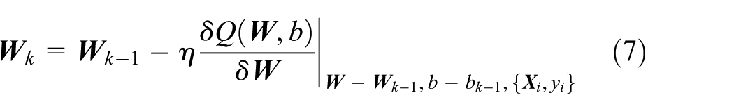
where $η$ is the learning efficiency factor.

Based on the above update formula and the OSGD³⁸ method, we can get the updated formula of the weight parameter as follows:

When $y_{t} (〈 W_{k - 1}, X_{t} 〉 + b_{k - 1}) \geq 1$

W_{k} = (1 - η) W_{k - 1}

(9)

b_{k} = b_{k - 1}

(10)

When $y_{t} (〈 W_{k - 1}, X_{t} 〉 + b_{k - 1}) < 1$

W_{k} = (1 - η) W_{k - 1} + C η y_{t} X_{t}

(11)

b_{k} = b_{k - 1} + C η y_{t}

(12)

When we use OSGD to solve the classification problem, we find that W and b may produce oscillations in the course of the iterative, that is to say that the W and b values of k – 1 are quite different from those of step k, and even they may change from positive to negative. When the number of samples is small, W and b may not reach the optimal values, so that the online learning effect is not ideal. In order to solve this problem, we first use the SVM algorithm to train the training samples before using the online support vector machine model, then get the initial W and b values, and then carry out online learning.

When the training samples are sorted by the SVM algorithm, the initial $W_{0}$ and $b_{0}$ values are close to the optimal W and b values. We hope that the $W_{k - 1}$ and $b_{k - 1}$ values of the k – 1 step are close to the $W_{k}$ and $b_{k}$ values of k step, that is, the amount of change in $W_{k}$ and $b_{k}$ should be small, they are in a gentle and stable process to achieve the best values. In order to achieve this purpose, we set the following conditions

‖ W_{k} - W_{k - 1} ‖ \leq 0.01 \times ‖ W_{k - 1} ‖

(13)

‖ b_{k} - b_{k - 1} ‖ \leq 0.01 \times ‖ b_{k - 1} ‖

(14)

That is

‖ (1 - η) W_{k - 1} + C y_{t} η X_{t} - W_{k - 1} ‖ \leq 0.01 \times ‖ W_{k - 1} ‖

(15)

‖ C η y_{t} ‖ \leq 0.01 \times ‖ b_{k - 1} ‖

(16)

Then you can get $η$

η = min (0.01 ‖ W_{k - 1} ‖ / ‖ C y_{t} X_{t} - W_{k - 1} ‖, 0.01 ‖ b_{k - 1} ‖ / ‖ C y_{t} ‖)

(17)

where $W_{k - 1}$ and $b_{k - 1}$ are the initial Lagrangian multiplier $W_{0}, b_{0}, i \in I$ after training for the SVM model. Then $η$ is

η = min (0.01 ‖ W_{0} ‖ / ‖ C y_{i} X_{i} - W_{0} ‖, 0.01 ‖ b_{0} ‖ / ‖ C y_{i} ‖)

(18)

In this article, the above algorithm is the smooth iterative online support vector machine (SIOSVM).

SIOSTM

When we want to obtain the SHTM formula, we first optimize equations (1)–(3) and obtain the following Lagrange function

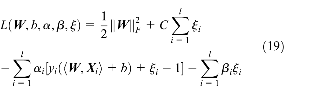
\begin{array}{l} L (W, b, α, β, ξ) = \frac{1}{2} {‖ W ‖}_{F}^{2} + C \sum_{i = 1}^{l} ξ_{i} \\ - \sum_{i = 1}^{l} α_{i} [y_{i} (〈 W, X_{i} 〉 + b) + ξ_{i} - 1] - \sum_{i = 1}^{l} β_{i} ξ_{i} \end{array}

(19)

where $α_{i} \geq 0, β_{i} \geq 0, i = 1, 2, \dots, l$ . $L (W, b, α, β, ξ)$ derivative for the variables W , b, and $ξ_{i}$ and the result is equal to zero, so we can get the following formula

W = \sum_{i = 1}^{l} α_{i} y_{i} X_{i}, \sum_{i = 1}^{l} α_{i} y_{i} = 0, 0 \leq α_{i} \leq C, i = 1, 2, \dots, l

(20)

The weight parameter W is only related to the input sample $X_{i}$ , in the case of $α_{i} \neq 0$ . Therefore, $α_{i} \neq 0$ , the input sample $X_{i}$ is the support tensor, and the sequence set of the support tensor is defined as $I = {i | α_{i} \neq 0, i = 1, 2, \dots, l}$ , then

W = \sum_{i = 1}^{l} α_{i} y_{i} X_{i} = \sum_{i \in I} α_{i} y_{i} X_{i}

(21)

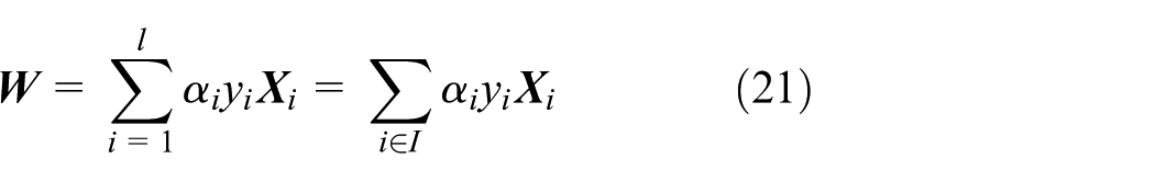
Thus, the dual problems of formulas (1)–(3) are as follows

min_{a} \frac{1}{2} \sum_{i = 1}^{l} \sum_{i = 1}^{l} a_{i} a_{j} y_{i} y_{j} 〈 X_{i}, X_{j} 〉 - \sum_{i = 1}^{l} a_{i}

(22)

s . t . \sum_{i = 1}^{l} a_{i} y_{i} = 0

(23)

0 \leq a_{i} \leq C, i = 1, 2, \dots, l

(24)

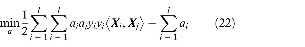
Let $X_{i} = \sum_{p = 1}^{R} x_{ip}^{(1)}, x_{ip}^{(2)}, \dots, x_{ip}^{(N)}, X_{j} = \sum_{q = 1}^{R} x_{jq}^{(1)}, x_{jq}^{(2)}, \dots, x_{jq}^{(N)}$ , you can get the following formula

\begin{matrix} 〈 X_{i}, X_{j} 〉 & \approx \sum_{p = 1}^{R} x_{ip}^{(1)}, x_{ip}^{(2)}, \dots, x_{ip}^{(N)} • \sum_{q = 1}^{R} x_{jq}^{(1)}, x_{jq}^{(2)}, \dots, x_{jq}^{(N)} \\ = \sum_{p = 1}^{R} \sum_{q = 1}^{R} 〈 x_{ip}^{(1)}, x_{jq}^{(1)} 〉 〈 x_{ip}^{(2)}, x_{jq}^{(2)} 〉 \dots 〈 x_{ip}^{(N)}, x_{jq}^{(N)} 〉 \\ = \sum_{p = 1}^{R} \sum_{q = 1}^{R} Π_{n = 1}^{N} 〈 x_{ip}^{(n)}, x_{jq}^{(n)} 〉 \end{matrix}

(25)

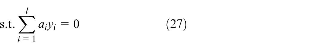
Substituting formula (25) into formulas (22)–(24) to obtain the SHTM model as follows

max_{a} \sum_{i = 1}^{l} a_{i} - \frac{1}{2} \sum_{j, k = 1}^{l} \sum_{p = 1}^{R} \sum_{q = 1}^{R} a_{j} a_{k} y_{j} y_{k} Π_{n = 1}^{N} 〈 x_{jp}^{(n)}, x_{kq}^{(n)} 〉

(26)

s . t . \sum_{i = 1}^{l} a_{i} y_{i} = 0

(27)

0 \leq a_{i} \leq C, i = 1, 2, \dots, l

(28)

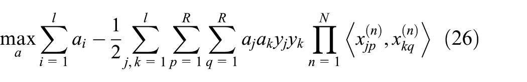
Before each update (9)–(12), it is necessary to calculate the value of $y_{t} (〈 W_{k - 1}, X_{t} 〉 + b_{k - 1})$ and compare it with the value 1 to determine the update mode of W and b.

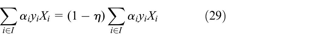
In the OSGD algorithm, each iteration needs to calculate the W . The inner product calculation of W and $X_{i}$ , which are the high-order high-dimensional tensor type, will lead to a longer calculation time, which is called “dimension disaster.” To save time costs, a can be used directly instead of W for update, and the specific steps are as follows.

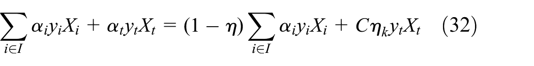
In order to make a and b values reach the optimal value quickly, the SHTM model is used to train the tensor training samples to obtain the initial $Alpha [i]_{0}$ and $b_{0}$ values, and the sequence set I consisting of support tensor.

In the iteration process, in order to avoid the values of variables a and b fluctuating frequently, the objective function can reach the optimal values in a smooth and stable way. Firstly, the learning efficiency factor was induced to perform online update calculations, whose value can be obtained by formula (18). And then the sample T was brought into the weight parameter calculation.

1. When $y_{t} (〈 W_{k - 1}, X_{t} 〉 + b_{k - 1}) \geq 1$ , the sample can be correctly classified in the current model, not the support tensor, and the tensor sequence set I remains unchanged. By formulas (9) and (21)

\sum_{i \in I} α_{i} y_{i} X_{i} = (1 - η) \sum_{i \in I} α_{i} y_{i} X_{i}

(29)

Deduce that

α_{i} = (1 - η) α_{i}, i \in I

(30)

By formula (10)

b_{k} = b_{k - 1}

(31)

2. When $y_{t} (〈 W_{k - 1}, X_{t} 〉 + b_{k - 1}) < 1$ , the sample cannot be correctly classified in the current model, there are two kinds of situations:

When the serial number t of the sample $X_{t}$ is not in the set I , the sample serial number t will be added to the set I ,³⁶ but the sample set will become more and more as time goes on until it reaches the storage capacity. So it is required to add the sequence number t of $X_{t}$ to the set I and to remove one of the samples in set I and its corresponding a value. Since the smaller the value of a, the smaller the weight of the corresponding X value, and the elimination rule is to remove the smallest value of $α_{ξ}$ and its corresponding sample $X_{ξ}$ . From formulas (11) and (21)

\sum_{i \in I} α_{i} y_{i} X_{i} + α_{t} y_{t} X_{t} = (1 - η) \sum_{i \in I} α_{i} y_{i} X_{i} + C η_{k} y_{t} X_{t}

(32)

Deduce that

α_{i} = (1 - η) α_{i}, i \in I, ξ \notin I, α_{t} = C η, I = I ⋃ {t}

(33)

By formula (12)

b_{k} = b_{k - 1} + C η y_{t}

(34)

When the serial number t of the sample $X_{t}$ is in the set I , keeping the set I unchanged. From formulas (11) and (21)

α_{i} = (1 - η) α_{i}, i \in I, i \neq t, α_{t} = (1 - η) α_{t} + C η

(35)

By formula (12)

b_{k} = b_{k - 1} + C η y_{t}

(36)

It is necessary to calculate $y_{t} (〈 W_{k - 1}, X_{t} 〉 + b_{k - 1})$ before each iteration update. However, when the tensor inner product is used to calculate the formula, the model is based on the SVM model with tensor as the training sample, so that the result is no different from the direct use of SVM. Therefore, tensor data samples are processed by canonical polyadic (CP) decomposition, which can not only reflect the spatial structure of tensor and can improve the speed of operation but also can achieve the purpose of noise reduction, which makes the calculation results more accurate and more efficient.

According to formula (25)

\begin{matrix} y_{t} (〈 W_{k - 1}, X_{t} 〉 + b_{k - 1}) = \sum_{i \in I} α_{i} y_{i} y_{t} 〈 X_{i}, X_{t} 〉 + y_{t} b_{k - 1} \\ = \sum_{i \in I} α_{i} y_{i} y_{t} (\sum_{p = 1}^{R} \sum_{q = 1}^{R} 〈 x_{ip}^{(1)}, x_{tq}^{(1)} 〉 〈 x_{ip}^{(2)}, x_{tq}^{(2)} 〉 \dots 〈 x_{ip}^{(N)}, x_{tq}^{(N)} 〉) + y_{t} b_{k - 1} \end{matrix}

(37)

Seen from formula (37), the multiplication number of CP decomposition is $(I_{1} + I_{2} + \dots + I_{N} + N - 1) \times R^{2}$ . However, the multiplication number of inner product is $I_{1} \times I_{2} \times \dots \times I_{N}$ . It is obvious that the calculation speed of the model after CP decomposition is faster. Meanwhile, the storage space of CP decomposition is $(I_{1} + I_{2} + \dots + I_{N}) \times R$ and the storage space of tensor calculation is $I_{1} \times I_{2} \times \dots \times I_{N}$ . It is clear that the CP decomposition will save a lot of storage space, which is related to R. In this paper, the value of R as set to 1.

Multi-class support tensor machine

To distinguish the normal and four cylinders in five cases, the two-class support tensor machine will be extended to multi-class support tensor machine.

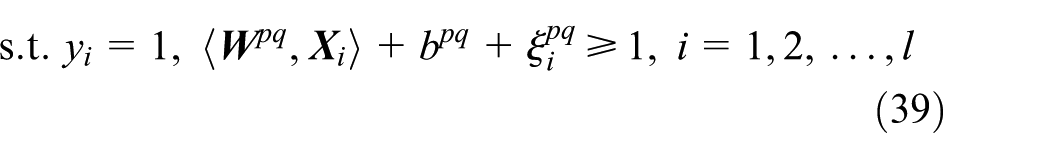
For the multi-class SVM problem, we choose one against one-SVM (OAO-SVM) algorithm. For a class c classifier problem, the algorithm needs to construct c(c – 1)/2 two-classification STM models. In this algorithm, we need to obtain the classification decision function of any two kinds of samples. For the training samples from the p and q classes, where p ≠ q, the class label corresponding to the p class is 1 and the q class is −1, and the two-class STM model is solved as follows

min_{w^{pq}, b^{pq}, ξ} \frac{1}{2} ‖ W^{pq} ‖_{F}^{2} + C \sum_{i = 1}^{l} ξ_{i}^{pq}

(38)

s . t . y_{i} = 1, 〈 W^{pq}, X_{i} 〉 + b^{pq} + ξ_{i}^{pq} \geq 1, i = 1, 2, \dots, l

(39)

y_{i} = - 1, 〈 W^{pq}, X_{i} 〉 + b^{pq} + ξ_{i}^{pq} \geq 1, i = 1, 2, \dots, l

(40)

ξ_{i}^{pq} \geq 0, i = 1, 2, \dots, l

(41)

Test sample X can be calculated using formula (41) as follows

y (x) = \arg max_{p = 1, 2, \dots, C} \sum_{q = 1, q \neq p}^{M} sgn (〈 W^{pq}, X_{i} 〉 + b^{pq})

(42)

Extender fault diagnosis method

Diagnostic process

Comprehensive use of SHTM and OSTM algorithm and the diagnosis process are shown in Figure 1. First, the extender of electric vehicles as the object, and the signals of crankshaft torque, flywheel moment of inertia, the crank pin connecting force, and connecting rod axial force were collected under its five working conditions of normal and single cylinder failure with different cylinders. Each of the signals is a function of the crank angle at different speeds, and they were used to construct the state of extender in tensor space. Then, the tensor CP decomposition algorithm is used to decompose the constructed tensor sample, and the core tensor of the extender state sample is extracted. Second, 25% samples are trained by SHTM model, and the initial Lagrange multiplier is obtained. Finally, the online algorithm of stationary iteration is used to train core tensor sample set to identify and locate the fault and compare with SVM, SHTM, and SIOSVM to verify the feasibility of SIOSTM fault diagnosis method.

Figure 1.

Flow chart of extender fault diagnosis.

Construction of extender fault tensor

Constructing state samples of range extender in tensor space, each order can be regarded as a kind of influence factor of the range extender, and each element in the tensor can be considered as the interaction results of various factors. A third-order tensor $A \in R^{I \times J \times K}$ was constructed as the state samples of the range extender. The first order $I$ of the influence factors stands for the category of the signals, including the crankshaft angular velocity, crankshaft angular acceleration, reciprocating piston inertia force, and the bearing support force. The second-order $J$ is the crank angle, and the third-order $K$ is the rotation speed which is the average speed of the crankshaft. As shown in Figure 2, the third-order tensor range extender state feature sample was constructed by “signal type $I \times$ crank angle $J \times$ rotate speed K .” Each element of the third-order tensor samples is presented as $x_{ijk}$ , where $i \in I, j \in J, k \in K$ , which represents its $j$ type signal under the rotational speed of $k$ and crankshaft angle of $i$ .

Figure 2.

Structure chart of third-order extender state sample.

Algorithm flow

The main differences between SIOSTM and SIOSVM include the training method of training samples, the update method of weight parameters, and the calculation method of inner product. For the training model of the training samples, the SIOSTM model adopts the SHTM algorithm; the training samples are the tensor samples after CP decomposition, which achieves the purpose of noise reduction and dimension reduction. However, SIOSVM model can only deal with vector input samples. So tensor pattern samples need to be expanded into vector pattern samples for training and classification, which will destroy the data structure. 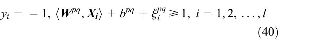For updates, SIOSTM model updates a and b, the number of updates’ times is only related to the number of initial training samples and the number of test samples, SIOSVM model updates are W and b, then it needs to do $I_{1} \times I_{2} \times \dots \times I_{n} + I_{1} \times I_{2} \times \dots \times I_{N}$ times updates, SIOSTM model updates can be more simple. For the inner product, after the CP decomposition of the SIOSTM model, the storage space and computing time are greatly reduced. For example, in this article, each sample processed by CP decomposition requires only 4 + 501 + 31 storage spaces, that is, only 536 feature attributes, and without CP decomposition requires 4 ×501 × 31 storage space, that is, 62,124 feature attributes. In general, the SIOSTM model is more suitable for complex tensor data. The steps of the SIOSTM model are shown in Table 1.

Table 1.

SIOSTM algorithm process.

Input:	The sample set $T = {X_{i}, y_{i}}_{i = 1}^{l}$ , $X_{i} \in R^{I_{I} \times I_{2} \times I_{3}}$ , $y_{i} \in {- 1 + 1}$ , maximum number of iterations J
Output:	$Alpha [i], (i = 1, 2, \dots, l)$ and b_T
Step 1:	In the sample set, 25% of the samples were selected as the training set, and trained by the SHTM model to obtain the initial $Alpha [i]_{0} (i = 1, 2, \dots, l), b_{0}$ , and the set I composed of support tensors
Step 2:	Calculate the learning efficiency $η$ according to formula (21), make k = 1
Step 3:	A sample $X_{t}$ is selected randomly from the sample set T
Step 4:	According to formulas (4)–(26): $H = y_{t} (〈 W_{k - 1}, X_{t} 〉 + b_{k - 1})$
Step 5:	If $H \geq 1$ , $b_{k} = b_{k - 1}, Alpha [i] = (1 - η) Alpha [i], i \in I$
Step 6:	If $H < 1$ , $b_{k} = b_{k - 1} + C η y_{t}$ , $Alpha [i]$ update is divided into two types: ①If $t \notin I$ , then: $Alpha [i] = (1 - η) Alpha [i], i \in I$ , $a_{ξ} = min_{i \in I} Alpha [i]$ $Alpha [t] = C η$ , $ξ \notin I, I = I \cup {t}$ ; If $t \in I$ , then: $Alpha [i] = (1 - η) Alpha [i], i \in I, i \neq t$ , $Alpha [t] = (1 - η) Alpha [i] + C η$ , $I = I$ ;
Step 7:	Let k = k + 1, if $k \leq J$ , go to step 3, otherwise, terminate the algorithm

SIOSTM: smooth iterative online support tensor machine; SHTM: support higher-order tensor machine.

Fault diagnosis results and analysis

Data acquisition

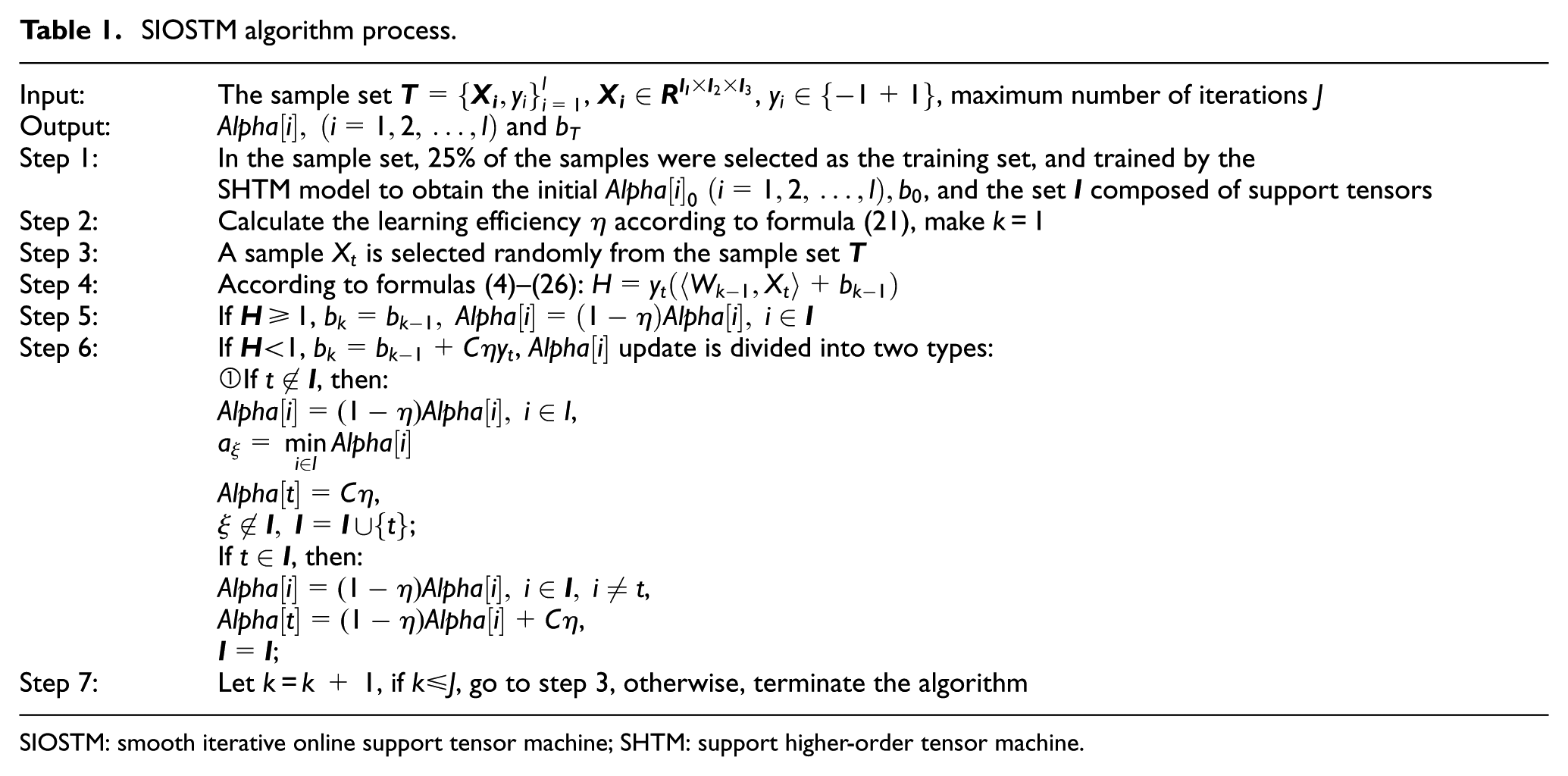
To verify the feasibility of SIOSTM in the fault diagnosis of the extended-range electric vehicle, the crankshaft angular velocity, crankshaft angular acceleration, reciprocating piston inertia force, and bearing support force of four kinds of the signals were selected as normal and misfire fault diagnosis data source. The in situ test bench and acquisition equipment are shown in Figure 3. The oil supply pipe is cut off for a short time to simulate a single cylinder misfire fault.

Figure 3.

In situ test bench.

In the process of data acquisition, the speed range of the extender is 1500–3000 r/min, the sampling interval is 100 r/min, sampling times 31 times, the sampling range 0°–720°, and the equal interval of 501 data. Therefore, 31 times sampling data of 5 states, 4 types of signals, and 16 rotational speeds are obtained. Moreover, according to the tensor type of “signal type ×crank angle × speed,” we can build 80 sizes of 4 × 501 × 31 tensor samples. According to this method, the construction of the tensor-type extender state characteristic samples are completed, and selecting randomly 20 samples as the training set, and all the sample sets are used as the test set for the verification of the diagnosis method.

Sample types

To verify the rationality of the construction method of the tensor-type extender state, the vector-type extender state sample and tensor-type sample set are input to the classification learning machine for training and diagnosis, respectively. The vector-type extender state sample set and tensor-type extender state sample set parameters are shown in Tables 2 and 3.

Table 2.

Vector state sample parameters.

The state of the extender	Number of samples	Data dimension (vector)	Number of characteristic attributes (no feature extraction)
Normal state, NS	16	1 × 62,124	62,124
Cylinder 1 Misfire, SCM1	16	1 × 62,124	62,124
Cylinder 2 Misfire, SCM2	16	1 × 62,124	62,124
Cylinder 3 Misfire, SCM3	16	1 × 62,124	62,124
Cylinder 4 Misfire, SCM4	16	1 × 62,124	62,124

Table 3.

Tensor type state sample parameters.

The state of the extender	Number of samples	Data dimension (third-order tensor)	Number of characteristic attributes
Normal state, NS	16	4 × 501 × 31	536
Cylinder 1 Misfire, SCM1	16	4 × 501 × 31	536
Cylinder 2 Misfire, SCM2	16	4 × 501 × 31	536
Cylinder 3 Misfire, SCM3	16	4 × 501 × 31	536
Cylinder 4 Misfire, SCM4	16	4 × 501 × 31	536

Experimental results analysis

The data analysis of this article uses MATLAB R2016b as the data analysis tool. The CPU used by the computer is Intel (R) Core (TM) i3-3110M 2.40 GHz, the memory is 4 GB, and the operating system is Windows 7.

In this article, the evaluation index of the algorithm is based on “test accuracy” and “learning time,” in which the learning time is taken as the average time when the algorithm runs 10 times in MATLAB. The learning time includes the training time and the estimated time of the class. The SIOSTM algorithm also includes the time of CP decomposition at R = 1, but does not include the time of building the sample and the time of the output. For all classification models, the training set consists of 25% randomly selected from all samples. To verify the stability of the SIOSTM model, different learning efficiency factors, $η$ , are chosen and compared with the learning efficiency factors calculated by formula (21). The results are shown in Table 4.

Table 4.

Accuracy rate of different learning efficiency factors $η$ .

The learning efficiency factors $η$	Accuracy rate (%)
1e–4	60
1e–5	82.5
$η$ calculated by formula (21)	96.25

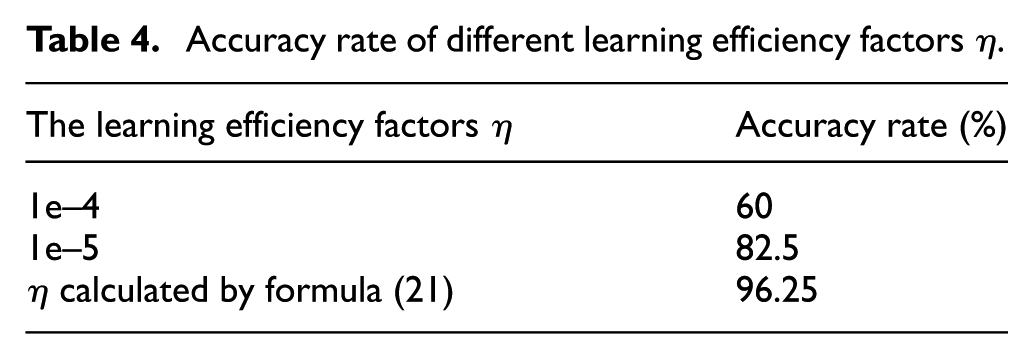
It can be seen from Table 4 that the classification accuracy of the learning efficiency factor is higher than that of the other factors because the improper learning efficiency factors will lead to oscillation of the model. Compared with the results obtained by using common learning efficiency factors, the classification accuracy of the model can be improved by using the learning efficiency factors calculated by formula (21).

The accuracy of the different learning efficiency factors $η$ is described above. Table 5 compares the accuracy of SIOSTM, SIOSVM, SHTM, and SVM models, and the accuracy rate equals the total number of samples identified divided by the total number of samples.

Table 5.

Accuracy rate of SIOSTM, SIOSVM, SHTM, and SVM models.

Classification model	Extender status	Total number of samples	Total number of samples identified	Accuracy rate (%)
SVM	NS	16	16	100
	SCM1	16	6	37.5
	SCM2	16	6	37.5
	SCM3	16	6	37.5
	SCM4	16	6	37.5
	Total	80	40	50
SIOSVM	NS	16	16	100
	SCM1	16	12	75
	SCM2	16	12	75
	SCM3	16	12	75
	SCM4	16	12	75
	Total	80	64	80
SHTM	NS	16	15	93.75
	SCM1	16	16	100
	SCM2	16	15	93.75
	SCM3	16	16	100
	SCM4	16	16	100
	Total	80	78	97.5
SIOSTM	NS	16	15	93.75
	SCM1	16	15	93.75
	SCM2	16	15	93.75
	SCM3	16	16	100
	SCM4	16	16	100
	Total	80	77	96.25

SIOSTM: smooth iterative online support tensor machine; SIOSVM: smooth iterative online support vector machine; SHTM: support higher-order tensor machine; SVM: support vector machine.

It can be seen from Table 5 that compared with the SHTM model and the SVM model, the SHTM model can correctly identify 78 samples, while the SVM model can only identify 40 samples. The accuracy of the SHTM model is 47.5% higher than that of the SVM model. Considering the classification accuracy of each state of the extender, the accuracy of the normal state of the SHTM model is slightly lower than the SVM model, while the accuracy rate of the rest of the state is much higher than that of the SVM model. So, using tensor as input samples has certain advantages in the sample classification, which can maintain the structure information of the data and achieve the purpose of noise reduction, so that the model test accuracy will be higher.

Compared with SVM and SIOSVM model, SIOSVM model can correctly identify 64 samples, while the SVM model can only correctly identify 40 samples. The accuracy of SIOSVM model is 30% higher than that of the SVM model, and the accuracy rate of each state of SIOSVM model is also higher than the SVM model. We can see that the accuracy of the model is greatly improved using the OSGD method. Therefore, online learning can not only satisfy the problem that the accuracy of the series changes with time but also can meet the problem of insufficient storage space.

The accuracy of SIOSTM model was as high as 96.25%, and the accuracy of other models was lower than SIOSTM except that the SHTM model was 1.25% higher than that of SIOSTM. Comparison of SIOSTM and SIOSVM shows that the accuracy of SIOSTM model with SIOSVM model is improved by 16.25%, and the SIOSTM model only under normal working state was about 6.25% lower than the SIOSVM model, the accurate rate of other working state is higher than the SIOSVM model, and there are even higher than about 25% SIOSVM model. What is more, the SHTM model needs to store all the samples, while the SIOSTM model only needs to store 0.25% of the samples, so that the storage space of the SIOSTM model is smaller than that of the SHTM model. Therefore, in order to solve the problems that the natural structural information may be lost and the correlation of the original data may also be broken down in vector mode, and the classification effect of offline learning mode becomes worse with time and the storage space is insufficient, this article adopts the SIOSTM model. The experimental results verify that SIOSTM can be used in the fault diagnosis of extended range. The model has a higher test accuracy and is able to maintain the effectiveness of the data changing with time and solve the storage space and other issues.

The accuracy of the different classification models is described above. Figure 4 compares the learning times of SIOSTM, SIOSVM, SHTM, and SVM models.

Figure 4.

Comparison of learning time for the four models.

As shown in Figure 4, the SIOSTM model of learning time is 5.09 s, the SHTM model of learning time is 5.59 s, the SIOSVM model of learning time is 11.25 s, and the SVM model of learning time is 9.42 s. The SIOSTM model of learning time is quicker than the SIOSVM model (6.16 s), increased by 54.76%, and the SHTM model of learning time is faster than the SVM model (3.83 s), increased by 40.66%. Therefore, the experimental results show that using tensor samples and CP decomposition will greatly shorten the learning time. In addition, the SIOSTM and SHTM models are more advantageous in terms of time when having more samples and the data dimension is higher.

According to the “test precision” and “learning time,” SIOSTM and SHTM models can achieve the purpose of noise reduction and maintain the data’s structural information and correlation. The models showed a higher test accuracy, shorter learning time, and faster convergence speed. When considering the problem of storage space, the SIOSTM model, which has more advantages, is feasible in extender fault diagnosis.

Conclusion

Lots of issues are involved in the range extender electric vehicles’ fault diagnosis, such as large samples, non-linear data, and high-dimensional data. In addition, to avoid the loss of structure information and the destruction of data dependency caused by vector input, the off-line learning algorithm often leads to the problem that the classification effect is worse with the passage of time and the storage space is not enough. In this article, we proposed the SIOSTM model to diagnose the fault parameters by combining the two algorithms of SHTM algorithm and OSGD algorithm.

The SVM, SIOSVM, SHTM, and SIOSTM algorithms were used to classify the fault parameters, and the diagnostic accuracy and model learning time were used as the evaluation indexes. The experimental results show that the accuracy rate of SIOSTM model is 96.25%, except that the SHTM model is 1.25% higher than SIOSTM, and the accuracy of the other models is lower than SIOSTM. In terms of learning time, the SIOSTM model only needs 5.09 s, which is the shortest time in all classification models. In addition, the SIOSTM model can solve the problem of storage space as it only needs to store 0.25% of the samples.

In summary, the fault diagnosis method based on the SIOSTM can not only reduce the noise but also maintain the data’s structural information and correlation, which makes the diagnosis model more accurate, faster convergence speed, and shorter learning time. At the same time, the fault diagnosis method based on SIOSTM model can do online learning under the premise of ensuring classification accuracy and solves the problem of data storage capacity. Therefore, it is feasible to apply the SIOSTM model to the fault diagnosis of electric vehicle range extender.

Footnotes

Handling Editor: Zhixiong Li

Declaration of conflicting interests

The author(s) declared no potential conflicts of interest with respect to the research, authorship, and/or publication of this article.

Funding

The author(s) disclosed receipt of the following financial support for the research, authorship, and/or publication of this article: This work was supported by the National Natural Science Foundation of China under Grant No. 51505345 and Grant No. 51509194, the Science & Technology Research Project of Education Department of Hubei Province under Grant No. Q20151105, and the open fund of Hubei Key Laboratory of Mechanical Transmission and Manufacturing Engineering at Wuhan University of Science and Technology under Grant No. 2017A12.

ORCID iD

Xiaowei Xu

References

Wahono

Santoso

Nur

. Analysis of range extender electric vehicle performance using vehicle simulator. Enrgy Proced 2015; 68: 409–418.

Borghi

Mattarelli

Muscoloni

. Design and experimental development of a compact and efficient range extender engine. Appl Energ 2017; 202: 507–526.

Wang

Zhang

. Review of the fault mechanism and diagnostic techniques for the range extender hybrid electric vehicle. IEEE Access 2017; 5: 14234–14244.

Lee

Ahn

Park

. A fault diagnosis expert system for distribution substations. IEEE T Power Deliver 2000; 15: 92–97.

Ratcliff

Dane

Williams

. Diesel particle filter and fuel effects on heavy-duty diesel engine emissions. Environ Sci Technol 2010; 44: 8343–8349.

Pan

Zhang

. Multi-sensor information fusion method and its applications on fault detection of diesel engine. In: International conference on computer science and network technology, Harbin, China, 24–26 December 2011, vol. 4, pp.2551–2555. New York: IEEE.

Xia

Zhang

. Research of condenser fault diagnosis method based on neural network and information fusion. In: International conference on computer and automation engineering, Singapore, 26–28 February 2010, vol. 5, pp.709–712. New York: IEEE.

Zhan

Wei

Huo

. Research on delamination fault diagnosis of marine diesel engine based on support vector machine. In: IEEE international symposium on industrial electronics, Seoul, South Korea, 5–8 July 2009, vol. 20, pp.1224–1227. New York: IEEE.

Tao

. Supervised tensor learning. Knowl Inf Syst 2007; 13: 1–42.

10.

Hao

Chen

. A linear support higher-order tensor machine for classification. IEEE T Image Process 2013; 22: 2911–2920.

11.

Liu

Guo

. A low-rank approximation-based transductive support tensor machine for semisupervised classification. IEEE T Image Process 2015; 24: 1825–1838.

12.

Gastaldo

Pinna

Seminara

. A tensor-based pattern-recognition framework for the interpretation of touch modality in artificial skin systems. IEEE Sens J 2014; 14: 2216–2225.

13.

Takallou

Kasaei

. Head pose estimation and face recognition using a non-linear tensor-based model. IET Comput Vis 2014; 8: 54–65.

14.

Chen

Wang

Zhong

. One-class support tensor machine. Knowl-Based Syst 2016; 96: 14–28.

15.

Sidiropoulos

Lathauwer

. Tensor decomposition for signal processing and machine learning. IEEE T Signal Proces 2017; 65: 3551–3582.

16.

Mordohai

Medioni

. Tensor voting: a perceptual organization approach to computer vision and machine learning (Synthesis lectures on image video & multimedia processing), vol. 2. San Rafael, CA: Morgan & Claypool Publishers, 2006, 136p.

17.

Zhang

. Global existence and the optimal decay rates for the three dimensional compressible nematic liquid crystal flow. Acta Appl Math 2017; 150: 67–80.

18.

Cavallanti

Cesa-Bianchi

Gentile

. Tracking the best hyperplane with a simple budget perceptron. Mach Learn 2007; 69: 143–167.

19.

Kivinen

Smola

Williamson

. Online learning with kernels. IEEE T Signal Proces 2004; 52: 2165–2176.

20.

Lau

. Online training of support vector classifier. Pattern Recogn 2003; 36: 1913–1920.

21.

Orabona

Castellini

Caputo

. On-line independent support vector machines. Pattern Recogn 2010; 43: 1402–1412.

22.

Zhao

Hoi

SCH

Jin

. Double updating online learning. J Mach Learn Res 2011; 12: 1587–1615.

23.

Auer

Cesa-Bianchi

Gentile

. Adaptive and self-confident on-line learning algorithms. J Comput Syst Sci 2002; 64: 48–75.

24.

Bollegala

. Dynamic feature scaling for online learning of binary classifiers. Knowl-Based Syst 2017; 129: 97–105.

25.

Rasilo

Räsänen

. An online model for vowel imitation learning. Speech Commun 2017; 86: 1–23.

26.

Weel

D’Angelo

Haasdijk

. Online gait learning for modular robots with arbitrary shapes and sizes. Artif Life 2017; 23: 80–104.

27.

Yan

Yang

. Multilinear discriminant analysis for face recognition. IEEE T Image Process 2007; 16: 212–220.

28.

Plataniotis

Venetsanopoulos

. Color image processing and applications, vol. 12. Berlin: Springer, 2001, p.222.

29.

Negi

Labate

. 3-D discrete shearlet transform and video processing. IEEE T Image Process 2012; 21: 2944–2954.

30.

Chellappa

Roy-Chowdhury

Zhou

. Recognition of humans and their activities using video (Synthesis lectures on image video & multimedia processing), vol. 1. San Rafael, CA: Morgan & Claypool Publishers, 2005, 173p.

31.

Plataniotis

Venetsanopoulos

. MPCA: multilinear principal component analysis of tensor objects. IEEE T Neural Networ 2008; 19: 18–39.

32.

Renard

Bourennane

. Dimensionality reduction based on tensor modeling for classification methods. IEEE T Geosci Remote 2009; 47: 1123–1131.

33.

Wang

Ahuja

. Compact representation of multidimensional data using tensor rank-one decomposition. In: International conference on pattern recognition, Cambridge, 26 August 2004, vol. 1, p.44–47. New York: IEEE.

34.

Bengua

Phien

Tuan

. Efficient tensor completion for color image and video recovery: low-rank tensor train. IEEE T Image Process 2017; 26: 2466–2479.

35.

Zhou

Yang

Guangchao

. Online support tensor machine. J Front Comput Sci Technol 2013; 7: 611–619.

36.

Zhao

Zhou

Adali

. Kernelization of tensor-based models for multiway data analysis: processing of multidimensional structured data. IEEE Signal Proc Mag 2013; 30: 137–148.

37.

Wang

Fang

Liu

. Stochastic compositional gradient descent: algorithms for minimizing compositions of expected-value functions. Math Program 2017; 161: 1–31.

38.

Wang

Crammer

Vucetic

. Breaking the curse of kernelization: budgeted stochastic gradient descent for large-scale SVM training. J Mach Learn Res 2012; 13: 3103–3131.

Smooth iteration online support tension machine algorithm and application in fault diagnosis of electric vehicle extended range

Abstract

Keywords

Introduction

SIOSTM

Smooth iterative online support vector machine

SIOSTM

Multi-class support tensor machine

Extender fault diagnosis method

Diagnostic process

Construction of extender fault tensor

Algorithm flow

Fault diagnosis results and analysis

Data acquisition

Sample types

Experimental results analysis

Conclusion

Footnotes

Declaration of conflicting interests

Funding

ORCID iD

References