Sage Journals: Discover world-class research

Abstract

This study aims to propose and investigate a theoretical maximum traffic flow method. Furthermore, we propose a merging timing control based on the results obtained from this method, which are verified using actual automated guided vehicles. The results (micro-level optimization) enable automated guided vehicles to achieve a fabrication level optimization (macro-level optimization). Engineers working in the field of automated guided vehicles have found that there is an optimal headway distance that achieves a maximum traffic throughput when automated guided vehicles operate with merging points. “Zipper merging” is known to be a suitable merging method resulting from “Jamology.” In this study, first, we will verify the results using the “Zipper merging” simulation model. Second, we develop a mathematical model and verify its simulations and experiments using actual automated guided vehicles. Finally, we develop a merging timing control to augment transfer flow and verify the effects using a small full fabrication simulation. We predict that this control will improve factory model throughput when used in practical applications.

Keywords

Industrial application automated guided vehicle Jamology control engineering modeling

Introduction

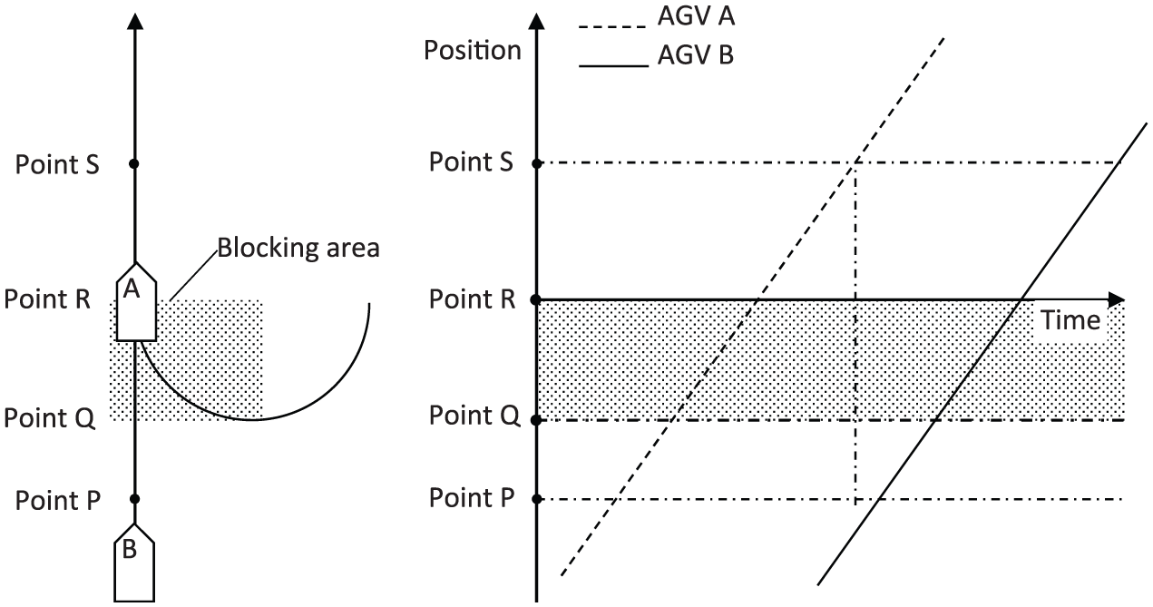
In semiconductor industries, wafers are processed using various pieces of equipment and transferred between equipment by automated guided vehicles (AGVs) in an automated material handling system (AMHS).¹ In this study, transfer refers to the movement of wafers, whereas traffic refers to AGV movement. AGVs operate along rails in the AMHS (see Figure 1), which includes numerous intersections, such as merging and diverging points. The rails consist of segments, which are the sections between two points, as shown in Figure 2. Blocking area consists of two segments at an intersection. Only one AGV can enter a blocking area at a time to avoid collisions with the other AGVs. AGVs without permission must stop at the entrance of the blocking area. Thus, traffic jams occur at intersections where there is a gathering of AGVs, as shown in Figure 3. Therefore, researchers are aware that there is a limit to the number of AGVs that can approach a merging point, which lessens the number of traffic jams.

Figure 1.

AMHS and the essential parts of the system.

Figure 2.

The relationship between segments and the blocking area.

Figure 3.

A schematic showing the occurrence of traffic jams at a merging point.

Several methods have been proposed to analyze and/or control the entire transportation system. These methods can be categorized into three approaches, which are simulation, statistical, and optimization based. The simulation-based approach is one of the most popular methods currently in practice.^2,3 This approach is extremely time-consuming because it requires high model detail as well as several trials and errors to obtain a good result. This problem has been solved using generic models.⁴ However, a good result does not always reflect true best performance because it is a result of trials and errors. Queueing network theory and Markov models are often used as a statistical approach.^5,6 These methods provide good results for mean performance values, such as transportation throughput, but do not provide the maximum performance values either. Previous studies have modeled AGV systems as resource-oriented petri nets or integer linear programming problems, which are categorized as the optimization approach.^7–9 These methods provide a maximum theoretical performance. However, the processing time can be too long for use in a large semiconductor factory. An AGV system has been modeled as a linear programming problem to reduce the processing time but provides a maximum theoretical throughput.¹⁰ To achieve a maximum theoretical throughput, the method requires that AGVs have a maximum throughput at the merging and loading/unloading points. However, this study does not provide the maximum throughput at merging points, which was one of the challenges in this study.

After determining the maximum throughput, we must find a method to achieve it practically. To control AGV throughput at merging points, the timing of AGVs entering the merging points should be controlled, which is the second challenge in this study. Solutions to this problem can be divided into three approaches: (1) the optimal scheduling approach,¹¹ (2) the control theory–based approach,¹² and (3) the simulation-based and/or statistical approach.^13–15 In a study, AGVs were modeled around a merging point as an integer linear programming problem, providing AGV schedules, which describe AGV movement.¹¹ AGVs, however, cannot maintain the schedule due to modeling errors caused by certain methods that divide continuous rails into discrete sections. AGV trajectory control was provided to avoid AGV collisions.¹² Although it is a good method, the AMHS scenario from this previous study is different from the scenario in this study. For example, there are blocking areas, which are not defined in the study, in the AMHS that accept only one AGV. Queueing network theory and Markov models were used as the statistical approach.¹³ In this study, vehicles decide whether to stop or go at merging points. However, AGVs can be fully controlled by an upper-level controller in this study. There is now a new approach to analyze and solve traffic jams, called “Jamology.”¹⁴“Jamology” provides important information about traffic jams. For example, it provides information about the relationship between AGV density and road traffic flow and that zipper merging is effective at merging points.¹⁵ Our previous study provided methods to encourage maximum traffic flow by applying the principles of “Jamology” to AMHS.¹⁶ AGVs were considered as a self-driven particle, which suggests that AGVs move as they wish.^13–15 On the other hand, AGVs are regulated by an upper-level controller. Our previous study considers these differences.

This article builds on previous models to obtain maximum traffic flow in actual AMHSs. The model is not only verified with simulations but also with actual AGV experiments. Furthermore, a merging timing control method is developed to utilize the models in actual scenarios. This method is evaluated via simulations to observe whether it augments the semiconductor fabrication transfer flow.

Traffic jam analysis

Problem definition

AGV specification

AGVs run along pre-installed rails as shown in Figure 1. AGV length and velocity are expressed as non-negative values, that is, $l_{v}$ and $v \leq v_{\max}$ , respectively. AGV dynamics are described using a simple kinematic equation

\overset{\cdot}{v} = u

(1)

where u is the control input (m/s²) defined as $u = - d$ if $x < l_{h}$ and $v > 0$ , $u = 0$ if $x < l_{h}$ and $v = 0$ , $u = 0$ if $x \geq l_{h}$ and $v = v_{\max}$ , and $u = a$ if $l \geq l_{h}$ and $v < v_{\max}$ when the control target AGV is not around a merging point. x is the actual headway distance between two consecutive AGVs and $l_{h}$ is the safe headway distance. AGVs respond rapidly to acceleration commands. Thus, we do not include delays associated with commands in equation (1) in this study. AGVs communicate with each other based on the communication processing time, $T_{c}$ (see Tables 1 and 2 and Figure 4).

Table 1.

AGV specifications.

Definition	Variable
Length (m) of AGV	$l_{v} (> 0)$
Inter-vehicular distance (m) between stopped AGVs, which is the distance between the front edge of an AGV and the rear edge of the front AGV	$l_{a} (\geq 0)$
Safe inter-vehicular distance (m) when AGVs have a velocity v (AGVs cannot run with an inter-vehicular distance shorter than this)	$l_{s} (v) (= \frac{v^{2}}{2 d} + l_{a})$
Safe headway distance when AGVs have a velocity v (m) (headway distance is the distance between the front edge of an AGV and the front edge of the front AGV)	$l_{h} (v) (= l_{s} (v) + l_{v})$
Actual headway distance between the AGV and the front AGV, which is regulated so that $x \geq l_{h} (v)$	x
Maximum velocity (m/s) of an AGV (AGVs run with maximum velocity unless prohibited to enter a blocking area or if the AGV is likely to violate the safe headway distance)	$v_{\max}$
Actual velocity (m/s) of an AGV	$v (\geq 0, \leq v_{\max})$
Acceleration (m/s²) of an AGV	$a (> 0)$
Deceleration (m/s²) of an AGV	$d (> 0)$
Communication processing time (s), which is the amount of time needed for AGVs to communicate	$T_{c} \geq 0$

AGV: automated guided vehicle.

Table 2.

Certain AGV conditions and the appropriate decision to avoid AGV collisions.

Condition			Decision
Position of a control target AGV	Position of the front AGV	v of the control target AGV	u of the controltarget AGV
There is an AGV outside of the section between points P and Q (the definitions of points P and Q are shown in section “Specification of AGV behavior around blocking areas”)	The front AGV is at a position satisfying $x < l_{h}$	$v > 0$	$u = - d$
	The front AGV is at a position satisfying $x < l_{h}$	$v = 0$	$u = 0$
	The front AGV is at a position satisfying $x \geq l_{h}$	$v = v_{\max}$	$u = 0$
	The front AGV is at a position satisfying $x \geq l_{h}$	$v < v_{\max}$	$u = a$

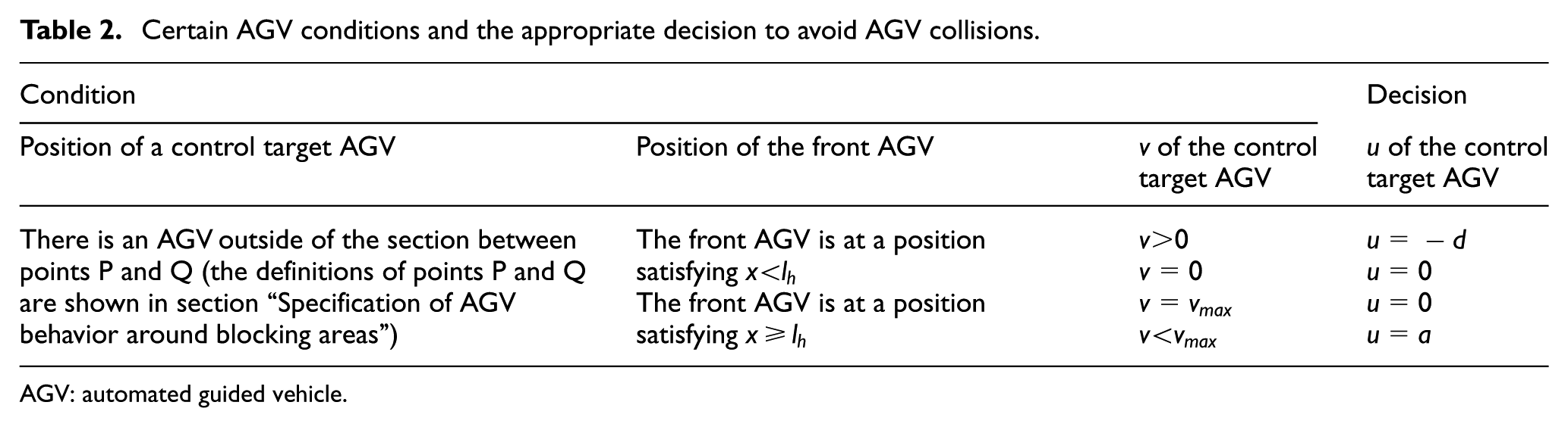
AGV: automated guided vehicle.

Figure 4.

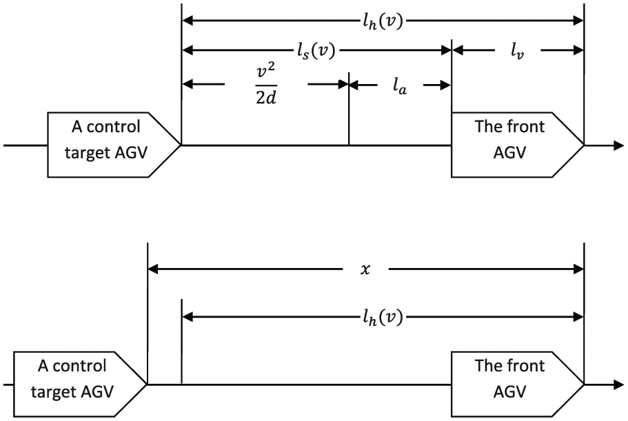
The relationship between distances involved with AGVs.

Specification of AGV behavior around blocking areas

Figure 5 illustrates a scenario where AGVs are merging into a blocking area. Blocking areas are positioned at all merging points. A blocking area allows only one AGV to enter at a time so as to avoid AGV collisions. Points Q1 and Q2 are entrances and point R is an exit. $l_{b 1}$ and $l_{b 2}$ are the lengths of the blocking area.

Figure 5.

A scenario where AGVs merge into a blocking area.

To enter a blocking area, an AGV must have permission. There is only one permission at a merging point. The distance between point P1 or P2 and point Q1 or Q2 is the AGV braking distance, such that $v^{2} / 2 d$ . When AGV B has permission at point P, it can enter the blocking area without decelerating (see Figure 6). However, AGV B must begin to decelerate at point P1 or P2 if it does not receive permission. When AGV B gains permission during deceleration (see Figure 7) or while waiting at point Q1 or Q2 (see Figure 8), it begins to reaccelerate. After AGV A exits the blocking area, it relinquishes permission, but it takes a certain amount of time for AGV B to receive permission after AGV A relinquishes permission. This time period is known as the “Communication processing time” in this study. We assume that the length of the blocking area is sufficiently large for the AGV to accelerate to the maximum velocity, $v_{\max}$ , within this area. Thus, we can modify Table 2 and construct Table 3 where x is defined virtually as shown in Figure 9.

Figure 6.

AGV B trajectory when AGV B is permitted to enter the blocking area when the AGV arrives at point P.

Figure 7.

AGV B trajectory when AGV B is permitted to enter the blocking area during AGV deceleration.

Figure 8.

AGV B trajectory when AGV B is permitted to enter the blocking area when the AGV stops.

Table 3.

Decisions to avoid AGV collisions.

Condition			Decision
Position of a control target AGV	Position of the front AGV	v of the control target AGV	u of the control target AGV
There is an AGV outside thesection between points P and Q	The front AGV is at a positionthat satisfies $x < l_{h}$	$v > 0$	$u = - d$
	The front AGV is at a positionthat satisfies $x < l_{h}$	$v = 0$	$u = 0$
	The front AGV is at a positionthat satisfies $x \geq l_{h}$	$v = v_{\max}$	$u = 0$
	The front AGV is at a positionthat satisfies $x \geq l_{h}$	$v < v_{\max}$	$u = a$
There is an AGV in the sectionbetween points P and Q	There is a front AGV in the section between points P and R	$v > 0$	$u = - d$
	There is a front AGV in the section between points P and R	$v = 0$	$u = 0$
	There is a front AGV in a sectionfarther than point R	$v = v_{\max}$	$u = 0$
	There is a front AGV in a sectionfarther than point R	$v < v_{\max}$	$u = a$

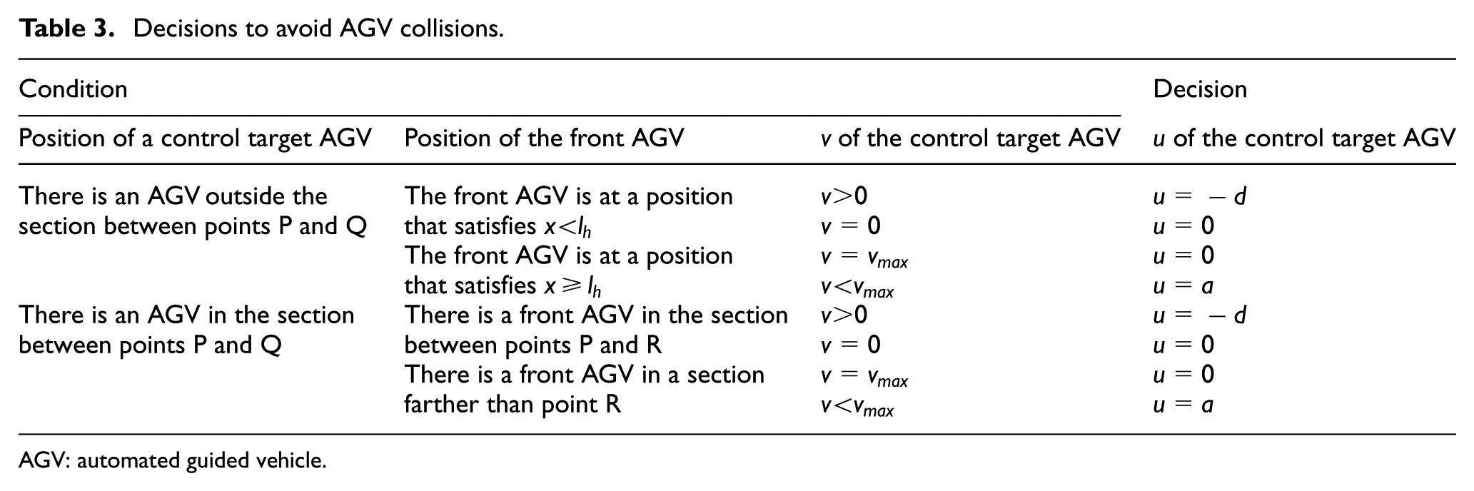
AGV: automated guided vehicle.

Figure 9.

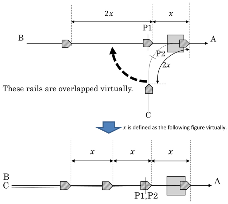
Headway distance, x, defined virtually around a merging point.

Traffic flow comparison at a merging point

AGV system controller engineers at Murata Machinery empirically know that traffic jams occur if x is too small at merging points. In this section, we verify the knowledge from their experiences by simulations that are modeled as scenarios around a merging point. AGVs disappear in the lower section of the merging point in the simulation. Thus, traffic jams downstream of the merging point do not occur and do not affect traffic around the merging point. Figures 10 –12 illustrate situations where x is defined as 4.040, 2.820, and 1.000 m, respectively. The other conditions are listed in Table 4.

Figure 10.

Simulation at $v = 1.010 m / s$ and $x = 4.040 m$ .

Figure 11.

Simulation at $v = 1.010 m / s$ and $x = 2.82 m$ .

Figure 12.

Simulation at $v = 1.010 m / s$ and $x = 1.0 m$ .

Table 4.

Conditions for traffic flow analysis at a merging point.

Variables		Values
$l_{v}$		0.700
$l_{a}$		0.300
$v_{\max}$		1.010
a		0.500
d		1.000
$l_{b 1}$ , $l_{b 2}$		2.300, 2.300
$T_{c}$	Mean set	0.000
$T_{c}$	Standard deviation set	0.000

Out of the three scenarios, it can be seen from Figure 11 that the headway distance, after the merging point, is the shortest.

We model two types of simulations in this section: (1) with only two AGVs (see Figure 13) and (2) with multiple AGVs for 1 min (see Figure 14). The inverse of the time period between AGVs at the blocking area exit is measured as traffic flow $F (1 / s)$ . Figure 15 shows the relationship between traffic flow, x, and F. Circles are traffic flows similar to Figure 13. Rhomboids are traffic flows similar to Figure 14. In the former case, AGVs do not decelerate when $x \geq 2.828$ . AGVs decelerate but begin to reaccelerate during deceleration when $2.828 > x \geq 1.881$ . AGVs decelerate and stop, to wait for permission, when $1.881 > x$ . In the latter case, AGVs do not decelerate when $x \geq 2.828$ . AGVs decelerate but start to reaccelerate during the deceleration when $2.828 > x \geq 2.727$ . AGVs decelerate and stop, to wait for permission, when $2.727 > x$ . When multiple AGVs operate with a headway distance $2.727 \geq x \geq 1.881$ , which continues to affect the other AGVs in the queue until permission is granted and all AGVs pass. On the other hand, front AGVs delay rear AGVs more when $2.727 > x$ . Eventually, rear AGVs must stop at point Q, similar to AGVs in the latter case. The traffic jam cannot be cleared because AGVs continuously come from the upper stream. The range of $2.727 > x \geq 1.881$ is identical to the meta-stable characteristic in “Jamology.”¹¹ These simulations indicate that zipper merging is an efficient merging style at merging points.¹²

Figure 13.

Traffic flow with two operating AGVs.

Figure 14.

Traffic flow with multiple AGVs operating for 1 min.

Figure 15.

Simulation results with various x parameters.

AGV model behavior development around a merging point

Simulations in section “Traffic flow comparison at a merging point” show that AMHS AGVs conform to the results of “Jamology.”“Jamology” proposes the concept of “Zipper merging,”¹² which is a merging style where only one AGV enters a merging point, thus improving the AGV flow. This study uses this merging style as shown in Figure 9. In addition to this, this study considers that AGVs have a finite acceleration and deceleration and that AGVs’ positions are controlled by the AMHS controller. Thus, this study focuses on the relationships between AGV headway distance, x (m), and AGV traffic flow, F (1/s).

A rail is virtually superimposed on the other rail to define the headway distance between merging AGVs as shown in Figure 9. P1 and P2 are the limit points for AGVs operating with a velocity, v, in order to stop at the blocking area entrance. Here x is treated as the headway distance between the front and the rear AGV when the rear AGV is at the limit point P1 or P2. x cannot be smaller than the safe headway distance, $l_{h} (v)$ . Traffic flow, F (1/s), is defined as the number of AGVs that pass through the blocking area exit every second.

We develop, for several cases, the mathematical model that provides a relationship between x and F as follows

Case 1. $x \geq l_{b} + (v_{\max}^{2} / 2 d) + v_{\max} T_{c}$

In this case, rear AGVs, which arrive at P1 or P2, are permitted to enter the blocking area because the front AGVs have already finished communication and passed permission to the rear AGV. Thus, traffic flow is written as

F (v) = \frac{v}{x}

(2)

Case 2. $l_{b} + (v_{\max}^{2} / 2 d) + v_{\max} T_{c} > x$

In this case, rear AGVs are not permitted to enter the blocking area because front AGVs are still operating in the area. Thus, rear AGVs decelerate until they receive permission. Front AGVs exit the blocking area while rear AGVs decelerate. Just after the front AGVs relinquish permission to the rear AGVs, the rear AGVs reaccelerate until they have reached a maximum velocity, $v_{\max}$ .

In this case, the behavior when the number of AGVs is quite small (see Figure 13) is different compared with a case where there are a large number of AGVs (see Figure 14). Thus, we divide this case into Cases 2-1 and 2-2:

Case 2-1. A small number of AGVs approach a merging point

(I) x \geq l_{b} + v_{\max} T_{c} - \frac{v_{\max}^{2}}{2 d}

In this case, front AGVs relinquish permission while rear AGVs decelerate. Thus, rear AGVs begin to reaccelerate before they completely come to a stop. The transfer flow can be obtained using basic Newtonian mechanics

F (v) = \frac{v_{\max}}{k {(L - x)}^{2} + x}

(3)

where $L = l_{b} + (v_{\max}^{2} / 2 d) + v_{\max} T_{c}$ and $k = d (a + d) / 2 {av}_{\max}^{2}$

(II) l_{b} + v_{\max} T_{c} - \frac{v_{\max}^{2}}{2 d} > x

In this case, front AGVs relinquish permission after rear AGVs have stopped to wait at the entrance. We can calculate the transfer flow using basic Newtonian mechanics

F (v) = \frac{v_{\max}}{l_{b} + v_{\max} T_{c} + \frac{v_{\max}^{2}}{2 a}}

(4)

Case 2-2. Multiple AGVs approach a merging point

This case is the focus of our study, that is, the situation where AGVs rush to a merging point

(I) x \geq L - \frac{{av}_{\max}^{2}}{2 d (a + d)}

In this case, front AGVs relinquish permission while rear AGVs decelerate, and front AGVs do not delay rear AGVs more than the front AGVs have been delayed. Considering the above constraints, we obtain the transfer flow from equation (3)

(II) L - \frac{{av}_{\max}^{2}}{2 d (a + d)} > x

In this case, the front AGVs cause the rear AGVs to have more delay than their own delay. Thus, the rear AGVs must completely stop until all of the front AGVs relinquish permission. We obtain the transfer flow using basic Newtonian mechanics, such as in equation (4).

AGV model verification

We verify the model obtained in section “AGV model behavior development around a merging point” with both simulations and experiments.

Verification with simulation

Simulation conditions

We conducted two types of simulations, which are shown in Figure 16. The layout is identical to section “Traffic jam analysis.” Conditions are also identical to those listed in Table 4. In the simulation, AGVs disappear in the lower section of the merging point. Thus, traffic jams downstream of the merging point do not occur and do not affect traffic around the merging point.

Figure 16.

The layout of the experimental environment.

Simulation results

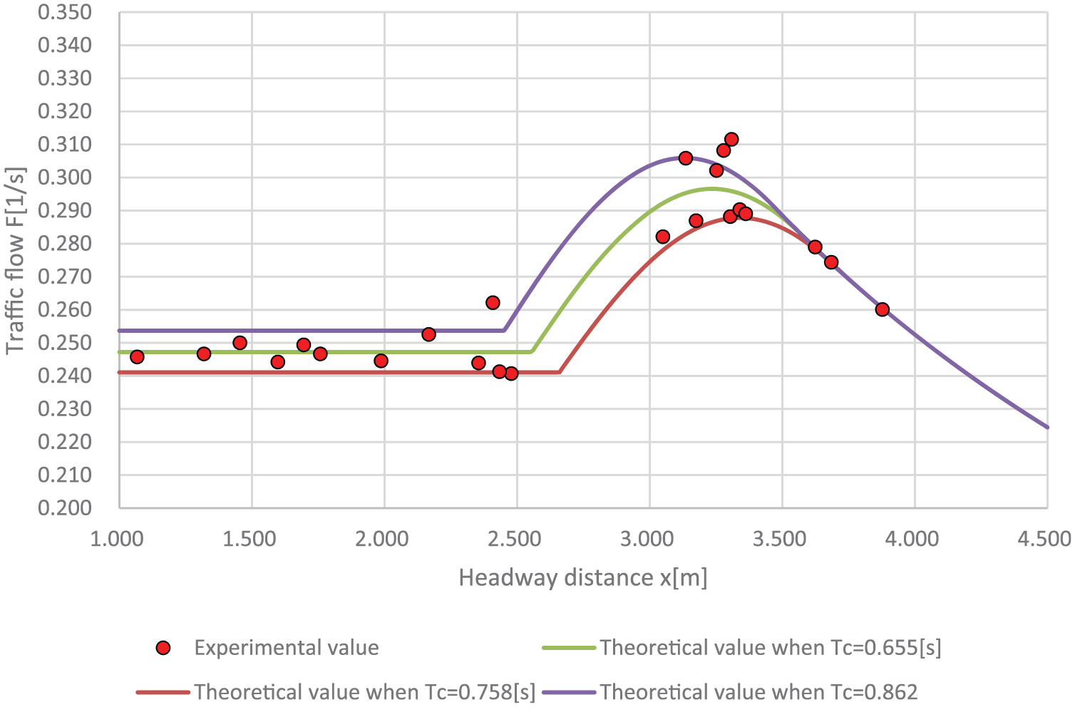
Simulations were conducted using the AutoMod^™ simulation software.¹⁷ Figure 17 plots the simulation results and theoretical values.

Figure 17.

Theoretical value verification via simulations.

When simulating only two operating AGVs, the transfer flow follows equation (2) when $x \geq 2.811 m$ , equation (3) when $2.811 m > x \geq 1.790 m$ , and equation (4) when $1.790 m > x$ .

When simulating multiple AGVs for a period of 1 min, the transfer flow follows equation (2) when $x \geq 2.811 m$ , equation (3) when $2.811 m \geq x \geq 2.641 m$ , and equation (4) when $2.641 m > x$ . The headway distance, x, should be controlled when $2.641 m \geq x \geq 2.811 m$ in order to improve traffic flow. It is very important to note that the headway distance should be no smaller than $2.641 m$ because distances smaller than this cause traffic jams.

Based on these results, we observe that the model developed in section “AGV model behavior development around a merging point” clearly explains the simulation results.

Verification with actual AGVs

Experimental conditions

Experiments were conducted at a test site at Murata Machinery, Ltd (see Figure 18) under the conditions listed in Table 5. Communication processing time is different compared with the simulations. We only conduct the two-operating AGV case due to constraints based on the number of AGVs at the test site.

Figure 18.

Experimental environment layout.

Table 5.

Experimental conditions.

Variables	Values	Value conditions
$l_{v}$	0.700	Designed
$l_{a}$	0.300	Set
$v_{\max}$	1.010	Set
a	0.500	Set
d	1.000	Set
$l_{b 1}$	2.300	Designed
$T_{c}$	0.758	Mean of measured
$T_{c}$	0.103	Standard deviation of measured

Experimental results

Experimental results are listed in Table 6 and experimental results and theoretical values are plotted together in Figure 19. Theoretical values are also plotted where $T_{c} = m e a n - s t a n d a r d d e v i a t i o n (= 0.655 s)$ , $T_{c} = mean (= 0.758 s)$ , and $T_{c} = m e a n + s t a n d a r d d e v i a t i o n (= 0.862 s)$ . We observe that nearly all experimental results are within the range of the theoretical values, with only three exceptional points: $(2.409 m, 0.262 1 / s), (3.279 m, 0.308 1 / s), and (3.309 m, 0.312 1 / s)$ . $T_{c}$ is 0.535 s when $x = 3.279 m$ and $T_{c}$ is 0.520 s when $x = 3.309 m$ . These communication processing times are smaller than the $mean - standard deviation (0.655 s)$ . Thus, traffic flow is larger than the theoretical value when $T_{c} = 0.655 s$ . We were unable to understand the reason for which traffic flow is larger than the theoretical value when $x = 2.409 m$ . We consider that this experimental result, $x = 2.409 m$ , includes some error. When equation (1) was created, delays associated with commands were ignored because they were very small. Communication processing time is the time period from the time when a front AGV exits the blocking area to the time when a rear AGV starts to accelerate. Thus, the time period must include delays.

Table 6.

Experimental results.

Experiment no.	Experiment time		x (m)	T_c (s)	The front AGV passing timeat point 108 (ms)	The rear AGVpassing timeat point 108 (ms)	Passing timespan (s)	Experimentalvalue of trafficflow (1/s)
Experiment no.	Date	time	x (m)	T_c (s)	The front AGV passing timeat point 108 (ms)	The rear AGVpassing timeat point 108 (ms)	Passing timespan (s)	Experimentalvalue of trafficflow (1/s)
1	15 June 2017	16:31:55	3.252	0.715	17,065	20,375	3.31	0.302
2	15 June 2017	16:34:56	2.478	0.855	17,830	21,985	4.16	0.241
3	15 June 2017	16:36:11	2.434	0.845	18,030	22,175	4.15	0.241
4	15 June 2017	16:37:23	3.624	0.840	17,880	21,465	3.59	0.279
5	15 June 2017	16:38:36	3.175	0.860	18,315	21,800	3.49	0.287
6	15 June 2017	16:39:50	3.309	0.520	17,985	21,195	3.21	0.312
7	15 June 2017	16:41:03	3.279	0.535	15,485	18,730	3.25	0.308
8	15 June 2017	16:42:15	3.304	0.875	18,125	21,595	3.47	0.288
9	15 June 2017	16:43:33	1.987	0.820	18,080	22,170	4.09	0.244
10	15 June 2017	16:44:48	2.167	0.725	18,005	21,965	3.96	0.253
11	15 June 2017	16:45:23	1.758	0.785	17,725	21,780	4.06	0.247
12	15 June 2017	16:46:36	1.598	0.760	17,655	21,750	4.10	0.244
13	15 June 2017	16:46:36	1.695	0.675	17,430	21,440	4.01	0.249
14	15 June 2017	16:47:47	1.455	0.670	18,075	22,075	4.00	0.250
15	15 June 2017	16:48:24	1.067	0.735	17,385	21,455	4.07	0.246
16	15 June 2017	16:49:01	1.319	0.725	16,975	21,030	4.06	0.247
17	15 June 2017	16:55:03	3.878	Unknown	16,020	19,865	3.85	0.260
18	15 June 2017	16:55:40	2.355	0.805	17,530	21,630	4.10	0.244
19	15 June 2017	16:56:13	3.050	0.845	17,340	20,885	3.55	0.282
20	15 June 2017	16:56:49	3.136	0.680	17,485	20,755	3.27	0.306
21	15 June 2017	16:57:59	3.340	0.860	17,625	21,070	3.45	0.290
22	15 June 2017	16:58:35	2.409	0.675	17,645	21,460	3.82	0.262
23	15 June 2017	16:59:09	3.362	0.875	17,140	20,600	3.46	0.289
24	15 June 2017	16:59:44	3.685	Unknown	17,300	20,945	3.65	0.274

AGV: automated guided vehicle.

Figure 19.

Experimental and theoretical values.

The verification of the two operating AGVs and multiple operating AGVs for 1-min simulations proves that the model developed in section “AGV model behavior development around a merging point” is feasible. Unfortunately, only the experiment with two operating AGVs was completed due to constraints on the number of AGVs at the test site. These verifications prove that the model developed in section “AGV model behavior development around a merging point” is applicable to real-world situations. We consider that the model developed in section “AGV model behavior development around a merging point” is sufficient for field engineering from both the simulation and experimental results.

Effects of the merging control based on the model

In this section, we evaluate the effects of the merging control based on the model developed in section “AGV model behavior development around a merging point.”

Simulation conditions

Simulations were completed with the test site simulation model at Murata Machinery, Ltd (see Figure 20) under the conditions listed in Table 7 using AutoMod. These simulation conditions are similar to real-world situations, but not identical due to restrictions on the publication of equipment specifications. If merging points are not bottlenecks, merging controls do not provide appropriate effects on traffic flow. Thus, we chose transfer patterns that form a bottleneck at the target merging point in these simulations (see green arrows and dotted square in Figure 20). We expected that traffic jams would occur at the target merging point shown in Figure 20. Furthermore, we changed the number of AGVs from 2 to 30 to gradually form a bottleneck in each simulation. Transfer flow and traffic flow were then evaluated. Transfer flow is the total number of front opening unified pods (FOUPs) transferred per hour. Traffic flow is the inverse of the AGV arrival time period at the blocking area exit. We compared two control models, which were a legacy blocking control model (no merging timing control model) and a merging timing control model based on section “AGV model behavior development around a merging point.”

Figure 20.

Transfer simulation model with a small layout.

Table 7.

Conditions for transfer simulations.

Variables		Values
$l_{v}$		0.700
$l_{a}$		0.300
$v_{\max}$		1.000
a		1.000
d		2.000
$l_{b 1}$ , $l_{b 2}$		2.171, 2.171
$T_{c}$	Mean set	0.000
	Standard deviation set	0.000

Merging timing control

The merging timing is controlled at control points A, B, C, and D in this study (see Figure 21). This control policy aims to regulate the minimum headway distance in case 1 when traffic jams occur at the merging point. Case 2-2(I) provides maximum traffic flow for all the cases. Thus, this control policy aims to obtain the maximum traffic flow for Case 2-2(I) in this study. This policy does not consider traffic jams caused at areas other than the merging point. Control point B1 or B2 is set at the point that is $v_{\max}^{2} / 2 a + v_{\max}^{2} / 2 (a + d) (m)$ upstream from point Q1 or Q2, respectively. Control point A1 or A2 is set at the point that is $v_{\max}^{2} / 2 d (m)$ upstream from point B1 or B2, respectively. Control point C or D is set at the points that are $v_{\max}^{2} / 2 d + v_{\max}^{2} / 2 a (m)$ upstream or $v_{\max}^{2} / a (m)$ upstream from point R, respectively. When an AGV arrives at control point A1 or A2, the simulation makes the first control decision. If the front AGV of the control target AGV is operating in a section that is farther than point D, the control target AGV proceeds through the control point. The headway distance between the target AGV and the front AGV must be the optimal distance which is $L - (a v_{\max}^{2}) / 2 d (a + d)$ . Otherwise, the control target AGV decelerates to stop at control point B1 or B2. The simulation makes the second control decision. The AGV waits for the front AGV to exit the section between “control point B1 or B2” and “control point C.” If the front AGV exits this section, the control target AGV begins to operate. If it takes long time for the front AGV to exit the section, the control target AGV must stop at “control point B1 or B2” until the front AGV exits the section. The front AGV, with a velocity of $v_{\max}$ , must exit the blocking area when the control target AGV arrives at point P. Thus, the control target AGV has a minimum headway distance. Figure 21 shows the relationship between the variables mentioned above. Table 8 lists the AGV control policy. Table 3 lists the AGV safety parameters. Thus, if a decision in Tables 3 and 8 conflicts, the decision listed in Table 3 takes priority.

Figure 21.

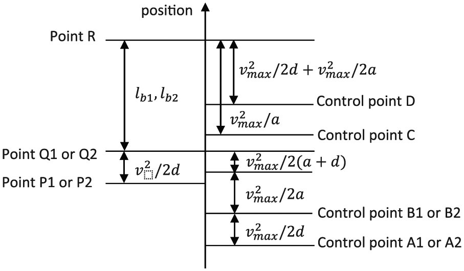
Control points set for the merging timing controller.

Table 8.

Conditions and decisions for the merging timing control.

Condition			Decision
The target AGV	The front AGV	v	u
The AGV arrives at control point A1 or A2	The front AGV is in the section farther than point D	$v < v_{\max}$	$u = a$
	The front AGV is in the section farther than point D	$v = v_{\max}$	$u = 0$
	The front AGV is in the section between point D and point A1 or A2	$v > 0$	$u = - d$
		$v = 0$	$u = 0$
The AGV exists in the sectionbetween point A1 or A2 and control point B1 or B2	The front AGV is in the section father than point C	$v < v_{\max}$	$u = a$
	The front AGV is in the section father than point C	$v = v_{\max}$	$u = 0$
	The front AGV is in the section between point B1 or B2 and point C	$v > 0$	$u = - d$
		$v = 0$	$u = 0$

AGV: automated guided vehicle.

Simulation results

The headway distance at the target merging point is controlled such that it is equal to or more than 2.337 m with the merging timing controller in this simulation. This is the border in Case 2-2(I) and Case 2-2(II) in section “Traffic jam analysis.” Simulation results are plotted in Figure 22. Figure 22 shows the traffic flow at the merging point for each AGV. The traffic flow with the merging timing control is better than the flow without the control. This is an effect due to the merging timing control. The optimal number of AGVs was 24 for these simulation conditions. The maximum traffic flow, 1444.7 1/h, with the merging control nearly achieved the theoretical maximum traffic flow of 1487.0 1/h. Table 9 shows a five-number summary of headway distance without timing control, whereas Table 10 shows the same with timing control. The headway distance of AGVs should be ≥2.337 with timing control. We found that it is almost achieved from Table 10 when the timing controller is used. The timing controller cannot exclude bad effects of traffic jams downstream of the merging point as mentioned in section “Merging timing control.” When the number of AGVs is ≥20, small traffic jams downstream of the merging point occurred. Thus, there were a few data, the headway distance of which was less than 2.337 m. The minimum headway distances without control are smaller than those with the control, but the traffic flows are almost the same in both cases when the number of AGVs is less than 20. The number of AGVs is not large enough to form traffic jams or a bottleneck at the target merging point. Thus, these cases are not the target of this study. And these are not applicable to Case 2-1 in section “AGV model behavior development around a merging point” because only two AGVs approach the blocking area once in Case 2-1, whereas more than two AGVs approach the blocking area multiple times in the cases above in this simulation. When the AGV density is low, a delay because of short headway distance does not negatively affect AGVs running far upstream. Thus, the total number of AGVs passing through the blocking area in 1 h is the same for the cases with the control and without the control. Figure 23 shows a point in the simulation with the timing control and Figure 24 shows a point in the simulation without the timing control. The AGV headway distance (red rectangle) in Figure 23 is larger than that in Figure 24. If the number of AGVs is fewer than 24, the simulations do not achieve the maximum traffic flow because the AGV density is low. If there are more than 24 AGVs, the AGVs are unable to move due to a heavy traffic jam, known as “deadlock.”

Figure 22.

The effects of the merging control based on the model.

Table 9.

Five-number summary of headway distance without timing control.

Number of AGVs	2	4	6	8	10	12	14	16	18	20	22	24	26	28	30
Maximum (m)	42.661	32.381	25.553	21.767	19.538	18.173	16.919	12.947	9.488	7.846	8.094	7.750	7.750	7.750	7.750
Upper quartile (m)	25.274	14.541	9.261	7.076	5.828	4.553	3.246	2.038	1.461	1.338	0.356	0.250	0.250	0.250	0.250
Median (m)	16.942	8.165	6.043	4.057	2.846	2.000	1.438	1.262	0.533	0.250	0.250	0.250	0.250	0.250	0.250
Lower quartile (m)	8.834	3.886	2.072	1.609	1.350	1.151	0.366	0.250	0.250	0.225	0.093	0.093	0.093	0.093	0.093
Minimum (m)	0.390	0.020	0.006	0.000	0.002	0.002	0.003	0.001	0.001	0.001	0.010	0.002	0.087	0.057	0.092
Ratio (%)of AGVs,the headwaydistances ofwhich are lessthan 2.337	5.727	16.170	27.007	35.904	45.412	56.541	67.058	77.148	86.232	94.548	99.009	99.869	95.506	99.105	95.556

AGV: automated guided vehicle.

Table 10.

Five-number summary of headway distance with timing control.

Number of AGVs	2	4	6	8	10	12	14	16	18	20	22	24	26	28	30
Maximum (m)	42.921	32.806	29.157	22.642	19.815	16.986	16.582	15.210	11.622	9.071	7.750	9.143	7.750	7.750	7.750
Upper quartile (m)	25.317	14.541	9.206	7.001	5.855	4.713	3.535	3.018	2.702	2.570	2.416	2.400	2.400	2.378	2.370
Median (m)	16.942	8.196	6.166	4.080	3.100	2.790	2.570	2.408	2.400	2.370	2.370	2.370	2.370	2.370	2.370
Lower quartile (m)	9.039	3.984	2.841	2.500	2.408	2.400	2.370	2.370	2.370	2.370	2.370	2.370	2.370	2.370	2.370
Minimum (m)	2.341	2.338	2.338	2.338	2.338	2.338	2.338	2.338	2.338	0.250	0.250	0.250	0.011	0.009	0.250
Ratio (%) of AGVs, theheadway distances of which are less than 2.337	0.000	0.000	0.000	0.000	0.000	0.000	0.000	0.000	0.000	0.185	1.508	1.979	8.085	6.311	6.452

AGV: automated guided vehicle.

Figure 23.

Simulation with the merging timing control.

Figure 24.

Simulation without the merging timing control.

This simulation forms a bottleneck at the target merging point. Thus, transfer flow is related to traffic flow, the relationship of which is shown in Figure 22. Transfer flow with a merging control is larger than that without a merging control, and traffic flows have the same trends as the transfer flows. This indicates that the merging timing control based on the developed model augments the traffic flow.

Conclusion

To achieve AGV and AMHS efficiency, there should be an optimal headway distance between AGVs. This study developed a mathematical model based on zipper merging for AGVs in an AMHS to achieve the optimal headway distance and maximum traffic flow. This model indicates that there is both an optimal headway distance and maximum traffic flow. We verified the model in part with fabrication using AutoMod simulations and, in another part, with actual AGV experiments. The results indicate that the mathematical model is feasible. Furthermore, we conducted a small full fabrication simulation, which indicated that a merging timing control, based on the model, augments AMHS transfer flow. We expect that macro-level⁹ and micro-level optimization (this study) will improve manufacturing techniques in real factories.

Footnotes

Handling Editor: Wu Naiqi

Declaration of conflicting interests

The author(s) declared no potential conflicts of interest with respect to the research, authorship, and/or publication of this article.

Funding

The author(s) received no financial support for the research, authorship, and/or publication of this article.

ORCID iD

Kenji Kumagai

References

Hayashi

Automated material handling system (AMHS) for semiconductor and LCD FAB. J Soc Mech Eng 2011; 114: 163–165 (in Japanese).

Han

Park

Chae

et al . Full fabrication simulation of 300 mm wafer focused on AMHS (automated material handling systems). In: Proceedings of the 3rd Asian simulation conference on systems modeling and simulation: theory and applications (AsiaSim 2004) (Lecture Notes in Computer Science) (ed DK

Baik

), Jeju City, South Korea, 4–6 October 2004, vol. 3398, pp.514–520. Heidelberg: Springer.

Tung

Sheen

Kao

et al . Optimization of AMHS design for a semiconductor foundry fab by using simulation modeling. In: Proceedings of the winter simulation conference (WSC), Washington, DC, 8–11 December 2013, pp.3829–3839. New York: IEEE.

Rank

Hammel

Schmidt

et al . Reducing simulation model complexity by using an adjustable base model for path-based automated material handling systems—a case study in the semiconductor industry. In: Proceedings of the winter simulation conference, Huntington Beach, CA, 6–9 December 2015. New York: IEEE.

Hoshino

Ota

Shizaki

et al . Comparison of an AGV transportation system by using the queuing network theory. In: International conference on intelligent robots and systems (IROS), Sendai, Japan, 28 September–2 October 2004, vol. 4, pp.3785–3790. New York: IEEE.

Govind

Roeder

Schruben

A simulation-based closed queueing network approximation of semiconductor automated material handling system. IEEE Tran Semiconduct Manuf 2011; 24: 5–13.

Zhou

System modeling and control with resource-oriented petri nets. 1st ed. Boca Raton, FL: CRC Press, 2009.

Cong

et al . Optimal petri net supervisors of discrete event systems via weighted and data inhibitor arcs. IEEE Access 2018; 6: 8245–8257.

Nakamura

Sawada

Shin

et al . Simultaneous optimization of dispatching and routing for OHT systems via state space representation. Trans Soc Inst Cont Eng 2014; 50: 210–218.

10.

Kumagai

Sawada

Shin

. Maximum throughput of automated guided vehicle system by use of models of traffic flow capacity and traffic flow consumption. In: SICE international symposium on control systems, Okayama, Japan, 8 March 2017. New York: IEEE.

11.

Sawada

Shin

Kumagai

et al . Optimal scheduling of automatic guided vehicle system via state space realization. Int J Automat Technol 2013; 7: 572–580.

12.

Verhaegh

Ploeg

Nunen

et al . Integrated trajectory control and collision avoidance for automated driving. In: Proceedings of the 5th IEEE international conference on models and technologies for intelligent transportation system (MT-ITS), Naples, 26–28 June 2017, pp.116–121. New York: IEEE.

13.

Hoshino

Tian

Komuro

et al . A model for merging section in transportation systems and its analysis. IEEJ Trans Ind Appl 2015; 135: 155–161 (in Japanese).

14.

Yanagisawa

Nishinari

Jutaigaku no cell automaton model. Bull Japan Soc Ind Appl Math 2012; 22(1): 2–14 (in Japanese).

15.

Nishi

Miki

Tomoeda

et al . Spontaneous zipper merging of self-driven particles. J Stat Mech Theory Exp 2011; 2011: P05027.

16.

Kumagai

Shin

Sawada

. Maximum traffic flow of automated guided vehicle based on jamology. In: Proceedings of the 19th international conference on mechatronics technology, Tokyo, Japan, 27–30 November 2015.

17.

Applied materials. Simulation AutoMod, http://www.appliedmaterials.com/ja/global-services/automation-software/automod/ (accessed 7 July 2018).

Maximizing traffic flow of automated guided vehicles based on Jamology and applications

Abstract

Keywords

Introduction

Traffic jam analysis

Problem definition

AGV specification

Specification of AGV behavior around blocking areas

Traffic flow comparison at a merging point

AGV model behavior development around a merging point

AGV model verification

Verification with simulation

Simulation conditions

Simulation results

Verification with actual AGVs

Experimental conditions

Experimental results

Effects of the merging control based on the model

Simulation conditions

Merging timing control

Simulation results

Conclusion

Footnotes

Declaration of conflicting interests

Funding

ORCID iD

References