
Abstract
The reliability optimization problem arises along with the increasing demands for products’ performance in practical engineering. Importance measures are capable of selecting critical components to gain the greatest improvement in system reliability with the constraint of maintenance cost. The characteristics of importance measure for four kinds of typical systems are discussed to illustrate the usage of importance measure in the practical reliability optimization. A reliability optimization model is eventually established and importance measure–based genetic algorithms are developed to solve the reliability optimization problem efficiently. Finally, two numerical experiments are implemented based on the smoke alarm systems. Experiment I is to illustrate the effectiveness of the importance measure–based genetic algorithms compared with standard genetic algorithm. Finally, the relationship between the order of component reliability improvement and the component parameters is analyzed in Experiment II.
Introduction
In reliability engineering, importance measures are generally used to identify the weakest components, and the system reliability can be improved through increasing the component reliability. The concept of importance measures is originally proposed by Birnbaum, 1 which stands for the contribution of component reliability changes to the system reliability. Some representative and latest importance measures include the uncertainty importance measure,2,3 the generalized Griffith importance measure, 4 and the integrated importance measure.5–8 With the importance values of all components, proper actions can be applied to the weakest component to improve system reliability. By now, importance measures have been widely used in practice to identify the weaknesses of different kinds of systems. Many importance measures have been proposed with respect to the diverse considerations of system performance, reflecting different probabilistic interpretations and potential applications. 9 Barker et al. 10 proposed the component importance measure for the network based on resilience. Baroud et al. 11 demonstrated a time-dependent paradigm for resilience and the associated stochastic metrics in a waterway transportation context, and deployed two stochastic resilience-based component importance measures. A novel probability density function estimation–based method is proposed to efficiently evaluate the moment-independent index. 12 Zhai et al. 13 presented a general formulation of the moment-independent importance measures in reliability and safety engineering. Lisnianski et al. 14 considered a reliability importance evaluation for components in an aging multi-state system to reduce the computational burden of solving the real-world problem. Shen and Cui 15 considered an importance measure calculation for the circular consecutive-k-out-of-n system with sparse d. Wu et al. 16 introduced an importance measure, called component maintenance priority, which is used to select components for preventive maintenance. Dui et al. 17 proposed a new importance measure for analyzing the impact of external factors on system performance. In view of the negative impact of functional dependency, Wang et al. 18 provided an alternative importance measure for measuring the importance of components in mechatronic systems. The variance-based global importance measure is used to evaluate the importance of a component to the mission reliability of phased mission systems while the reliabilities of all components vary randomly. 19
The reliability optimization problem involves minimizing the system cost subject to reliability requirement or maximizing the system reliability under resource constraints (such as cost, weight, or volume), which has been proved to be NP-hard. 20 Peng et al. 21 investigated the reliability analysis and optimal structure of series–parallel phased mission systems that maximizes the system reliability. Meng et al. 22 proposed an evidence-based collaborative reliability optimization method to handle epistemic uncertainties of complex engineering systems. Li et al. 23 put forward a hybrid reliability optimization method for various pallets with random parameters, which aimed to provide an effective computational tool for reliability design of the pallet system. Liu et al. 24 presented an approach of joint redundancy and imperfect maintenance strategy optimization for multi-state systems. Li et al. 25 proposed a two-stage approach by applying a multiple objective evolutionary algorithm for solving multi-objective system reliability optimization problems.
Heuristics methods, such as genetic algorithm (GA), have been widely applied for this type of problem owing to their effectiveness and robustness. Based on genetic evolutionary mechanism, GA has been applied to solve the multi-objective discrete reliability optimization problem in a k-dissimilar-unit non-repairable cold-standby redundancy system. 26 A modified non-dominated sorting GA is used to search the Pareto optimal solutions of the multi-objective multi-stage formulation for reliability growth planning. 27 The application of importance measures can direct the evolution and limit the randomness in heuristics algorithms by prioritizing the components with higher importance value for reliability improvement. Based on importance measures, heuristics have been developed to solve the component assignment problem in Lin/Con/k/n systems, where system reliability is maximized by optimally assigning interchangeable components to different positions.28–31
This article concentrates on estimating the reliability improvement of each component to maximize the system reliability under cost constraint. The remainder of this article is structured as follows. Section “Typical importance measures” introduces two traditional importance measures and the relationship between them. In section “Characteristics of importance measures for typical systems,” changes of component importance in typical systems are demonstrated to guide practical reliability optimization. Model of reliability optimization and the importance measure–based GAs are developed in section “Reliability optimization formulations.” In section “Case study,” some smoke alarm systems are introduced to illustrate the effectiveness of importance measure–based GAs and the relationship between the order of component reliability improvement and component parameters is also analyzed. Section “Conclusion” summarizes this work.
Typical importance measures
The typical importance measures such as Birnbaum importance measure (BM) and the Δ-importance measure (DM) are introduced in this section.
BM
The BM is used to evaluate the significance of a component to system reliability
1
and is the effect of the changes of component reliability on the system reliability. The BM of component i in a system is defined in equation (1), where

DM
The DM
32
is developed to evaluate the increment of the system reliability due to the improvement of the component reliability. And
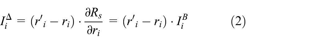
From equation (2), it is clear that DM is the BM times the component reliability improvement. The BM actually is taking the partial derivative of the system structural function with respect to component reliability, but the DM also needs to consider the component reliability improvement.
Characteristics of importance measures for typical systems
Importance measures are used to evaluate the importance of various components in a system. The importance measure value may not be as useful as their relative ranking. Characteristics of importance measure for components in typical systems, which include series, parallel, series–parallel, and parallel–series systems, are of great significance to guide the practical optimization procedure. The changes of BM and DM with the increase in the objective component reliability are discussed as follows.
Series system
According to the calculation of BM in the series system, the lower a component’s reliability is, the larger the BM of the component is. But DM should consider the component reliability improvement and BM. The component with the largest importance is regarded as the objective component, and assume component 1 as the objective component to analyze the changes of BM and DM. As the reliability of the objective component increases, BM and DM of the remaining components also increase (Figure 1). In Figure 1, the bold up arrow represents the changes of objective component reliability, and the other arrows represent the changes of BM for the corresponding components. DM of the objective component is increasing with the increase in objective component reliability, but BM of the objective component is unchanging. If the importance of another component is larger than that of the original objective component, then it is defined as the new objective component. This iteration is a better way to improve the system reliability in the actual optimization problems.

Changes of BM and DM with the increasing reliability of objective component 1 in the series system.
Parallel system
In a parallel system, the higher a component’s reliability is, the larger the BM of the component is. But DM should consider the component reliability improvement and BM. As the reliability of the objective component increases, BM and DM of the remaining components decrease instead (Figure 2). DM of the objective component is increasing with the increase in objective component reliability, but BM of the objective component is unchanging. In order to obtain the maximum system reliability effectively, the reliability of component 1 needs to improve its reliability as much as possible. If the system reliability cannot satisfy the reliability constraint, the component with the largest importance measure after the improvement should be considered as the new objective component to improve its reliability.

Changes of BM and DM with the increasing reliability of objective component 1 in the parallel system.
Series–parallel system
A series–parallel system is a series of parallel systems. The lower a subsystem’s reliability is, the larger the BM of the subsystem is. The subsystem with the largest importance measure is defined as the objective subsystem, and the component with the highest importance measure in the subsystem is regarded as the objective component. For the series–parallel system, assume that component 1 in the left first subsystem is the objective component. As the reliability of the objective component increases, BM and DM of components in series with the objective subsystem increase, but those of components in parallel with the objective component decrease instead, as shown in Figure 3. DM of the objective component is increasing with the increase in objective component reliability, but BM of the objective component is unchanging. In Figure 3, the objective subsystem is the left first subsystem and the objective component is component 1 in this subsystem.
Changes of BM and DM with the increasing reliability of objective component 1 in the series–parallel system.
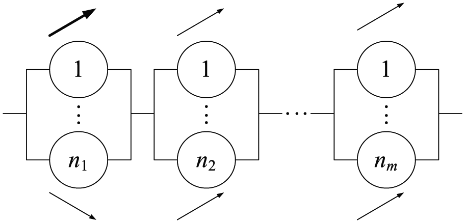
Parallel–series system
A parallel–series system is the parallel of series systems. The higher a subsystem’s reliability is, the larger the BM of the subsystem is. The subsystem with the highest importance measure is defined as the objective subsystem, and the component with the highest importance measure in the subsystem is the objective component. In Figure 4, as the reliability of component 1 in the top subsystem increases, BM and DM of components in the other parallel subsystems decrease, but those of components, which are in series with component 1 in the top subsystem, increase. However, DM of the objective component is increasing with the increase in objective component reliability, but BM of the objective component is unchanging.

Changes of BM and DM with the increasing reliability of objective component 1 in the parallel–series system.
Reliability optimization formulations
Assumptions of the reliability optimization problem
The reliability optimization problem under study belongs to the reliability allocation category, which is proved to be NP-hard and noted as Problem P1. 33 With the limitation of total cost, the objective of Problem P1 is to maximize system reliability by increasing the reliability of individual components. The assumptions of the reliability optimization problem studied in this article are shown as follows:
The system is coherent and monotonous;
Components are statistically independent;
System and components only have two disjoint states, namely, failed and operational;
The overall cost is the summation of individual component costs.
Cost function
Mettas
34
established the relationship among component reliability, feasibility of reliability improvement, and cost. If the component reliability is known, the cost can be calculated based on the maximum achievable reliability and the minimum acceptable reliability of the component. The cost of component i with reliability
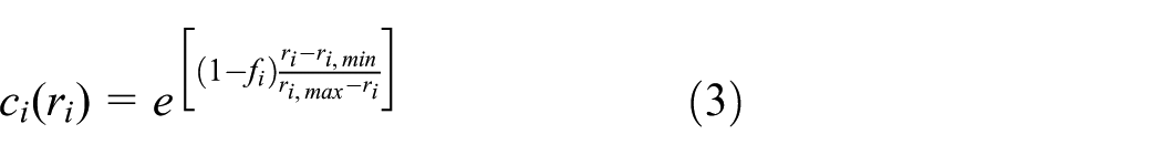
Note that this penalty function acts as a weighting factor that captures the difficulty of increasing the component reliability from
Therefore, the cost of component from

where
Reliability optimization model
Subject to overall cost constraint
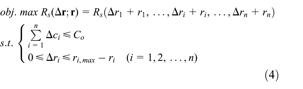
For the reliability optimization model, the objective function is to maximize the system reliability, and the decision variable is the improvement of each component reliability, which is noted as
Mechanism of applying importance measure
When the reliabilities of n components can be improved, the question is how to appropriately determine the reliability improvement of each component to maximize the system reliability with the constraints of overall cost. BM can be used to express the improvement of system reliability if the component reliability is increasing.
Suppose that a system consists of n components.
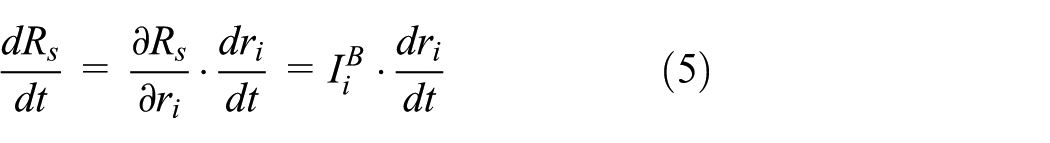
From equation (5), if the reliability increment of component i is determined, the larger the

As shown in equation (6), with the same reliability increment, the component with the highest BM can bring the highest improvement of system reliability. If the increment of all components is not the same, the component with the highest DM can bring the highest improvement of system reliability. Therefore, the component with larger BM or DM should be given more priority for reliability improvement.
Algorithms for the reliability optimization model
Since Problem P1 is a non-linear, non-convex optimization model, heuristic algorithms, such as GA, have been widely applied to solve this type of problem. Based on the advantages of importance measure, the importance measure–based GA is developed to solve Problem P1 by taking into account the variability of reliability limits and overall cost constraint. In these algorithms, local search is executed based on BM and DM. The flowchart of the importance measure–based GA is shown in Figure 5, and its detailed procedure is as follows:
Step 1. Confirm the objective function and solution space
The objective function is the system reliability after improvement, and the solution space is a set of the reliability increment of n components, which can be recorded as
Step 2. Confirm the encoding and decoding method
We use the real number encoding method to represent the reliability increment, where a gene is the real value of the component reliability increment, and all the n genes are treated as a chromosome. Because the gene is the real value of reliability increment, the decoding method need not be used in this algorithm.
Step 3. Initialize the population
According to the population size, s chromosomes are generated based on the solution space, and each chromosome is the potential solution of the problem, which has n positions recording the increment of n components’ reliability.
Step 4. Calculate the fitness of each chromosome and identify the best chromosome
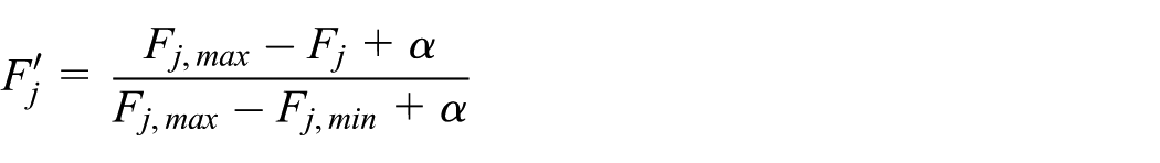
Considering the improvement cost, if the cost is higher than the overall cost constraint, the fitness will be modified with the penalty. Therefore, the fitness function is viewed as
Step 5. Inspect whether the termination condition is satisfied
If the algorithm reaches the maximum iteration M, the algorithm will be terminated and output the solution. Generally, the value of M is suggested to vary in the range of [100, 1000].
Step 6. Perform selection on current population
According to the roulette strategy, the offspring population is generated through selecting s chromosomes from the current population. For selecting appropriate chromosomes with the higher system reliability and the constraints of overall cost, the normalization is conducted to modify the fitness of each chromosome by
where
Step 7. Perform crossover on population
Generate a random number between 0 and 1; if the number is less than
Step 8. Perform mutation on population
Mutation is performed on all chromosomes to maintain the diversity of the population with a probability of
Step 9. Perform local search based on importance measure
According to section “Mechanism of applying importance measure,” the components with larger importance measure should be given priority for the reliability improvement during the optimization process. Local search based on importance measure is introduced to give the optimization direction. The importance measure of each gene is calculated; the gene with the maximum importance measure will be replaced with a random number
Step 10. Perform the elitism strategy and generate the new offspring population
The chromosome with the worst fitness should be replaced with the best chromosome saved in Step 4. This process makes the offspring in the current population not worse than that in the previous population.
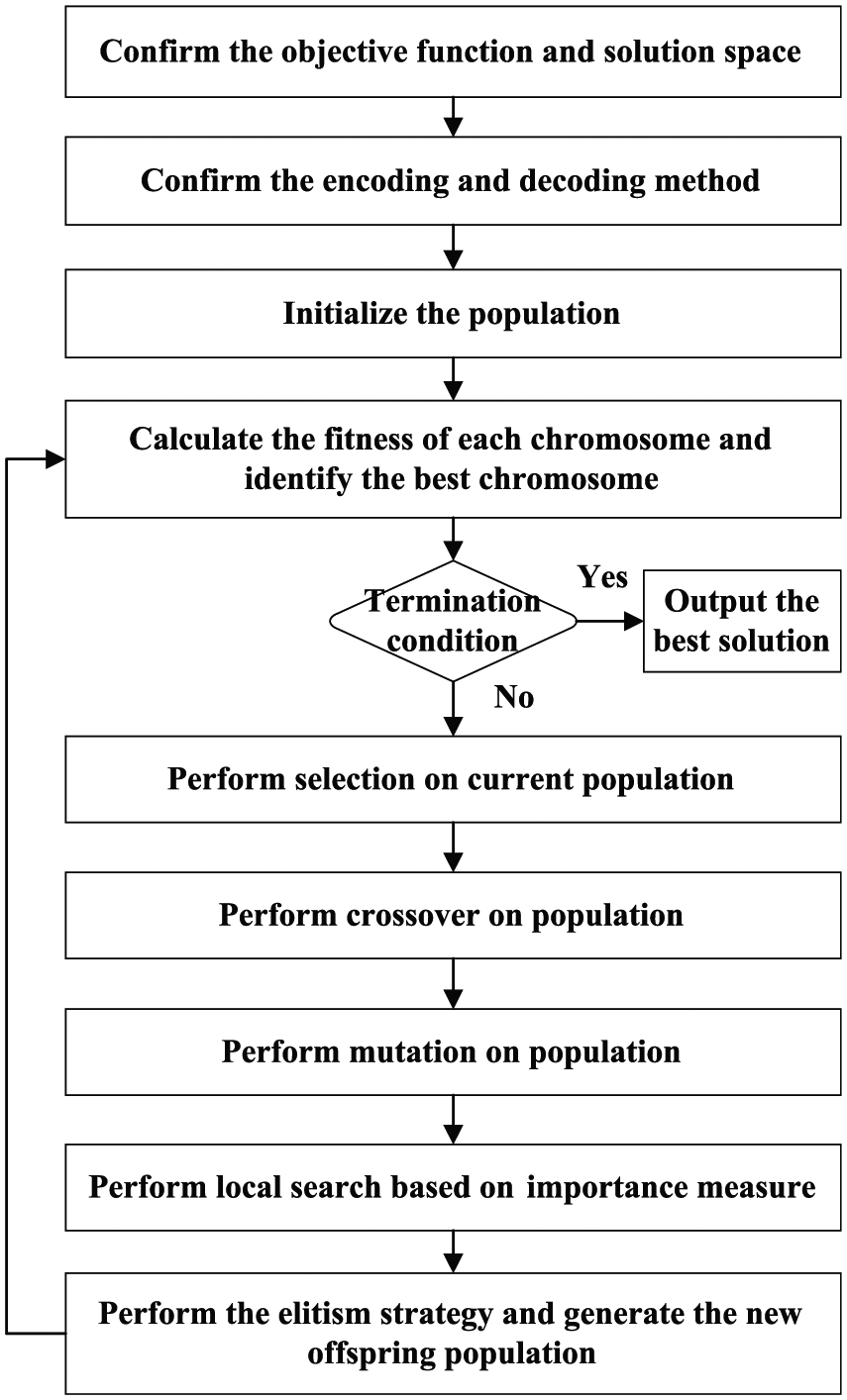
The flowchart of the importance measure–based genetic algorithm.
In this article, the Birnbaum importance measure–based genetic algorithm (BGA) and Δ-importance measure–based genetic algorithm (DGA) are introduced to solve the optimization problem. The procedures of BGA and DGA are the same as the importance measure–based GAs except for Step 9. The differences of BGA and DGA focus on the local search process, and the other processes of these two algorithms are all the same. For DGA, the importance measure in Step 7 should be replaced by the DM, which is the local search based on DM to find the optimal solution. For the BGA, the importance measure in Step 9 should be replaced by BM. The difference of BGA and DGA is in whether the local search considers the improvement of component reliability in the importance measure or not.
Case study
The smoke alarm systems are the typical mixed system, which includes monitors, sensors, logical processors, and controlling elements. The monitor is used to monitor the states of components in the system; the sensors are used to detect the smoke density and collect the smoke data; the logical processers are used to deal with the collected data; the controlling elements are used to trigger the alarms in the system.
In order to improve the system reliability, a company selects a kind of alarm system which is an integration of two sets of smoke alarm systems from different distributors. Therefore, the smoke alarm system from the first distributor is noted as Case I, the smoke alarm system from the second distributor is noted as Case II, and the smoke alarm system that the company is using is noted as Case III. The structures of these three cases are shown in Figure 6. Case I is a typical series–parallel system, which has two sensors and two controlling elements. Case II is a simple mixed system because sensors 4 and 5 are connected in series. Case III actually is the integration of Cases I and II, which is a complex mixed system.
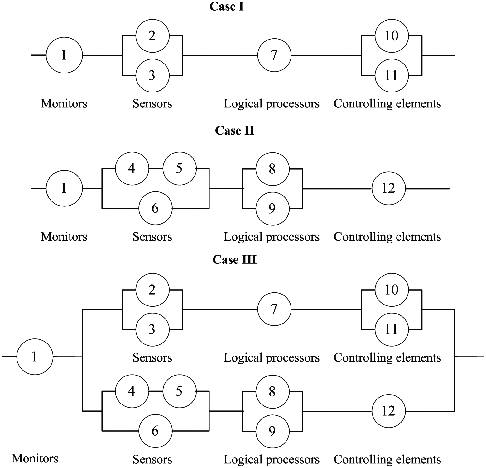
The smoke alarm system structure of the three cases.
The improvement cost varies depending on the component type, including feasibility, minimum reliability, maximum reliability, and current reliability. Data of the components are shown in Table 1.
Parameters of each component.

Design of experiments
In order to demonstrate that BGA and DGA are better than GA, the first experiment is designed through comparing the solutions of GA, BGA, and DGA. The second experiment is presented to determine the order of component reliability improvement to obtain the optimal solution.
Experiment I. The parameters in the three algorithms are the same, with
Experiment II. For each case, select five instances C4, C8, C12, C16, and C20 and choose the optimal solution of DGA from the 100 trials randomly. The relationship of improvement order of components with component parameters is analyzed.
Results of Experiment I
GA is a kind of random algorithm, and the mean optimal results and the robustness of the results are two important factors of the effectiveness of algorithm. Therefore, the results of the experiment mainly consider the mean system reliability and the robustness of the three algorithms for different cases.
Comparisons of the mean optimal solutions
Mean system reliability of Case I
For 20 instances in Case I, the mean system reliability after improvement and the mean number of generations to obtain the solutions obtained by GA, BGA, and DGA are shown in Table 2.
The mean system reliability and the mean number of generations for Case I.

GA: genetic algorithm; BGA: Birnbaum importance measure–based genetic algorithm; DGA: Δ-importance measure–based genetic algorithm.Note: The bold values signifies that the best mean value of system reliability and convergence generation obtained by three algorithms for Case 1.
From Table 2, we can find that the mean system reliability values of BGA and DGA are both larger than that of GA for 20 instances. And the mean convergence generation values of BGA and DGA are always less than that of GA except for instance C2. In order to compare the effectiveness of BGA and DGA, we can find that it is more possible to obtain better solution with DGA because we can find that there are more instances that the mean system reliability of DGA is larger than that of BGA, which is shown in Figure 7. In terms of mean system reliability, BGA obtained the highest reliability in 5 of 20 cases and DGA obtained the highest reliability in 15 of 20 cases. In terms of the mean number of generations to obtain the near-optimal solution, BGA obtained the fewest number of mean convergence generations in 11 of 20 cases and DGA obtained the fewest number of generations in 8 of 20 cases. However, the mean convergence generation of DGA is near to that of BGA, with the difference being less than 10.
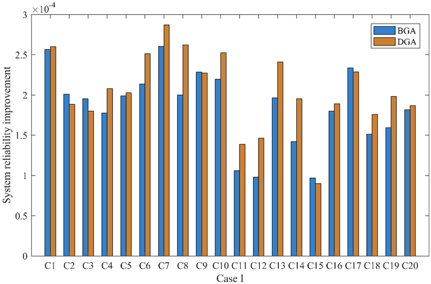
Comparison of the mean system reliability for Case I.
Mean system reliability of Case II
For 20 instances in Case II, the mean system reliability after improvement and the mean number of generations to obtain the solutions runs by GA, BGA, and DGA are shown in Table 3.
The mean system reliability and the mean number of generations for Case II.
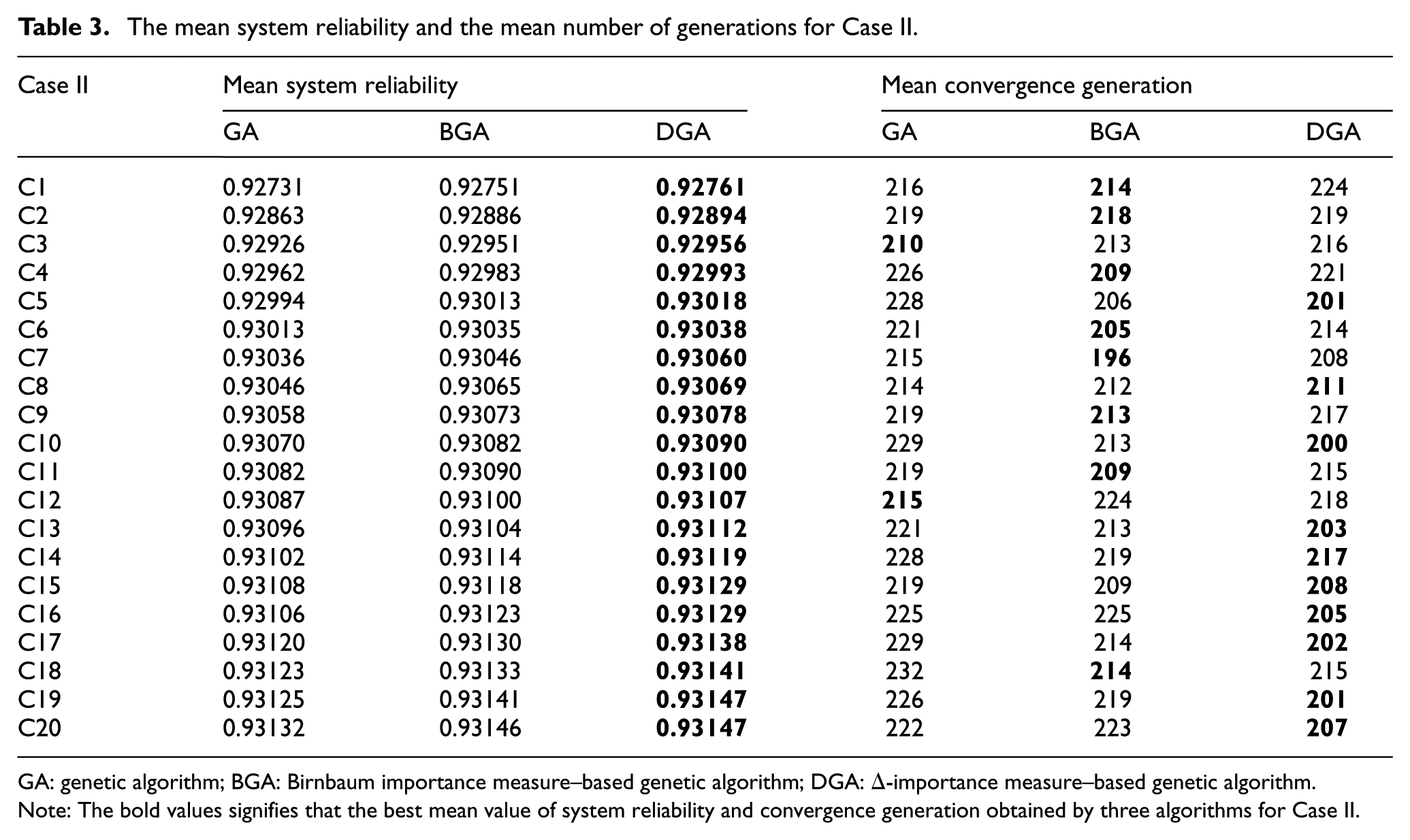
GA: genetic algorithm; BGA: Birnbaum importance measure–based genetic algorithm; DGA: Δ-importance measure–based genetic algorithm.Note: The bold values signifies that the best mean value of system reliability and convergence generation obtained by three algorithms for Case II.
From Table 3, we can find that the mean system reliability values of BGA and DGA are both larger than that of GA for 20 instances. And the mean convergence generation values of BGA and DGA are almost less than that of GA except for instances C2 and C12. In order to compare the effectiveness of BGA and DGA, we can find that DGA can obtain the better solution than BGA because we can find that the mean system reliability of DGA is larger than that of BGA for all 20 instances, which is shown in Figure 8. In terms of mean system reliability, BGA obtained the highest reliability in none of 20 cases and DGA obtained the highest reliability in all the 20 cases. In terms of the mean number of generations to obtain the near-optimal solution, BGA obtained the fewest number of mean convergence generations in 7 of 20 cases and DGA obtained the fewest number of generations in 11 of 20 cases.

Comparison of the mean system reliability for Case II.
Mean system reliability of Case III
For 20 instances in Case III, the mean system reliability after improvement and the mean number of generations to obtain the solutions runs by GA, BGA, and DGA are shown in Table 4.
The mean system reliability and the mean number of generations for Case III.
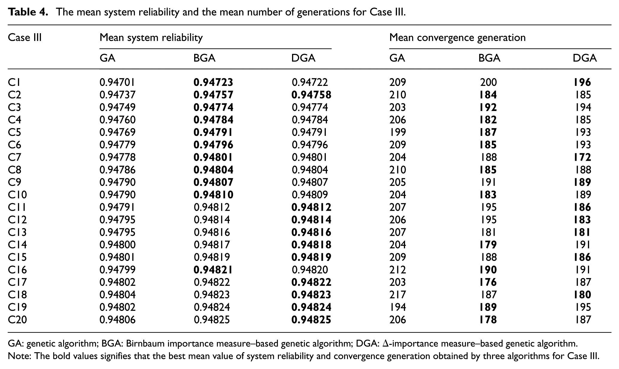
GA: genetic algorithm; BGA: Birnbaum importance measure–based genetic algorithm; DGA: Δ-importance measure–based genetic algorithm.Note: The bold values signifies that the best mean value of system reliability and convergence generation obtained by three algorithms for Case III.
From Table 4, we can find that the mean system reliability values of BGA and DGA are both larger than that of GA for 20 instances. And the mean convergence generation values of BGA and DGA are less than that of GA. In order to compare the effectiveness of BGA and DGA, we can find that the mean system reliability of DGA is almost the same as that of BGA, which is shown in Figure 9. In terms of mean system reliability, BGA obtained the highest reliability in 11 of 20 cases and DGA obtained the highest reliability in 9 of 20 cases. In terms of the mean convergence generations to obtain the near-optimal solution, BGA obtained the fewest number of mean convergence generations in 12 of 20 cases and DGA obtained the fewest number of generations in 8 of 20 cases. We can also find that BGA is better to solve the instances with the lower cost constraints (instances 1–10) and DGA is better to solve the instances with higher cost constraints (instances 11–20).

Comparison of the mean system reliability for Case III.
Comparisons of the robustness
The coefficient of variation (CV) is applied to evaluate the robustness of the three algorithms, which is presented in Table 5. The calculation formula of CV is as follows
Comparisons of the three algorithms in terms of coefficient of variation.
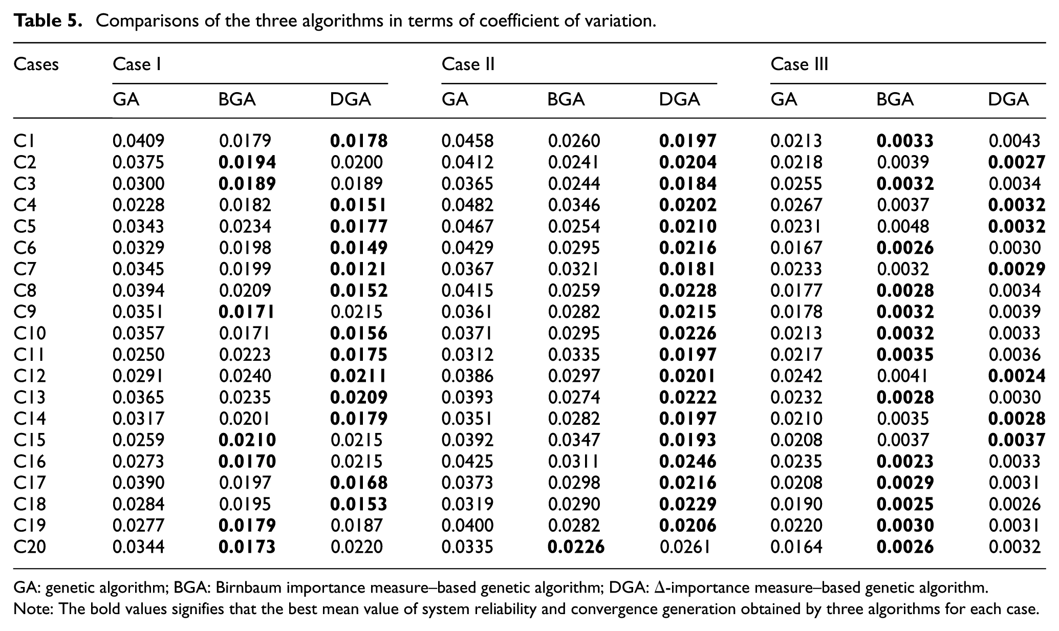
GA: genetic algorithm; BGA: Birnbaum importance measure–based genetic algorithm; DGA: Δ-importance measure–based genetic algorithm.Note: The bold values signifies that the best mean value of system reliability and convergence generation obtained by three algorithms for each case.
As shown in Table 5, the CV is very low for the three methods, which indicates that the robustness of GA, BGA, and DGA are all pretty good. For Case I and Case II, the CV of DGA is very likely less than that of BGA and GA. For Case I, BGA obtained the lowest CV in 7 of 20 cases and DGA obtained the lowest CV in 13 of 20 cases. For Case II, BGA obtained the lowest CV in 1 of 20 cases and DGA obtained the lowest CV in 19 of 20 cases. For Case III, the CV for BGA seems better than that of DGA, but the value is almost the same as that of DGA.
For the results of Experiment I, the effectiveness of BGA and DGA is better than that of GA, that is to say the local search based on the importance measure can obtain the better solution. DGA can solve Cases I and II more effectively, especially for Case II. For Case III, although the BGA performs better than DGA, the solution is almost the same. Therefore, the DGA is better to solve this optimization problem P1 than BGA.
Results of Experiment II
According to the results of Experiment I, the solution of DGA is selected to discuss the relationship of the improvement order of components with component parameters. The solution of instances C4, C8, C12, C16, and C20 for the three cases is selected randomly from the experiments, which is generated by DGA. The optimal solution of the cases based on DGA is shown in Table 6.
Optimal solution of cases based on DGA.

DGA: Δ-importance measure–based genetic algorithm.
In order to analyze which component should be selected first to improve its reliability to maximize the system reliability, the improvement percentage of each component i is introduced to evaluate the utilization of component reliability improvement. The calculation of improvement percentage for component i can be obtained by equation (8). The improvement percentage of each component is shown in Table 7

Improvement percentage of each component for the selected instances.
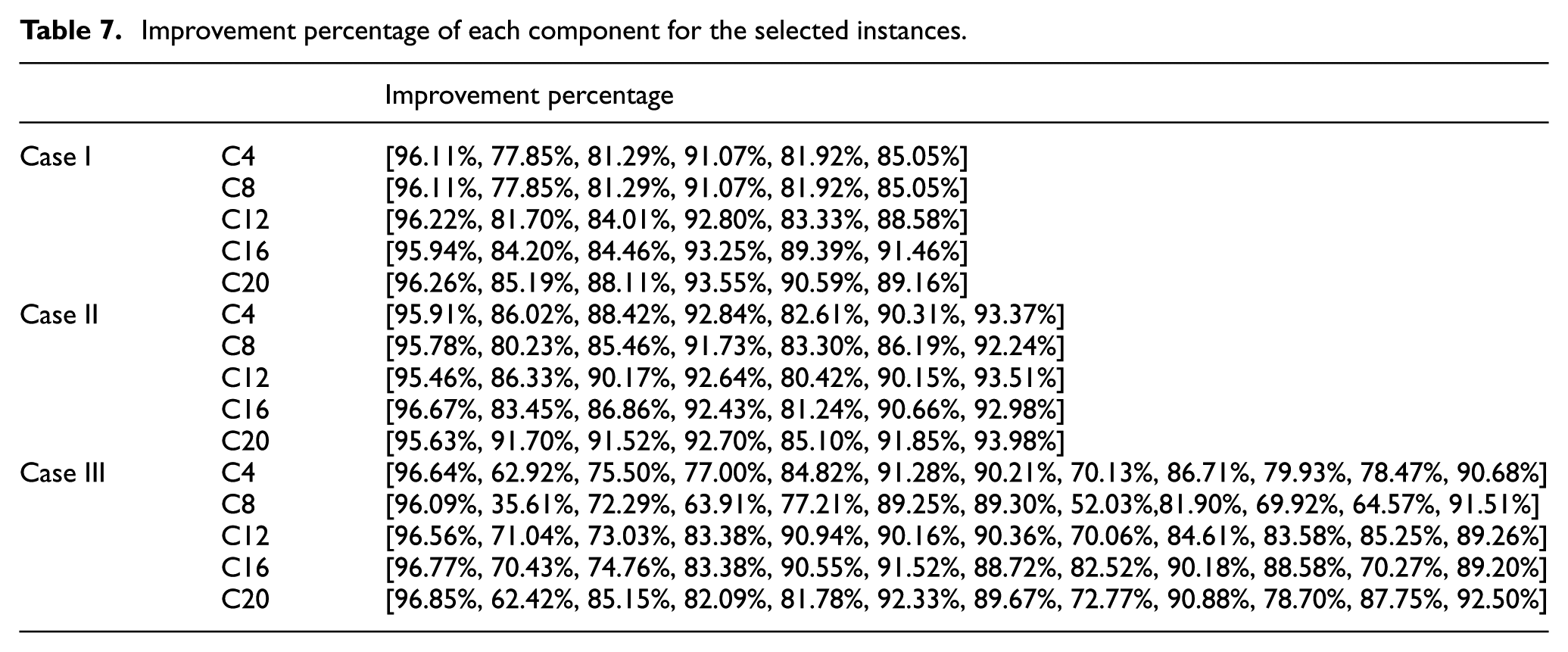
When the reliability of component i is near to the
From the improvement percentage, we can obtain the general order of component reliability improvement. In order to build the relationship of the improvement order of components with component parameters, the greedy strategy is easy to determine and we need to improve the component reliability with the lower unit cost. The improvement of system reliability with unit cost

Based on the component parameters, we can obtain the improvement of system reliability with unit cost for each component as shown in Table 8.
Improvement of system reliability with unit cost of each component for the three cases.

From Table 8, we can find the order of component reliability improvement for the three cases, and the order is consistent with the analysis of the solution. For Case I, the improvement order is 1-7-11-10-3-2; for Case II, the improvement order is 12-1-9-5-6-4-8; for Case III, the improvement order is 1-12-7-6-9-11-10-5-8-3-4-2. Therefore, the order of component reliability improvement can be determined based on
Conclusion
In this article, BM and DM are introduced into the GA for solving the reliability optimization problem with component improvement cost effectively. Numerical experiments are implemented to evaluate and justify the effectiveness of the importance measure–based GAs based on the smoke alarm systems. The results of Experiment I show that BGA and DGA perform better than GA, which can reach the near global solution in a more effective way, and DGA is better than BGA in general. The results of Experiment II show that the order of component reliability improvement can be determined by the system reliability improvement with unit cost, which is related with the component parameters and importance measure. The future work will focus on the applications of importance measure for more practical complex systems such as the reconfigurable systems or the phased mission systems.
Footnotes
Handling Editor: Xihui Liang
Declaration of conflicting interests
The author(s) declared no potential conflicts of interest with respect to the research, authorship, and/or publication of this article.
Funding
The author(s) disclosed receipt of the following financial support for the research, authorship, and/or publication of this article: This work was supported by the National Natural Science Foundation of China (No. 71401016) and the Fundamental Research Funds for Central Universities of Chang’an University (Nos 300102228110 and 300102228402).