
Abstract
This article describes a model-free adaptive control method for knee joint exoskeleton, which avoids the complexity of human–exoskeleton modeling. An important feature of the proposed controller is that it uses the input and output data of the knee joint angle to control the exoskeleton. Furthermore, discrete sliding mode control law and prior torque are introduced to improve the accuracy and robustness of the system. Prior torque of knee joint is obtained through the walking simulation of human–exoskeleton modeling. Specially, the experiment is carried out by using the co-simulation automatic dynamic analysis of mechanical systems and MATLAB. Data from these assessments indicate that the proposed strategy enables the knee exoskeleton to track the trajectory of angle well and has a good performance on walking assistance.
Keywords
Introduction
Exoskeleton equipment is an electromechanical device used to enhance, help and restore the body’s athletic ability. The design and development of exoskeleton is one of the hotspots of scholars. A variety of exoskeletons1–4 have been developed. The Berkeley Lower Extremity Exoskeleton (BLEEX) developed by Berkeley University of California is the first type of exoskeleton that can carry loads and walk autonomously with a power source. The hybrid assistant limb (HAL) of University of Tsukuba in Japan is an enhanced exoskeleton based on electromyography (EMG) signals to detect human intentions for control; Lokomat developed by Hocoma Company of Switzerland is a rehabilitative exoskeleton for indoor walking training.
The knee exoskeleton is a branch of lower limb exoskeletons. Due to the aggravation of aging and the fragile characteristic of the knee joint, the demand for knee exoskeleton is increasing. Some active researches have been conducted.5,6 Pratt et al. 7 presented a one-degree-of-freedom exoskeleton called the RoboKnee and used proportional amplification control to assist the human locomotion. Fleischer and Hommel 8 developed the TUPLEE exoskeleton, which is driven by a biomechanical model that evaluates the EMG signals of the operator to derive the desired torque. The control system of TUPLEE acts as a torque amplifier and the limitation of the control method is that the EMG signals are easily affected by muscle fatigue factors and the placement of different electrodes. Rifaï et al. 9 established the dynamics of shank-foot-exoskeleton system based on the Lagrangian method and presented a bounded control strategy of a knee joint exoskeleton. Chen et al. 10 proposed an iterative prediction-compensation motion control scheme for an exoskeleton knee joint. A focused time-delay neural network and force–position control paradigm are used to control the motion of the knee joint, but the control calculations have higher requirements and the neural network requires multiple trainings. Han et al. 11 designed a multi-modal elastic actuator based on the movement mechanism of lower limb muscles during walking. The dynamic modeling of the actuator is carried out and the control strategy based on the motion state machine is used to control. In addition, Han et al. 12 established the human–machine dynamic model and presented an emulated inertia compensation control method based on admittance principle to solve the operator’s motion tracking problem.
The above control methods are mainly based on accurate dynamic models. However, the structure of the human–robot system is hard to determine and the parameters are difficult to identify, which makes the model error inevitable in modeling. Some model-free control methods received increasing attention. Time-delay estimation (TDE) is an online system dynamics estimation method which estimates the unknown dynamics of the plants using the time-delayed information of systems. The TDE technique causes the errors because the estimation is delayed by one sampling step. Han et al. 13 designed the intelligent proportional–integral (PI) controller and adaptive nonsingular fast terminal sliding mode control to suppress such TDE errors. Wang et al. 14 proposed a fractional-order nonsingular terminal sliding mode method based on TDE to stabilize system error to zero in finite time. Repetitive learning control (RLC) is used to deal with repetitive control tasks with periodic uncertainties, and human normal walking shows repetitive features in general. Yang et al. 15 designed a RLC to fulfill the designated tracking task for the lower limb exoskeleton under the framework of backstepping design. Model-free adaptive control (MFAC), as a data-driven control method, is introduced in this article. The distinct feature of the approach is that the controller was designed based on the input and output data of the plant. The MFAC method is different from TDE. The TDE approach usually constitutes the baseline part of the control algorithm to estimate the uncertainties of the model, and other control methods need to be adopted to suppress the TDE errors and improve the control precision. The MFAC method adopts a novel dynamic linearization method and introduces pseudo-gradient (PG) concept for the discrete-time nonlinear system. Instead of identifying the complex nonlinear model system, an equivalent dynamical linearization model is established. Based on the dynamic linearization method, the values at discrete-time points of complex systems are transformed into time-varying linearized data in incremental form. MFAC can be used as an independent controller method or combined with other methods to improve control performance. The approach has been successfully implemented in many practical applications, for example, chemical distillation tower, communication topology tracking, parking system, and small unmanned helicopter control.16–19
The main contribution of this work is the development of control approaches of knee joint exoskeleton for assistance. Based on the input and output data of the system, MFAC approach combined with discrete sliding mode and prior torque is designed. Discrete sliding mode control is characterized by fast response, insensitivity to disturbances, and parameters’ perturbation, and meanwhile, it can be applied to nonlinear systems. The introduction of discrete sliding mode control law can enhance the robustness of the system. The key of the control is that the output of knee joint torque can track the gait changes of the lower limbs well. The prior torque of knee joint during normal walking is obtained by simulation, and the anti-interference capability of the control system is improved by using data trend of prior torque.
Dynamic model and transformation of lower extremity exoskeleton
The lower extremity and exoskeleton model is shown in Figure 1. Based on the Lagrange dynamics method, the general dynamics of the lower extremity system can be written as follows

where

Human lower limb and exoskeleton model.
Equation (1) can be deduced to

In this article,
For a discrete-time system,

When the sampling time of the discrete-time system is sufficiently small, the sampling time is set to T, and


Substituting

Equation (6) satisfies the following assumptions.
Assumption 1
The partial derivatives of equation (6) with respect to control input
Assumption 2
System (6) is generalized Lipschitz,
20
that is, for any k and

where b is a positive constant. In order to describe easily, the output changes and input changes at two adjacent moments are defined as


For a system that satisfies two assumptions with

The proof of equation (9) is detailed in Appendix 1.
Controller design
Block diagram of the controller is shown in Figure 2. The controller includes three parts: MFAC, discrete sliding mode control, and prior torque.
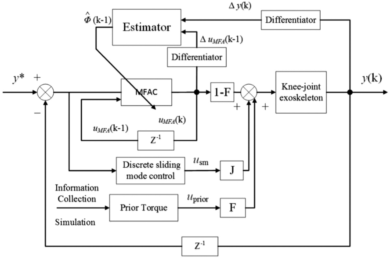
Control block diagram of knee joint exoskeleton (J represents the weight factor of discrete sliding mode control and J is positive constant; F represents the weights assigned to knee prior torque input
MFAC
In order to prevent the control algorithm from generating steady-state tracking error and excessive control input, the following control input criterion function 22 is used to design the controller
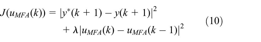
where

where

where

where
Discrete sliding mode control law
The procedure of sliding mode control consists of two steps, where we select the sliding surface at first and then design the control law. The sliding surface for knee joint is selected as

where C is the sliding surface parameter which is to ensure the gradual stability and fast response speed of sliding mode motion.


Equation (17) is the introduced discrete exponent reaching law, where T is the discrete sampling time,

In order to reduce the jitter in sliding mode control, the saturation function
Substituting equations (7), (9), (15) and (16) into equation (17), the sliding mode control input

Prior torque
In order to obtain the prior torque of the knee joint, the joint angles of human lower extremities are collected first, and then, the angle data are used to drive the exoskeleton model of the lower extremities in the ADAMS software to obtain the simulated knee joint prior torque.
The VICON gait analysis system is used in the data collection of the lower extremities. As depicted in Figure 3, markers are located on the left and right sides of the body’s hip joint, thigh, knee joint, shank, ankle, and heel. The trajectory of the infrared reflective markers is captured by infrared cameras in the VICON three-dimensional gait analysis system. The system can obtain the trajectory of each marker when the human body moves and the angle data of each joint of the lower extremity can be obtained through data processing. A 25-year-old female subject with the height of 175 mm and weight of 62 kg volunteered to participate in the test. The subjects were tested without load and walked at a normal speed of 1.3 m/s. The experimental protocol was approved by the Institutional Review Board of Hebei University of Technology. The subject provided informed consent for the experiment.

Location of markers.
We analyze the knee joint angle data collected and find that the range of knee joint angle in the gait cycle is 6.71°–65.11°. Usually, the knee angle can be straight from 0° to 155° depending on the thickness or tightness of the tissue under joint of the individual. The minimum angle of knee joint must not be negative, otherwise it will seriously damage the knee joint.
The joint angle data collected are imported into ADAMS software, and the human body model is driven by the CUBSPL function. Figure 4 shows the knee torque viewed in the post-processing module after the simulation.
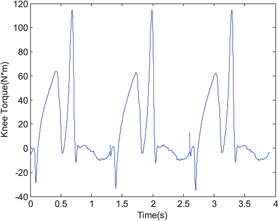
Simulation torque of knee joint.
The controller makes use of the data trend of the prior torque to improve the anti-interference ability of the control system. In order to avoid the excessive influence of the prior torque on the control input, the weights assigned to the MFAC input
The above three control inputs are integrated and the controller is finally obtained as follows

where F is the weight of prior torque, J is the weight factor of discrete sliding mode control and J is the positive constant.
Simulation experiment
To verify the effectiveness of the control method designed in this article, the experimental co-simulation platform of MATLAB/Simulink and ADAMS was built. The control performance of the proposed method is compared with that of MFAC. The experiment involved two parts. First, the human model without knee joint exoskeleton is tested. After verifying the correctness of the human model, the knee exoskeleton was loaded into the model, and the control performance of the proposed method and MFAC method was compared.
Verification of human model
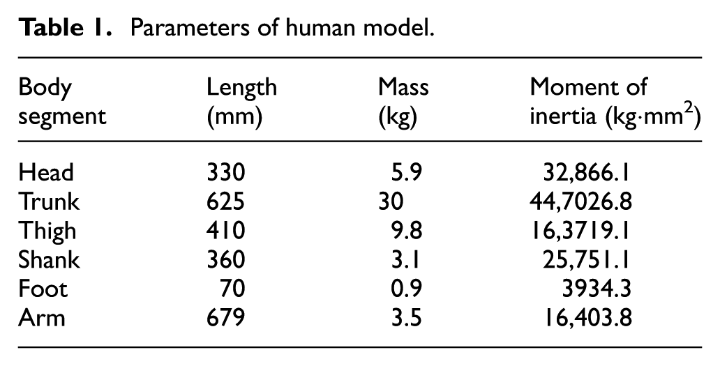
Figure 5 shows the established human model. The parameters of each body segment are given in Table 1. The joint pairs of the upper and lower extremity are added in accordance with the functional relationship during the actual walking. The fixed pair is added between the head and the upper torso so that the two objects do not produce relative motion. The rotational pair constrains objects to rotate around the axis of rotation and a rotational pair is added between the arms and the torso; the hip, knee and ankle joints are added with the rotational pairs. The translational pair constrains two objects to slide only along a sliding axis. The normal walking of human is mainly in the sagittal plane, so the translational pair is added to the upper torso for simulation.

Angle-driven simulation gait diagram.
Parameters of human model.
The angles of lower extremity joint in the gait cycle are measured by VICON three-dimensional gait analysis system. The measured angle data are saved and imported into spline function curve in ADAMS. The motion driver is added to each joint of the lower extremities, and each spline curve is associated with the joint by the CUBSPL function. The simulated walking gait is shown in Figure 5.
In the post-processing module of ADAMS, the joint angles of the simulation are exported and compared with the desired angles, as shown in Figures 6–8.

Comparison of measured and simulated hip joint angles.

Comparison of measured and simulated knee joint angles.

Comparison of measured and simulated ankle joint angles.
The frequency of measured data is different from that of simulated data, so the number of data obtained in the gait cycle is different. First, the two sets of data are normalized and compared in the same gait cycle. And the human locomotion satisfies the smooth characteristics. To calculate the errors between joint angles, the Fourier series is introduced to fit the simulated data curve. Then, the gait cycle variables of the measured data are input into the fitting curve to obtain the fitted joint angle of simulation, and the errors are obtained by subtracting them.
The curve fit toolbox of MATLAB is used to obtain the parameters of simulated trajectory. The Fourier series expression of simulated angles can be expressed as follows
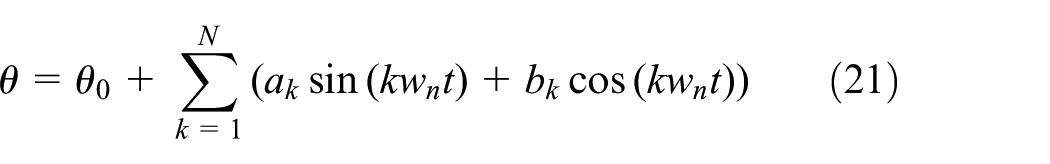
where
Take the hip joint angles as an example. In order to fit the simulation data better, the forth-order harmonics is selected. And the parameters obtained by MATLAB fitting are illustrated in Table 2.
Fourier series fitting parameters of hip angle.
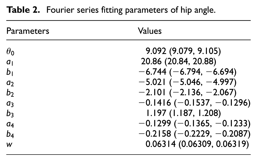
The root mean square error (RMSE) of the fitting result is 0.094, which indicates that the fitting result is representative. The gait cycle variables of the measured data are input to obtain the fitted joint angle of simulation, and the errors of hip joint angles are obtained by subtracting them. The calculation results show that the errors between the simulated joint angle and the desired angle are hip = 2.03%, knee = 1.63%, and ankle = 3.6%, respectively. The errors obtained are within the allowable range, which indicates the correctness of the established human model.
Verification of knee exoskeleton control
Using two “Link” rods to establish a simplified lower limb knee joint exoskeleton, ADAMS software can abstract the functional connection of practical device into a logical relationship. Meanwhile, we add rotating pairs between the rod and the upper torso and two rods, respectively, to simulate the practical rotation. In fact, the power of knee joint is provided by motor, so the knee joint torque is added to simulate the output torque of actual motor.
The control platform of the system is established in MATLAB/Simulink, and the input and output variables of the model are defined in ADAMS. The input variable is the knee joint torque controlled by the MATLAB and the output variable is the knee joint angle of the model in ADAMS. The interface of established model is exported to MATLAB. The input torque calculated by MATLAB and the output angle of ADAMS can exchange through the interface in real time.
Figure 9 shows the control diagram in MATLAB/Simulink. The proposed control algorithm is written into Simulink’s S-Function as a controller, and the ADAMS model interface acts as the controlled object. The actual measured angles serve as the desired input.

MATLAB/Simulink simulation diagram.
For the human–exoskeleton model, the control torque calculated by MATLAB/Simulink system is used to drive the knee joint, and the other joints are driven by the measured joint angles. Figure 10 shows the human walking gait diagram obtained by simulation. The parameters of the controller are shown in Table 3.

Simulation gait diagram of wearing exoskeleton.
Parameters of controller.

MFAC: model-free adaptive control.
The normal walking time of the three gait cycles is selected as the simulation time. We have compared the proposed method with the MFAC method. As shown in Figures 11 and 12, the simulation results show that the proposed method has better performance than the MFAC method. Due to the initialization of the model, the knee angle converges from 42° to the desired angle at the beginning of simulation. According to whether the foot is in contact with the ground, the gait cycle can be divided into two phases: the support phase and the swing phase. MFAC method combined discrete sliding mode, and prior torque has smaller tracking error than MFAC in support phase. After initialization of the model, the maximum error between the desired angle and the output angle of the proposed method is 3°, and the maximum error of the MFAC is 12°.

Comparison of tracking performance between MFAC and MFAC combined discrete sliding mode and prior torque.

Comparison of tracking error between MFAC and MFAC combined discrete sliding mode and prior torque.
The change of angle is that the knee flexion angle increases with a small amplitude at the initial support phase and decreases as the human body moves forward in the mid-support phase. During the swing phase, the knee joint angle is gradually increased, and after reaching the maximum value, the angle is gradually decreased to prepare for foot landing. The acquired knee joint angle in the experiment shows that the knee joint angle ranges from 6.71° to 65.11° during the gait cycle. If the knee joint angle is less than 6.71°, it will cause lower extremity discomfort, and when the angle is negative, it will cause harm to human. The simulation of Figure 11 illustrates that the knee joint angle is within normal range under the proposed control algorithm.
Under the adjustment of the controller, the control torque can be assisted to the human body model, and the torque of the human body acting on the exoskeleton is relatively small. The simulation results show that the proposed method has better performance than the MFAC method. It means that the torque controlled by the proposed method is better than MFAC method in assisting the human model during swing phase, and the torque of the human body acting on the exoskeleton is smaller. The introduction of discrete sliding mode control law and prior torque improves the accuracy and robustness of the system and enables the exoskeleton leg to track the desired trajectory better when it changes rapidly during the swing phase.
Conclusion
Aiming at the control of the knee joint exoskeleton during walking, a MFAC method based on system input and output angle was proposed. The discrete sliding mode law and the prior torque were introduced to improve the control quality. Then, the MATLAB and ADAMS experimental co-simulation platform was designed to test the established human model and control method, respectively. The simulation results show that the method presented in this article has a good performance on the control of the knee exoskeleton during walking.
Footnotes
Appendix 1
The proof that system (6) is transformed into a FFDL model is detailed in the following.
Equation (6) can be expressed as
Equation (23) can be derived from equations (7) and (22)
In order to simply the expression, we denote
By virtue of Assumption 1 and Cauchy differential mean value theorem, equation (22) can be rewritten as
where
Since condition
Equation (23) can be deduced to
Equation (9) is proved.
Handling Editor: Emre Sariyildiz
Declaration of conflicting interests
The author(s) declared no potential conflicts of interest with respect to the research, authorship, and/or publication of this article.
Funding
The author(s) disclosed receipt of the following financial support for the research, authorship, and/or publication of this article: This article was supported by the National Natural Science Foundation of China (61773151 and 61703134) and the Natural Science Foundation of Hebei Province (F2018202279).