Three non-Newtonian fluids flow considering thin film over an unsteady stretching surface with variable fluid properties

Abstract

This research examines the features of liquid film of non-Newtonian fluids under the influence of thermophoresis. For this study, we proposed a mathematical model for Jeffrey, Maxwell, and Oldroyd-B fluids and concluded the unsteady stretched surface in the existence of a magnetic field and also the thermal conductivity was measured which is directly related to the temperature whereas the viscosity inversely related to the temperature. Inserting the thermophoretic effect which improved the thermal conductivity of Jeffrey fluid over the Oldroyd-B and Maxwell fluids. The model is helpful for the liquid flow of Jeffrey, Maxwell, and Oldroyd-B fluid including the Brownian motion parameter effect. The results have been obtained through optimal approach compared with numerical (ND-Solve) method. Study mainly focused to understand the physical appearance of the embedded parameters based on the characteristic length of the liquid flow. The behavior of skin friction, local Nusselt number, and Sherwood number has been described numerically for the dynamic constraints of the problem. The obtained results are drafted graphically and discussed.

Introduction

The flow analysis of thin film flow has got significant devotion due to its gigantic usages and application in the area of industries, engineering, and technology in a recent few years. Thin film flow problems were seen in many fields, fluctuating from specific situations in the flow in human lungs to lubrication problems in engineering, which is probably one of the largest subfield of thin film flow problems. The exploration of thin film flow of practical applications is a challenging interplay between fluid mechanics, structural mechanics, and theology. Wire and fiber coating is one of its important applications. Extrusion of polymer and metal, processing of food stuff, continuous casting, plastic sheets drawing, and fluidization of reactor, exchanges, and chemical processing equipment are some of its well-known applications. In view of these applications, it becomes an important issue for researchers to develop the study of liquid film on a stretching surface. The flow of liquid film was first studied for viscous flow and furthermore, it is extended to non-Newtonian fluid. Crane ¹ was the first one who deliberated the motion of viscid fluid in a linear stretching surface.Dandapat and Gupta ² studied the flow of viscoelastic fluids on a stretching surface with heat transfer. Wang ³ was the first one to investigate finite liquid film on time-dependent stretched surface. Usha and Sridharan ⁴ worked on the same problem and extended it to liquid film fluid with heat transmission analysis of horizontal sheet. Liu and Andersson ⁵ used the numerical techniques in their work to obtain a solution and discussed the physical parameters of the problem. Aziz et al. ⁶ observed the consequence of inner heat production on a thin liquid film flow on a time depending stretching sheet. Recently, Tawade et al. ⁷ inspected thin liquid flow over an instable extending sheet with thermal radioactivity, in the existence of magnetic field, using the Runge-Kutta–Fehlberg and Newton–Raphson method for solution of non-linear equations. A brief discussion is given on physical parameters in his work.

Megahed ⁸ examined thin film flow of Casson fluid and heat transmission in the existence of inconstant heat flux and viscid dissipation with slip velocity. Abolbashari et al. ⁹ inspected the same fluid with entropy generation. Qasim et al. ¹⁰ studied the fluid film on an unsteady stretching sheet taking Buongiorno’s model. Maxwell fluid is an important subclass of non-Newtonian fluids. Several researchers investigated Maxwell fluid with the effect of heat and magnetohydrodynamics (MHD). Hayat et al. ¹¹ deliberated boundary coating flow of Maxwell nanofluid in three dimensions. Stanford Shateyi ¹² investigated Maxwell fluid with the new numerical approach in the existence of MHD. Swati Mukhopadhyay ¹³ examined the same fluid and also considered the consequence of heat source and sink in unsteady shrinking sheet. Nadeem et al. ¹⁴ investigated numerically MHD Maxwell fluid in preceding extending sheet in the occurrence of MHD. Nadeem et al. ¹⁵ also study the boundary layer flow and heat transfer of a Maxwell fluid over an exponential stretching surface with thermal stratifications. The consequence of homogeneous and heterogeneous response is incorporated. Cattaneo–Christov heat flux model is used instead of the Fourier law of heat conduction, which is recently proposed by Christov.

In engineering and technological fields, most of mathematical problems are complex in their nature and the exact solution is almost very difficult or even not possible to obtain. So for the solution of such problems, numerical and analytical methods are used to find the approximate solution. One of important and popular techniques for the answering of such type problems is the homotopy analysis method. It is a substitute method and its main advantage is applying it to the non-linear differential equations without discretization and linearization. Liao^16–23 was the first one to investigate this technique for the solution of that type problems and generally proved that this method is rapidly converging to the approximated solutions. Also, this method provides series solutions in the form of functions of a single variable. Solution with this method is important because it involves all the physical parameters of the problem and we can easily discuss its behavior. Due to its fast convergence, many researchers like Rashidi and Pour, ²⁴ Abbasbandy, ²⁵ Abbasbandy,^25–27 Hayat et al., ^28,29 and Nadeem and colleagues^30,31 used this procedure to answer for the highly non-linear combined equations. Mehmood et al. ³² investigate the problem of oblique stagnation point flow using Jeffery nanofluid as a rheological fluid model. The thermophoresis and Brownian motion consequences are taken. Resulting highly non-linear system of differential equations is solved numerically through mid-point integration and by optimal homotopy asymptotic method (OHAM). Raju et al. ³³ investigated the combined study of Jeffrey, Maxwell, and Oldroyd-B fluids on the surface of Cone using steady case. The thermophoretic and Brownian effect has been studied in their work. Sandeep and Sulochana, ³⁴ and Sandeep and Malvandi ³⁵ studied the flow of the Jeffrey, Maxwell, and Oldroyd-B fluid flow over steady and unsteady stretching surfaces. Mukhopadhyay and Bhattacharyya ³⁶ examined the flow of Maxwell fluid over an unsteady stretching surface. The effect of various parameters has been studied in their work.

In all of the discussed work, researchers consider heat and mass transmission features of Newtonian or non-Newtonian fluid at a time-dependent or time-independent stretching surface taking one or more physical characteristics. The momentum equation has been used as Sandeep and Malvandi, ³⁵ while the energy and concentration equations are used as in Qasim et al. ¹⁰ The main focus has been given to the variable fluid properties under the effect of temperature. To the best of the author’s knowledge, no studies have been described, nevertheless, on studying the flow of heat and mass transmission features of thermophoretic liquid film flow of non-Newtonian nanofluids with temperature reliant viscosity and thermal conductivity. The main aim of this work is to investigate the liquid film flow of Jeffrey, Maxwell, and Oldroyd-B fluids over an unsteady stretched surface in the existence of magnetic field and non-uniform heat transmission. Keeping in view these assumptions, taken into the model problems and the similarity transformation method, the concerned PDEs are converted to non-linear ODEs, and the obtained, transformed equations are analytically solved using HAM; the Numerical method is also used for the comparison of these solutions.

Problem formulation

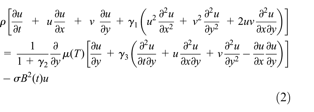
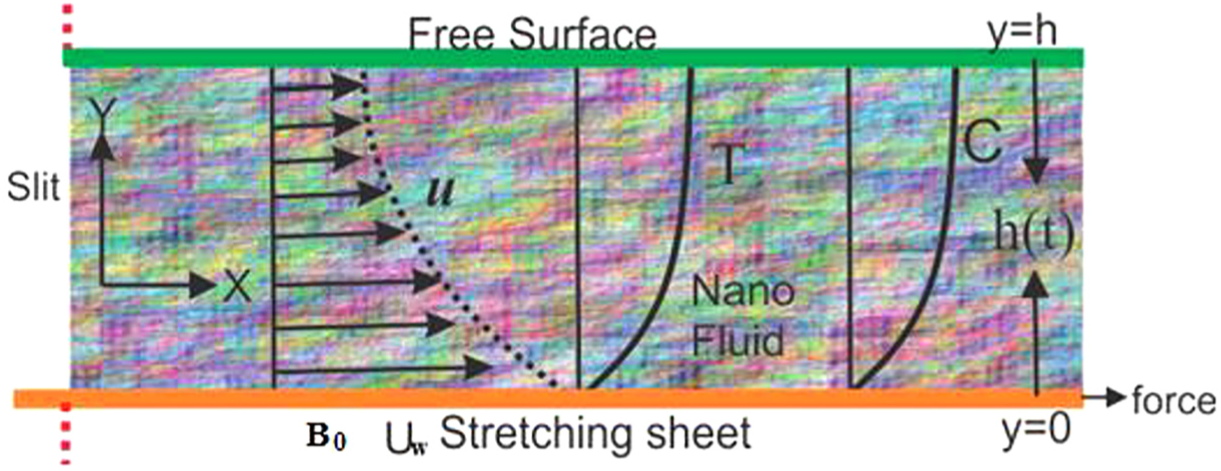
Consider a time-dependent liquid film flow of magnetohydrodynamic Jeffrey, Maxwell, and Oldroyd-B fluids for stretching sheet. The viscosity and thermal conductivity of the fluids varies with temperature. The Cartesian accommodates system $\mathrm{oxyz}$ is adjusted in a well-known manner that $\mathrm{ox}$ is parallel to the plate and $\mathrm{oy}$ is perpendicular to the sheet. The surface of the flow is stretched by applying two equivalent and reverse forces along the $x\mathrm{-}\mathrm{axis}$ to keep the origin stationary. The $x\mathrm{-}\mathrm{axis}$ is taking along the stretching surface with stretch velocity $U_w(x,t)=\mathrm{bx}/1-\mathrm{at}$ , in which a, b are constant and y-axis is perpendicular to it, in which $b>0$ , is the stretching velocity constraint and if $b<0$ then it will become shrinking velocity constraint. $T_w(x,t)=T_0-T_r(b{x}^2/2\upsilon )(1-\mathrm{at}{)}^{-1.5}$ is the wall temperature of the fluid, and $C_w(x,t)=C_0-$ $C_r(b{x}^2/2\upsilon )(1-\mathrm{at}{)}^{-1.5}$ indicates the nanoparticle capacity portion, $\upsilon$ represents the kinematic viscidness of the fluid, and $T_0,T_r$ slit and reference temperatures, respectively, while $C_0,C_r$ are the slit and reference volume fraction of particle, respectively. A magnetic field $B(t)=B_0(1-\mathrm{at}{)}^{-0.5}$ is given normally to the stretching sheet, as shown in Figure 1. The momentum equation is used as in the work of Sandeep and Malvandi ³⁵ with the addition of variable viscosity, while the energy and concentration equation with the addition of variable thermal conductivity are used as in the work of Qasim et al. ¹⁰ For the Brownian motion. The continuity equation, the elementary boundary governing equation, heat transferring and concentration equations can be stated as

$$\frac{\partial u}{\partial x}+\frac{\partial v}{\partial y}=0$$

(1)

$$\begin{array}{c}\rho [\frac{\partial u}{\partial t}+u\frac{\partial u}{\partial x}+v\frac{\partial u}{\partial y}+{\gamma }_1(u^2\frac{{\partial }^{2}u}{\partial x^2}+v^2\frac{{\partial }^{2}u}{\partial y^2}+2\mathrm{uv}\frac{{\partial }^{2}u}{\partial x\partial y})]\hfill \\ =\frac{1}{1+{\gamma }_2}\frac{\partial }{\partial y}\mu (T)[\frac{\partial u}{\partial y}+{\gamma }_3(\frac{{\partial }^{2}u}{\partial t\partial y}+u\frac{{\partial }^{2}u}{\partial x\partial y}+v\frac{{\partial }^{2}u}{\partial y^2}-\frac{\partial u}{\partial x}\frac{\partial u}{\partial y})]\hfill \\ -\sigma B^2(t)u\hfill \end{array}$$

(2)

$$\begin{array}{c}\frac{\partial T}{\partial t}+u\frac{\partial T}{\partial x}+v\frac{\partial T}{\partial y}=\frac{1}{\left(\rho c_p\right)}\frac{\partial }{\partial y}[K(T)\frac{\partial T}{\partial y}]\hfill \\ +\tau [D_B\left(\frac{\partial C}{\partial y}\frac{\partial T}{\partial y}\right)+\frac{D_T}{T_1}{\left(\frac{\partial T}{\partial y}\right)}^2]\hfill \end{array}$$

(3)

$$[\frac{\partial C}{\partial t}+u\frac{\partial C}{\partial x}+v\frac{\partial C}{\partial y}]=D_B\frac{{\partial }^{2}C}{\partial y^2}+\left(\frac{D_T}{T_1}\right)\frac{{\partial }^{2}T}{\partial y^2}$$

(4)

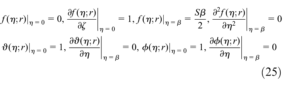
The applicable boundaries constrains for the flow pattern are taken

$$u=U_w,v=0,T=T_w,C=C_w\mathrm{at}y=0$$

(5)

$$\frac{\partial u}{\partial x}=0,\frac{\partial T}{\partial x}=0,\frac{\partial C}{\partial x}=0,v=\frac{\mathrm{dh}}{\mathrm{dt}}\mathrm{at}y=h$$

(6)

in which $u$ and $v$ indicate the velocities constituents alongside x- and y-axes correspondingly; $\mu (T)={\mu }_0{e}^{-m(T-T_0)}$ represents the variable viscosity of the fluid such that $\mathrm{\Lambda }=m(T_w-T_0)$ ; $\sigma$ is the electric conductive parameter of fluid; ${\gamma }_1,{\gamma }_2,{\gamma }_3$ represent the relaxation time, ratio of the relaxation to retardation time, and retardation time, respectively. cmagneticzes the applied magnetic field, T is the local temperature, $\rho$ is the fluid density, $c_p$ represents the heat capacitanin, which fluid, where is the variable thermal conductivity is defined as $K(T)=K_0{e}^{c(T-T_0)}$ in which $\epsilon =c(T-T_0)$ is used for flexible thermal conductivity constraint, $\tau$ heat capacities, $D_B$ directs the Brownian diffusion constant, while the thermophoretic diffusion constant is represented by $D_T$ , $T_{\infty }$ represents the temperature of the fluid with large distant from the surface, C is the local particle volume fraction, $T_m$ represents the mean temperature.

Figure 1.

The physical configuration of the modeled problems.

Equation (2) deals with different film flow models based on the following conditions^33–35:

1. Jeffrey fluid: ${\gamma }_1=0,{\gamma }_2\ne 0,{\gamma }_3\ne 0$ ;

2. Maxwell fluid: ${\gamma }_1\ne 0,{\gamma }_2=0,{\gamma }_3=0$ ;

3. Oldroyd-B fluid: ${\gamma }_1\ne 0,{\gamma }_2=0,{\gamma }_3\ne 0$ .

Using similarity transformations

$$\begin{array}{c}\psi =x\sqrt{\upsilon b/(1-\mathrm{at})}f\left(\eta \right),u=\partial \psi /\partial y=\mathrm{bx}/(1-\mathrm{at})f\prime \left(\eta \right),\hfill \\ v=-\partial \psi /\partial x=-\sqrt{\upsilon b/(1-\mathrm{at})}f\left(\eta \right)\hfill \\ \eta =\sqrt{b/\upsilon (1-\mathrm{at})}y,h=\sqrt{\upsilon (1-\mathrm{at})/b},\hfill \\ \vartheta (\eta )=(T-T_0)/(T_w-T_0),\varphi (\eta )=(C-C_0)/(C_w-C_0)\hfill \end{array}$$

(7)

where prime specifies the derivative with respect to $\eta$ and $\psi$ indicates the stream function; $h(t)$ specifies the liquid film thickness and $\upsilon =\mu /\rho$ is the kinematics viscosity. The dimensionless film thickness $\beta =\sqrt{b/\upsilon (1-\mathrm{at})}h(t)$ which gives $\mathrm{dh}/\mathrm{dt}=-a\beta /2\sqrt{\upsilon /b(1-\mathrm{at})}$ is given Wang ³ and Qasim et al. ¹⁰

Using the similarity transformation equation (7) into equations (1)–(6) satisfies the continuity equation, while the remaining equations are transformed into system of non-linear differential system of equations as

$$\begin{array}{c}\frac{1}{(1+{\delta }_2)}[f″\prime +{\delta }_3\{{(f″)}^2-f{f}^{\mathrm{iv}}+S(2f″\prime +\frac{\eta }{2}{f}^{\mathrm{iv}})-{\epsilon }_3\mathrm{Mf}\prime \}]\hfill \\ +(1+\mathrm{\Lambda }\vartheta )[\mathrm{ff}″-{(f\prime )}^2-S(2f\prime +\frac{\eta }{2}f″)-{\delta }_1({\left(f\right)}^{2}f″\prime -2\mathrm{ff}\prime f″)]=0\hfill \end{array}$$

(8)

$$\begin{array}{c}(1+\epsilon \vartheta )\vartheta ″\hfill \\ +\mathrm{Pr}(f\vartheta \prime -2f\prime \vartheta -\frac{S}{2}(3\vartheta +\eta \vartheta \prime )+N_t{(\vartheta \prime )}^2+N_b\vartheta \prime \varphi \prime )\hfill \\ =0\hfill \end{array}$$

(9)

$$\varphi ″+S_c[f\varphi \prime -2f\prime \varphi -\frac{S}{2}(3\varphi +\eta \varphi \prime )]+\frac{N_t}{N_b}\vartheta ″=0$$

(10)

The boundary constrains of the problem are

$$\begin{array}{c}f(0)=0,f\prime (0)=1,\vartheta (0)=1,\varphi (0)=1,\hfill \\ f(\beta )=\frac{S\beta }{2},f″(\beta )=0,\vartheta \prime (\beta )=0,\varphi \prime (\beta )=0\hfill \end{array}$$

(11)

The physical constraints after generalization

Where ${\delta }_1,{\delta }_2,{\delta }_3$ represent the Deborah quantities of relaxation time, ratio of relaxation, retardation, and retardation time, respectively; $\mathrm{S}=a/b$ represents the dimensional less measure of instability; ${\epsilon }_3$ is the fluid constants; $M=\sigma B_0^2/b\rho$ represents the magnetic field parameter; $\mathrm{\Lambda }=m(T_w-T_0)$ represents the variable viscosity parameter; $\mathrm{Pr}=\upsilon (\rho c_p)/k$ is the Prandtl number; $N_t=\tau D_w(T_w-T_0)/\upsilon T_0$ represents thermophoresis constraint; $N_b=\tau D_B(C_w-C_0)/\upsilon$ indicates Brownian motion limitation; $S_c=\upsilon /D_B$ is used for Schmidt number and all of these are defined respectively.

The coefficient of skin friction is given by

$$C_f=\frac{{\left({\tau }_{\mathrm{xy}}\right)}_{y=0}}{\rho U_w^2}$$

(12)

$$\begin{array}{c}\multicolumn{1}{c}{\left({\tau }_{\mathrm{xy}}\right)={\gamma }_1(u^2\frac{{\partial }^{2}u}{\partial x^2}+v^2\frac{{\partial }^{2}u}{\partial y^2}+2\mathrm{uv}\frac{{\partial }^{2}u}{\partial x\partial y})}\\ -\frac{1}{1+{\gamma }_2}\frac{\partial }{\partial y}\mu (T)\hfill \\ [\frac{\partial u}{\partial y}+{\gamma }_3(\frac{{\partial }^{2}u}{\partial t\partial y}+u\frac{{\partial }^{2}u}{\partial x\partial y}+v\frac{{\partial }^{2}u}{\partial y^2}-\frac{\partial u}{\partial x}\frac{\partial u}{\partial y})]\hfill \end{array}$$

(13)

Substituting the non-dimensional variables from equation (8) into equations (1)–(7), it reduced to the form of

$$R{e^{-\frac{1}{2}}}_x{C}_f=\frac{1+{\gamma }_1}{1+{\gamma }_2}f″(0)$$

(14)

where $R{e}_x=U_{w}x/\nu$ and it is called the local Reynolds number. The Nusselt number $\mathrm{Nu}$ is defined as $\mathrm{Nu}=d{Q}_w/\hat{k}(T-T_d)$ in which $Q_w$ represents the heat flux where $Q_w=-\hat{k}(\partial T/\partial y{)}_{\eta =0}$ . The Sherwood number is defined as $\mathrm{Sh}=D{J}_w/\hat{k}(T-T_d)$ , in which $J_w$ is the mass flux where $J_w=-D(\partial C/\partial y{)}_{\eta =0}$ . The dimensionless form of $\mathrm{Nu}$ and $\mathrm{Sh}$ is obtained as

$$\mathrm{Nu}=-(1+\epsilon \theta (0))\theta \prime (0),\mathrm{Sh}=-\varphi \prime (0)$$

(15)

Solution by HAM

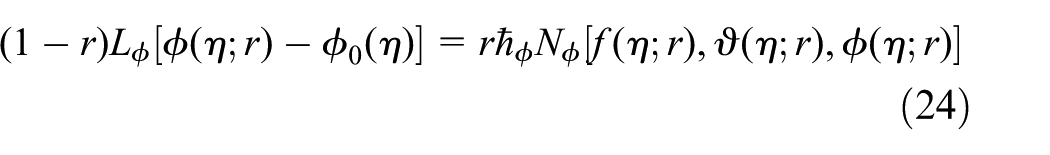
Equations (8)–(10) corresponding the boundary constrain (11) is approximately solved with homotopy analysis method (HAM) the subsequent technique is applied. The solutions enclosed the auxiliary parameters $\hslash$ which control and converge the solutions.

The initial solution is given as follows

$$\begin{array}{c}\multicolumn{1}{c}{f_0(\eta )=\frac{1}{4{\beta }^2}(4{\beta }^2\eta +3\beta (S-2){\eta }^2+(2-S){\eta }^3),}\\ {\vartheta }_0(\eta )={\eta }^2-2\beta \eta ,{\varphi }_0(\eta )={\eta }^2-2\beta \eta \hfill \end{array}$$

(16)

The linear operators are represented by

$$L_f(f)=f^{\mathrm{iv}},L_{\vartheta }(\vartheta )=\vartheta ″,L_{\varphi }(\varphi )=\varphi ″$$

(17)

which has the subsequent applicability

$$\begin{array}{c}{L}_f(e_1+e_2\eta +e_3{\eta }^2+e_4{\eta }^3)=0,L_{\vartheta }(e_5+e_6\eta )=0\hfill \\ \mathrm{and}{L}_{\varphi }(e_7+e_8\eta )=0\hfill \end{array}$$

(18)

where $e_i(i=1->8)$ the coefficients involve in the solution.

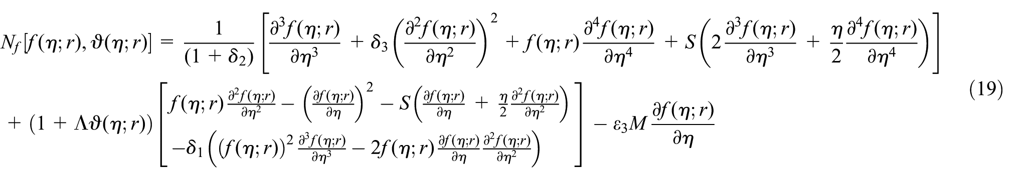
The corresponding non-linear operators $N_f,N_{\vartheta },N_{\varphi }$ are carefully chosen of the form

$$\begin{array}{c}{N}_f[f(\eta ;r),\vartheta (\eta ;r)]=\frac{1}{(1+{\delta }_2)}[\frac{{\partial }^{3}f(\eta ;r)}{\partial {\eta }^3}+{\delta }_3{\left(\frac{{\partial }^{2}f(\eta ;r)}{\partial {\eta }^2}\right)}^2+f(\eta ;r)\frac{{\partial }^{4}f(\eta ;r)}{\partial {\eta }^4}+S(2\frac{{\partial }^{3}f(\eta ;r)}{\partial {\eta }^3}+\frac{\eta }{2}\frac{{\partial }^{4}f(\eta ;r)}{\partial {\eta }^4})]\hfill \\ +(1+\mathrm{\Lambda }\vartheta (\eta ;r))\left[\begin{array}{c}f(\eta ;r)\frac{{\partial }^{2}f(\eta ;r)}{\partial {\eta }^2}-{\left(\frac{\partial f(\eta ;r)}{\partial \eta }\right)}^2-S(\frac{\partial f(\eta ;r)}{\partial \eta }+\frac{\eta }{2}\frac{{\partial }^{2}f(\eta ;r)}{\partial {\eta }^2})\hfill \\ \multicolumn{1}{c}{-{\delta }_1({(f(\eta ;r))}^2\frac{{\partial }^{3}f(\eta ;r)}{\partial {\eta }^3}-2f(\eta ;r)\frac{\partial f(\eta ;r)}{\partial \eta }\frac{{\partial }^{2}f(\eta ;r)}{\partial {\eta }^2})}\end{array}\right]-{\epsilon }_{3}M\frac{\partial f(\eta ;r)}{\partial \eta }\hfill \end{array}$$

(19)

$$\begin{array}{c}{N}_{\vartheta }[f(\eta ;r),\vartheta (\eta ;r),\varphi (\eta ;r)]=(1+\epsilon \vartheta (\eta ;r))\frac{{\partial }^2\vartheta (\eta ;r)}{\partial {\eta }^2}\hfill \\ +\mathrm{Pr}\left(\begin{array}{c}f(\eta ;r)\frac{\partial \vartheta (\eta ;r)}{\partial \eta }-2\frac{\partial f(\eta ;r)}{\partial \eta }\vartheta (\eta ;r)-\frac{S}{2}(3\vartheta (\eta ;r)+\eta \frac{\partial \vartheta (\eta ;r)}{\partial \eta })\hfill \\ \multicolumn{1}{c}{+N_t{\left(\frac{\partial \vartheta (\eta ;r)}{\partial \eta }\right)}^2+N_b\frac{\partial \vartheta (\eta ;r)}{\partial \eta }\frac{\partial \varphi (\eta ;r)}{\partial \eta }}\end{array}\right)\hfill \end{array}$$

(20)

$$\begin{array}{c}{N}_{\varphi }[f(\eta ;r),\vartheta (\eta ;r),\varphi (\eta ;r)]=\frac{{\partial }^2\varphi (\eta ;r)}{\partial {\eta }^2}\hfill \\ +S_c[f(\eta ;r)\frac{\partial \varphi (\eta ;r)}{\partial \eta }-2\frac{\partial f(\eta ;r)}{\partial \eta }\varphi (\eta ;r)]\hfill \\ -\frac{S}{2}(3\varphi (\eta ;r)+\eta \frac{\partial \varphi (\eta ;r)}{\partial \eta })+\frac{N_t}{N_b}\frac{{\partial }^2\vartheta (\eta ;r)}{\partial {\eta }^2}\hfill \end{array}$$

(21)

The elementary solution procedure by HAM is defined in the previous works,^20–26 the 0th order system form equations (8)–(10) as

$$(1-r)L_f[f(\eta ;r)-f_0(\eta )]=r{\hslash }_f{N}_f[f(\eta ;r),\vartheta (\eta ;r)]$$

(22)

$$(1-r)L_{\vartheta }[\vartheta (\eta ;r)-{\vartheta }_0(\eta )]=r{\hslash }_{\vartheta }{N}_{\vartheta }[f(\eta ;r),\vartheta (\eta ;r),\varphi (\eta ;r)]$$

(23)

$$(1-r)L_{\varphi }[\varphi (\eta ;r)-{\varphi }_0(\eta )]=r{\hslash }_{\varphi }{N}_{\varphi }[f(\eta ;r),\vartheta (\eta ;r),\varphi (\eta ;r)]$$

(24)

The correspondent boundary constrains are

$$\begin{array}{c}{f(\eta ;r)|}_{\eta =0}=0,{\frac{\partial f(\eta ;r)}{\partial \zeta }|}_{\eta =0}=1,{f(\eta ;r)|}_{\eta =\beta }=\frac{S\beta }{2},{\frac{{\partial }^{2}f(\eta ;r)}{\partial {\eta }^2}|}_{\eta =\beta }=0\hfill \\ {\vartheta (\eta ;r)|}_{\eta =0}=1,{\frac{\partial \vartheta (\eta ;r)}{\partial \eta }|}_{\eta =\beta }=0,{\varphi (\eta ;r)|}_{\eta =0}=1,{\frac{\partial \varphi (\eta ;r)}{\partial \eta }|}_{\eta =\beta }=0\hfill \end{array}$$

(25)

where $r\in [0,1]$ is the imbedding constraint; ${\hslash }_f,{\hslash }_{\vartheta },\mathrm{and}{\hslash }_{\varphi }$ are used to regulate for solution convergence. When $r=0\mathrm{and}\mathrm{r}=1$ , we have

$$f(\eta ;1)=f(\eta ),\vartheta (\eta ;1)=\vartheta (\eta )\mathrm{and}\varphi (\eta ;1)=\varphi (\eta )$$

(26)

Expand the velocity, temperature, and concentration field, $f(\eta ;r),\vartheta (\eta ;r),\varphi (\eta ;r)$ in Taylor’s series approximately $r=0$

$$\begin{array}{c}\multicolumn{1}{c}{f(\eta ;r)=f_0(\eta )+\sum _{n=1}^{\infty }{f}_n(\eta )r^n,\vartheta (\eta ;r)={\vartheta }_0(\eta )}\\ +\sum _{n=1}^{\infty }{\vartheta }_n(\eta )r^n,\varphi (\eta ;r)={\varphi }_0(\eta )\hfill \\ +\sum _{n=1}^{\infty }{\varphi }_n(\eta )r^n\hfill \end{array}$$

(27)

where

$$\begin{array}{c}{f}_n(\eta )=1/n!\left({\partial f(\eta ;r)/\partial \eta |}_{r=0}\right),\hfill \\ {\theta }_n(\eta )=1/n!\left({\partial \vartheta (\eta ;r)/\partial \eta |}_{r=0}\right)\mathrm{and}\hfill \\ {\varphi }_n(\eta )=1/n!\left({\partial \varphi (\eta ;r)/\partial \eta |}_{r=0}\right)\hfill \end{array}$$

(28)

The secondary restrictions ${\hslash }_f,{\hslash }_{\vartheta },\mathrm{and}{\hslash }_{\varphi }$ are chosen in a manner that series (27) converges at $r=1$ , switching $r=1$ in equation (27), we obtain

$$\begin{array}{c}\multicolumn{1}{c}{f(\eta )=f_0(\eta )+\sum _{n=1}^{\infty }{f}_n(\eta ),\vartheta (\eta )={\vartheta }_0(\eta )}\\ +\sum _{n=1}^{\infty }{\vartheta }_n(\eta ),\varphi (\eta )={\varphi }_0(\eta )+\sum _{n=1}^{\infty }{\varphi }_n(\eta )\hfill \end{array}$$

(29)

The nth order system of equations is

$$\begin{array}{c}{L}_f[f_n(\eta )-{\chi }_n{f}_{n-1}(\eta )]={\hslash }_f{R}_n^f(\eta ),\hfill \\ L_{\vartheta }[{\vartheta }_n(\eta )-{\chi }_n{\vartheta }_{n-1}(\eta )]={\hslash }_{\vartheta }{R}_n^{\vartheta }(\eta ),\hfill \\ L_{\varphi }[{\varphi }_n(\eta )-{\chi }_n{\varphi }_{n-1}(\eta )]={\hslash }_{\varphi }{R}_n^{\varphi }(\eta )\hfill \end{array}$$

(30)

The consistent boundary conditions are

$$\begin{array}{c}\multicolumn{1}{c}{f_n(0)=f{\prime }_n(0)={\vartheta }_n(0)={\varphi }_n(0)=0,}\\ \multicolumn{1}{c}{f_n(\beta )={f″}_n(\beta )=\vartheta {\prime }_n(\beta )=\varphi {\prime }_n(\beta )=0}\end{array}$$

(31)

Here

$$\begin{array}{c}{R}_n^f(\eta )=\frac{1}{(1+{\delta }_2)}[{f″\prime }_{n-1}+{\delta }_3(\sum _{k=0}^{n-1}{f″}_{n-1-k}{f″}_k-\sum _{k=0}^{n-1}{f}_{n-1-k}{f″″}_k-)+S(2{f″\prime }_{n-1}+\frac{\eta }{2}{f″″}_{n-1})]\hfill \\ +\left[\begin{array}{c}\sum _{k=0}^{n-1}{f}_{n-1-k}{f″}_k-\sum _{k=0}^{n-1}{f\prime }_{n-1-k}{f\prime }_k-S(2{f\prime }_{n-1}+\frac{\eta }{2}{f″}_{n-1})\hfill \\ \multicolumn{1}{c}{-{\delta }_1(\sum _{k=0}^{n-1}{f}_{n-1-k}\sum _{l=0}^k{f}_{k-l}{f″\prime }_l-2\sum _{k=0}^{n-1}{f}_{n-1-k}\sum _{l=0}^k{f\prime }_{k-l}{f″}_l)}\end{array}\right]\hfill \\ \mathrm{\Lambda }\left[\begin{array}{c}\sum _{k=0}^{n-1}{f}_{n-1-k}\sum _{l=0}^k{f″}_{k-l}{\vartheta }_l-\sum _{k=0}^{n-1}{f\prime }_{n-1-k}\sum _{l=0}^k{f\prime }_{k-l}{\vartheta }_l\hfill \\ \multicolumn{1}{c}{-S(\sum _{k=0}^{n-1}{f\prime }_{n-1-k}{\vartheta }_k+\frac{\eta }{2}\sum _{k=0}^{n-1}{f″}_{n-1-k}{\vartheta }_k)}\\ \multicolumn{1}{c}{-{\delta }_1(\sum _{k=0}^{n-1}{f}_{n-1-k}\sum _{l=0}^k{f}_{k-l}\sum _{p=0}^1{f″\prime }_{1-p}{\vartheta }_p-2\sum _{k=0}^{n-1}{f}_{n-1-k}\sum _{l=0}^k{f\prime }_{k-l}\sum _{p=0}^1{f″}_{1-p}{\vartheta }_p)}\end{array}\right]-{\epsilon }_{3}M{f\prime }_{n-1}\hfill \end{array}$$

(32)

$$R_n^{\vartheta }(\eta )={\vartheta ″}_{n-1}+\sum _{k=0}^{n-1}{\vartheta }_{n-1-k}{\vartheta ″}_k+\mathrm{Pr}\left(\begin{array}{c}\sum _{k=0}^{n-1}{f}_{n-1-k}{\vartheta \prime }_k-2\sum _{k=0}^{n-1}{f\prime }_{n-1-k}{\vartheta }_k\hfill \\ \multicolumn{1}{c}{-\frac{S}{2}(3{\vartheta }_{n-1}+\eta {\vartheta \prime }_{n-1})+N_t\sum _{k=0}^{n-1}{\vartheta \prime }_{n-1-k}{\vartheta \prime }_k+N_b\sum _{k=0}^{n-1}{\vartheta \prime }_{n-1-k}{\varphi \prime }_k}\end{array}\right)$$

(33)

$$R_n^{\varphi }(\eta )={\varphi ″}_{n-1}+S_c[\sum _{k=0}^{n-1}{f}_{n-1-k}{\varphi \prime }_k-2\sum _{k=0}^{n-1}{f\prime }_{n-1-k}{\varphi }_k-\frac{S}{2}(3{\varphi }_{n-1}+\eta {\varphi \prime }_{n-1})]+\frac{N_t}{N_b}{\vartheta ″}_{n-1}$$

(34)

where ${\chi }_n=\{0,\mathrm{if}\mathrm{r}\le 1\mathrm{and}1,\mathrm{if}\mathrm{r}>1$ .

HAM solution convergence

The convergence of equation (29) was exclusively influenced by the auxiliary constraints ${\hslash }_f,{\hslash }_{\vartheta },\mathrm{and}{\hslash }_{\varphi }$ . It is a selection in a manner that it controls and converges the series solution. The possibility segments of $\hslash$ are plot $\hslash$ curves of $f″(0),\vartheta \prime (0),\mathrm{and}\varphi \prime (0)$ for 24th order approximated HAM solution. The effective region of $\hslash$ is $-3.2<{\hslash }_f<-0.5,-1.7<{\hslash }_{\theta }<-0.4\mathrm{and}-1.6<{\hslash }_{\varphi }<-0.3$ . The convergence of the HAM method through $\hslash$ curves for velocity, temperature, and concentration fields has been shown in Figures 2–4, respectively.

Figure 2.

The graph of $\hslash$ curves for $f″(0)$ when ${\delta }_1=0,{\delta }_2=0.5,{\delta }_3=0.5,S=0.9,{ϵ}_3=0.8,M=0.7,\mathrm{\Lambda }=0.5,\mathrm{Pr}=0.6,\epsilon =1,N_t=0.7,N_b=0.6,S_c=0.6,\beta =1$ .

Figure 3.

The graph of $\hslash$ curves for $\vartheta \prime (0)$ when ${\delta }_1=0,{\delta }_2=0.5,{\delta }_3=0.5,S=0.9,{ϵ}_3=0.8,M=0.7,\mathrm{\Lambda }=0.5,\mathrm{Pr}=0.6,\epsilon =1,N_t=0.7,N_b=0.6,S_c=0.6,\beta =1$ .

Figure 4.

The graph of $\hslash$ curves for $\varphi \prime (0)$ when ${\delta }_1=0,{\delta }_2=0.5,{\delta }_3=0.5,S=0.9,{ϵ}_3=0.8,M=0.7,\mathrm{\Lambda }=0.5,\mathrm{Pr}=0.6,\epsilon =1,N_t=0.7,N_b=0.6,S_c=0.6,\beta =1$ .

Results and discussion

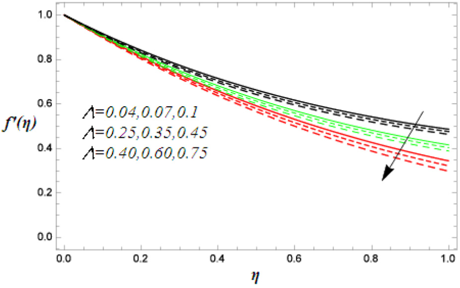
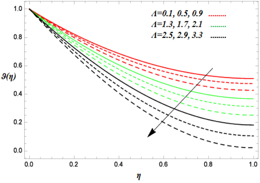
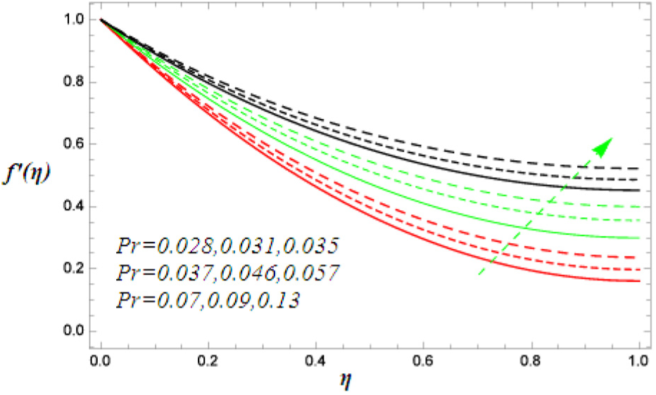
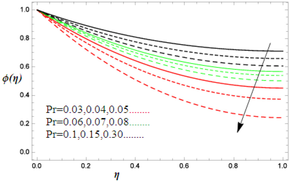
The consequences of several physical parameters, namely, variable viscosity constraint, Prandtl quantity, Schmidt number, liquid film thickness, magnetic field parameter, unsteady parameter, Brownian motion constraint, thermophoresis parameter on velocity, temperature and concentration fields, have been displayed through graphs. The HAM solution has been compared with numerical method (ND-Solve Method) and the agreement of these two techniques has been displayed through graphs and tables. The Jeffery, Maxwell, and Oldroyd-B fluids are presented by red, green, and black colors in Figures 5–23.

Figure 5.

Fluctuations in velocity field $f\prime (\eta )$ for various values of $\mathrm{\Lambda }$ when $h=-0.2,{\delta }_1=0,{\delta }_2=0.5,{\delta }_3=0.5,S=0.9,{ϵ}_3=0.8,M=0.7,\mathrm{Pr}=0.6,\epsilon =1,N_t=0.7,N_b=0.6,S_c=0.6,\beta =1$ .

Figure 6.

Fluctuations in temperature gradient $\vartheta (\eta )$ for various values of $\mathrm{\Lambda }$ when $h=-0.2,{\delta }_1=0,{\delta }_2=0.5,{\delta }_3=0.5,S=0.9,{ϵ}_3=0.8,M=0.7,\mathrm{Pr}=0.6,\epsilon =1,N_t=0.7,N_b=0.6,S_c=0.6,\beta =1$ .

Figure 7.

Fluctuations in $f\prime (\eta )$ for various values of $\mathrm{Pr}$ when $h=-0.2,{\delta }_1=0,{\delta }_2=0.5,{\delta }_3=0.5,S=0.9,{ϵ}_3=0.8,M=0.7,\mathrm{\Lambda }=0.5,\epsilon =1,N_t=0.7,N_b=0.6,S_c=0.6,\beta =1$ .

Figure 8.

Fluctuations in $\vartheta (\eta )$ for various values of $\mathrm{Pr}$ when $h=-0.2,{\delta }_1=0,{\delta }_2=0.5,{\delta }_3=0.5,S=0.9,{ϵ}_3=0.8,M=0.7,\mathrm{\Lambda }=0.5,\epsilon =1,N_t=0.7,N_b=0.6,S_c=0.6,\beta =1$ .

Figure 9.

Fluctuations in $\varphi (\eta )$ for various values of $\mathrm{Pr}$ when $h=-0.2,{\delta }_1=0,{\delta }_2=0.5,{\delta }_3=0.5,S=0.9,{ϵ}_3=0.8,M=0.7,\mathrm{\Lambda }=0.5,\epsilon =1,N_t=0.7,N_b=0.6,S_c=0.6,\beta =1$ .

Figure 10.

Changes in $\vartheta (\eta )$ for diverse measures of $S_c$ when $h=-0.2,{\delta }_1=0,{\delta }_2=0.5,{\delta }_3=0.5,S=0.9,{ϵ}_3=0.8,M=0.7,\mathrm{\Lambda }=0.5,\mathrm{Pr}=0.6,\epsilon =1,N_t=0.7,N_b=0.6,\beta =1$ .

Figure 11.

Changes in $\varphi (\eta )$ for diverse measures of $S_c$ when $h=-0.2,{\delta }_1=0,{\delta }_2=0.5,{\delta }_3=0.5,S=0.9,{ϵ}_3=0.8,M=0.7,\mathrm{\Lambda }=0.5,\mathrm{Pr}=0.6,\epsilon =1,N_t=0.7,N_b=0.6,\beta =1$ .

Figure 12.

Fluctuations in velocity field $f\prime (\eta )$ for different numbers of $\beta$ when $h=-0.2,{\delta }_1=0,{\delta }_2=0.5,{\delta }_3=0.5,S=0.9,{ϵ}_3=0.8,M=0.7,\mathrm{\Lambda }=0.5,\mathrm{Pr}=0.6,\epsilon =1,N_t=0.7,N_b=0.6,S_c=0.6$ .

Figure 13.

Fluctuations in temperature field $\vartheta (\eta )$ for different numbers of $\beta$ when $h=-0.2,{\delta }_1=0,{\delta }_2=0.5,{\delta }_3=0.5,S=0.9,{ϵ}_3=0.8,M=0.7,\mathrm{\Lambda }=0.5,\mathrm{Pr}=0.6,\epsilon =1,N_t=0.7,N_b=0.6,S_c=0.6$ .

Figure 14.

Fluctuations in concentration field $\varphi (\eta )$ for different numbers of $\beta$ when $h=-0.2,{\delta }_1=0,{\delta }_2=0.5,{\delta }_3=0.5,S=0.9,{ϵ}_3=0.8,M=0.7,\mathrm{\Lambda }=0.5,\mathrm{Pr}=0.6,\epsilon =1,N_t=0.7,N_b=0.6,S_c=0.6$ .

Figure 15.

Fluctuations in $f\prime (\eta )$ for various values of $M$ when $h=-0.2,{\delta }_1=0,{\delta }_2=0.5,{\delta }_3=0.5,S=0.9,{ϵ}_3=0.8,\mathrm{\Lambda }=0.5,Pr=0.6,\epsilon =1,N_t=0.7,N_b=0.6,S_c=0.6,\beta =1$ .

Figure 16.

Fluctuations in $\vartheta (\eta )$ for various values of $M$ when $h=-0.2,{\delta }_1=0,{\delta }_2=0.5,{\delta }_3=0.5,S=0.9,{ϵ}_3=0.8,\mathrm{\Lambda }=0.5,\mathrm{Pr}=0.6,\epsilon =1,N_t=0.7,N_b=0.6,S_c=0.6,\beta =1$ .

Figure 17.

Fluctuations in $\varphi (\eta )$ for various values of $M$ when $h=-0.2,{\delta }_1=0,{\delta }_2=0.5,{\delta }_3=0.5,S=0.9,{ϵ}_3=0.8,\mathrm{\Lambda }=0.5,\mathrm{Pr}=0.6,\epsilon =1,N_t=0.7,N_b=0.6,S_c=0.6,\beta =1$ .

Figure 18.

Fluctuations in $f\prime (\eta )$ for various values of $S$ when $h=-0.2,{\delta }_1=0,{\delta }_2=0.5,{\delta }_3=0.5,{ϵ}_3=0.8,M=0.7,\mathrm{\Lambda }=0.5,\mathrm{Pr}=0.6,\epsilon =1,N_t=0.7,N_b=0.6,S_c=0.6,\beta =1$ .

Figure 19.

Fluctuations in $\vartheta (\eta )$ for various values of $S$ when $h=-0.2,{\delta }_1=0,{\delta }_2=0.5,{\delta }_3=0.5,{ϵ}_3=0.8,M=0.7,\mathrm{\Lambda }=0.5,\mathrm{Pr}=0.6,\epsilon =1,N_t=0.7,N_b=0.6,S_c=0.6,\beta =1$ .

Figure 20.

Changes in $\vartheta (\eta )$ for diverse measures of $N_b$ when $h=-0.2,{\delta }_1=0,{\delta }_2=0.5,{\delta }_3=0.5,S=0.9,{ϵ}_3=0.8,M=0.7,\mathrm{\Lambda }=0.5,\mathrm{Pr}=0.6,\epsilon =1,N_t=0.7,S_c=0.6,\beta =1$ .

Figure 21.

Changes in $\varphi (\eta )$ for diverse measures of $N_b$ when $h=-0.2,{\delta }_1=0,{\delta }_2=0.5,{\delta }_3=0.5,S=0.9,{ϵ}_3=0.8,M=0.7,\mathrm{\Lambda }=0.5,\mathrm{Pr}=0.6,\epsilon =1,N_t=0.7,S_c=0.6,\beta =1$ .

Figure 22.

Changes in $\vartheta (\eta )$ for diverse measures of $N_t$ when $h=-0.2,{\delta }_1=0,{\delta }_2=0.5,{\delta }_3=0.5,S=0.9,{ϵ}_3=0.8,M=0.7,\mathrm{\Lambda }=0.5,\mathrm{Pr}=0.6,\epsilon =1,N_b=0.6,S_c=0.6,\beta =1$ .

Figure 23.

Changes in $\varphi (\eta )$ for diverse measures of $N_t$ when $h=-0.2,{\delta }_1=0,{\delta }_2=0.5,{\delta }_3=0.5,S=0.9,{ϵ}_3=0.8,M=0.7,\mathrm{\Lambda }=0.5,\mathrm{Pr}=0.6,\epsilon =1,N_b=0.6,S_c=0.6,\beta =1$ .

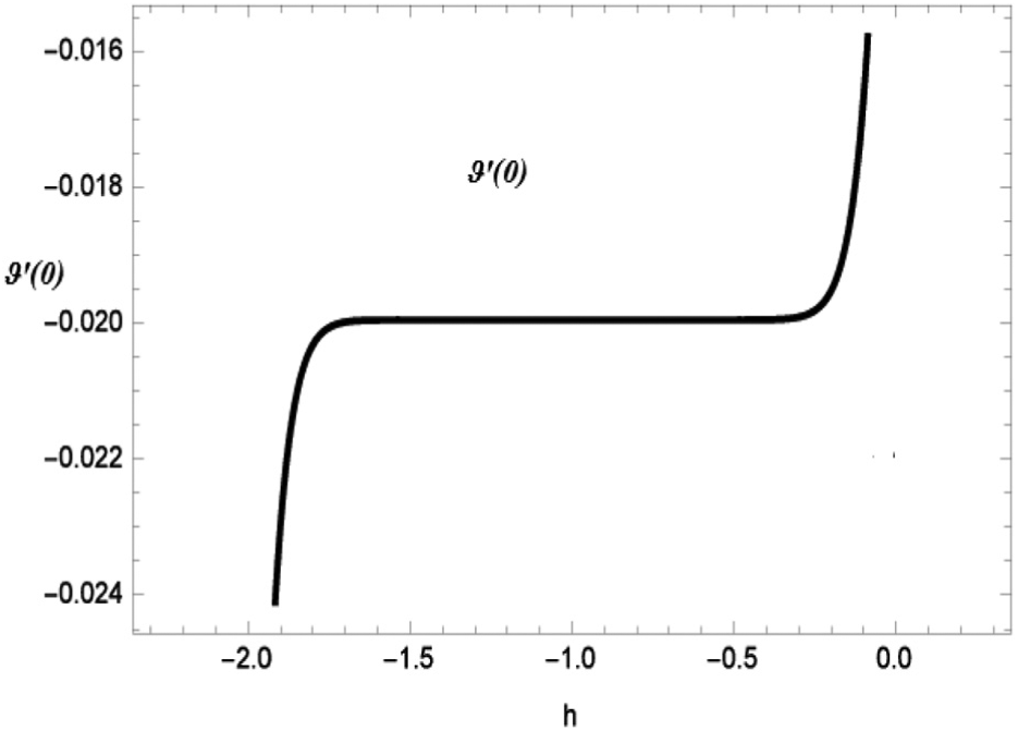
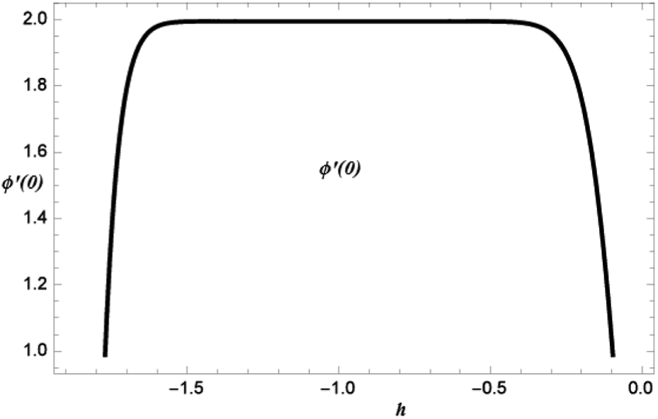
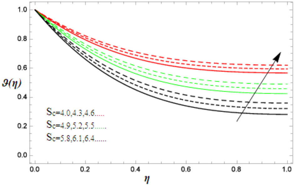
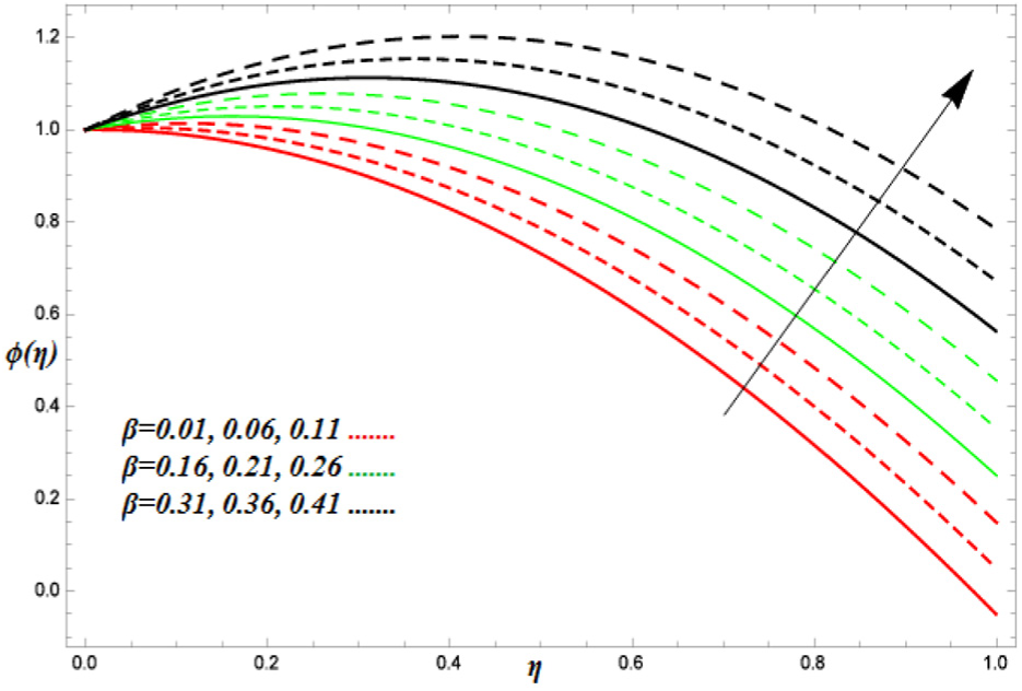
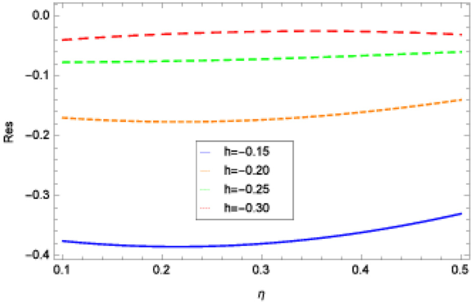
Figure 2 shows the h-curve region for velocity field. It is shown that the valid region for $f″(0)$ is $-3.3<h<-0.5$ . Figure 3 shows the h-curve region for temperature field. It is presented that the valid region for $\vartheta \prime (0)$ is $-1.9<h<-0.1$ . Figure 4 shows the h-curve region for velocity, temperature, and concentration fields. It is shown that the valid region for $\varphi \prime (0)$ is $-1.8<h<-0.2$ . The variable viscosity parameter $\mathrm{\Lambda }$ shows important part in the motion which is shown in Figure 5. The cohesive and adhesive forces have directly proportion to viscosity. Therefore, increase in $\mathrm{\Lambda }$ generating strong, cohesive, and adhesive forces, present resistance, which reduce generally fluid motion. In Figure 6, the character of viscosity parameter $\mathrm{\Lambda }$ is displayed; an increase in the viscosity parameter rises the viscous forces that is why the fluid becomes thicker and thereby reduces the temperature. In other words, viscosity parameter $\mathrm{\Lambda }$ has an inverse relation with temperature. That is, the increase of the viscosity factor $\mathrm{\Lambda }$ causes decrease in the thermal boundary coating wideness which consequences decrease in the temperature. The velocity distribution for several values of Prandtl number $\mathrm{Pr}$ is demonstrated in Figure 7. It is shown that rising values of $\mathrm{Pr}$ decrease the boundary layer size, subsequently reduces the velocity. Physically, the Prandtl number is a dimensionless quantity and is the ratio of kinematic viscidness to thermal diffusivity. When the value of momentum diffusivity is greater than the thermal diffusivity, the value of Prandtl quantity increased. Thus, heat transmission at the surface growths with increasing quantity of the Prandtl number while the mass transmission is concentrated with the increase in Prandtl number. The effect of Prandtl number $\mathrm{Pr}$ has been shown in Figure 8, defining that $\vartheta (\eta )$ reduces with larger values of $\mathrm{Pr}$ . The reason is that with the greater values of Prandtl quantity, the thermal boundary layer reduces. The consequence is even more obvious for slight Prandtl number since the thermal boundary layer thickness is relatively great. It is clear that an increase in the Prandtl number drops the temperature profiles of the flow. This is due to the fact that with the increase in the Prandtl number causes to increase the viscosity of the fluid, which causes to improve the wall friction along with the thermal conductivity. Due to this reason, we have seen a fall in the temperature profiles of the flow. In case of Figure 9, concentration field illustrates a reducing behavior against Prandtl number $\mathrm{Pr}$ due to the thinning of the boundary layer. Figure 10 displays that by changing the Schmidt number $S_c$ , the non-dimensional temperature profile $\vartheta (\eta )$ increases. Figure 11 displays that for dissimilar measures of Schmidt parameter $S_c$ , the non-dimensional concentration profile $\varphi (\eta )$ drops. It is clear that a flow of fluid rises in the parallel direction by giving rise into the Schmidt number. As Schmidt parameter is the ratio of momentum and concentration diffusivities and increase in $S_c$ , decreases the thickness of the fluid and consequently $\varphi (\eta )$ drops. It is imperative for higher quantities of Schmidt numbers, the viscous dissipation effects on the particle volume fraction are insignificant. From Figure 12, it seems that the velocity sketch reductions with greater values of film thickness constraint $\beta$ fluid film resistance to the flow and slow down the fluid velocity. $\vartheta (\eta )$ decreases with larger values of $\beta$ which is observable in Figure 13. Heat is absorbed in the fluid film size; therefore, temperature reduces. The concentration profile $\varphi (\eta )$ rises up with growing values as exhibited by Figure 14.The purpose is that the film thickness has direct proportion to viscosity and thermal conductivity. Figure 15 is prepared for the magnetic field constraint $M$ . As the values of magnetic parameter increase on the plate surface with thermal radiation and thermophoresis throughout the flow, the flow rate reduces which results the reduction of the velocity profiles as shown in Figure 15. Commonly, the momentum boundary layer develops thin with larger values of $M$ . The reason for that is the implementation of magnetic field to a fluid produces a resistance force named the Lorentz force, which is accountable to bring the retardation in the movement of the fluid. It is also detected that Jeffrey fluid is remarkably affected by the Lorentz’s force as compared to Maxwell and Oldroyd-B fluids. The magnetic field constraint $M$ increases with temperature and with growing values of $M$ as established by Figure 16. It is distinguished that the heat of the fluid rises for larger values of $M$ attached to the surface of the plate and the effect is not projecting far-away from the plate. Figure 17 labels that concentration field is growing with several values of magnetic parameter $M$ . The purpose is that by increasing magnetic field on the fluid gives increase to a Lorentz force. This force is like to drag force which is developed near the channel walls and inferior in the middle of the channel and at the boundaries. Velocity increases with the unsteady parameter S. From Figure 18, it is clear that all the three fluids show the same reaction to the unsteady parameter. The steepness in the temperature profiles decreases, reducing the thicknesses of the thermal boundary layers. The unsteady parameter $S$ has opposite effect on temperature profile. Figure 19 shows that temperature decreases with the unsteady parameter $S$ . Each and every fluid has the similar effect on temperature for the unsteady parameter $S$ . The Brownian motion constraint increases with the free surface temperature, as shown in Figure 20. The fact is that the arbitrary motion of the particles of the fluid generates the collision of the particles. By increasing the value of Brownian motion constraint $N_b$ , the heat in the fluid increases, consequences the reduction of the free surface particle volume fraction and which is displayed in Figure 21. The thermophoresis parameter $N_t$ faces decrease in contrast with temperature profile. This phenomenon is described by Figure 22. The thermophoresis limitation supports the growth in surface temperature. The irregular moment of suspended particles in fluid represents the Brownian motion. Due to this irregular motion, suspended, particles produce kinetic energy and the temperature increases and as a result, the thermophoretic force produces a flow away from the stretching sheet and the more intense fluid is moved away from the surface, and subsequently, as $N_t$ grows, the temperature inside the boundary layer rises. With the increasing values of thermophoresis parameter $N_t$ , elevation occurs in the concentration profile. Figure 23 shows that thermophoresis restriction also helps in rising the surface particle volume fraction like the surface temperature. Increasing the thermophoresis parameter $N_t$ will decrease surface mass transfer rate in each of the steady and unsteady cases, but showing high surface mass transfer rate in unsteady than steady case. The comparison between HAM and numerical solution has been displayed in Figures 24–26 for velocity, temperature, and concentration profiles, respectively. Figures 27–29 indicate h curves of the residuals for velocity, temperature, and concentration profiles, respectively. In most of the existing literature, the parameter range is avoided and the convergence is only dependent on the h curves. The parameter range is very necessary and plays a vital role to achieve the prominence convergence. The residual error and parameter range have been examined for the velocity, temperature, and concentration fields to authenticate the HAM solution in Figures 30 and 31. Table 1 has been designed to show the contribution of the present work in the existing literature. The numerical comparison and absolute errors of these profiles have been plotted in Tables 2–4. The convergence of the solution is shown in Table 5 and it is observed that momentum equation converges to 20th order of approximations whereas temperature distribution equation converges at 24th order of approximations and concentration equation converges up to 24th order of approximations. The skin friction with changing controlling parameters at the boundaries has been defined in Table 6. From Table 6, the characteristic behavior of $S,\mathrm{\Lambda },M$ , and $\mathrm{Pr}$ on the skin friction is demonstrated. It is noted from the table that higher degrees of skin friction are obtained for increasing values of $\mathrm{\Lambda }$ and $M$ while the reverse is the case for $S$ and $\mathrm{Pr}$ . The Nusselt number with changing controlling parameters at the boundaries has been defined in Table 7. From Table 7, the characteristic behavior of $S,\mathrm{Pr},N_t$ , and $N_b$ on the Nusselt number is demonstrated. It is noted from the table that it increased with increasing values of $S$ and $\mathrm{Pr}$ while the reverse affects the case for $N_t$ and $N_b$ . The Sherwood number with changing controlling parameters at the boundaries has been defined in Table 8. The characteristic behavior of $S,N_b,N_t$ , and $S_c$ on the Sherwood number is demonstrated. It is noted from the table that Sherwood number increased with increasing values of $N_b$ and $S_c$ while the reverse affects in case for $S$ and $N_t$ .

Figure 24.

Comparison of HAM and numerical results for $f\prime (\eta )$ when $h=-0.2,{\delta }_1=0,{\delta }_2=0.5,{\delta }_3=0.5,S=0.9,{ϵ}_3=0.8,M=0.7,\mathrm{\Lambda }=0.5,\mathrm{Pr}=0.6,\epsilon =1,N_b=0.6,S_c=0.6,\beta =1,N_t=0.6$ .

Figure 25.

Comparison of HAM and numerical results for $\theta (\eta )$ when $h=-0.2,{\delta }_1=0,{\delta }_2=0.5,{\delta }_3=0.5,S=0.9,{ϵ}_3=0.8,M=0.7,\mathrm{\Lambda }=0.5,\mathrm{Pr}=0.6,\epsilon =1,N_b=0.6,S_c=0.6,\beta =1,N_t=0.6$ .

Figure 26.

Comparison of HAM and numerical results of $\varphi (\eta )$ when $h=-0.2,{\delta }_1=0,{\delta }_2=0.5,{\delta }_3=0.5,S=0.9,{ϵ}_3=0.8,M=0.7,\mathrm{\Lambda }=0.5,\mathrm{Pr}=0.6,\epsilon =1,N_b=0.6,S_c=0.6,\beta =1,N_t=0.6$ .

Figure 27.

Shows h curves of the residuals for the velocity profile $f(\eta )$ when $h=-0.2,{\delta }_1=0,{\delta }_2=0.5,{\delta }_3=0.5,S=0.9,{ϵ}_3=0.8,M=0.7,\mathrm{\Lambda }=0.5,\mathrm{Pr}=0.6,\epsilon =1,N_b=0.6,S_c=0.6,\beta =1,N_t=0.6$ .

Figure 28.

Shows h curves of the residuals for the temperature profile $\theta (\eta )$ when $h=-0.2,{\delta }_1=0,{\delta }_2=0.5,{\delta }_3=0.5,S=0.9,{ϵ}_3=0.8,M=0.7,\mathrm{\Lambda }=0.5,\mathrm{Pr}=0.6,\epsilon =1,N_b=0.6,S_c=0.6,\beta =1,N_t=0.6$ .

Figure 29.

Shows h curves of the residuals for the concentration profile $\varphi (\eta )$ when $h=-0.2,{\delta }_1=0,{\delta }_2=0.5,{\delta }_3=0.5,S=0.9,{ϵ}_3=0.8,M=0.7,\mathrm{\Lambda }=0.5,\mathrm{Pr}=0.6,\epsilon =1,N_b=0.6,S_c=0.6,\beta =1,N_t=0.6$ .

Figure 30.

Residual error for the parameter range $\mathrm{Pr}$ .

Figure 31.

Residual error sketch for the parameter range $S_c$ .

Table 1.

Collected works on non-Newtonian nano-liquid film on a stretching sheet.

Authors	Variable viscosity	Variable thermal conductivity	Non-Newtonian three fluids	Brownian diffusion constant	Thermophoretic diffusion constant
Sandeep et al.	Not considered	Not considered	Considered	Not considered	Not considered
Qasim et al. 10	Not considered	Not considered	Not considered	Considered	Considered
Abolbashari et al. 9	Considered	Considered	Williamson fluid	Not considered	Not considered
Present work	Considered	Considered	Considered	Considered	Considered

Table 2.

Shows the association between HAM and ND-Solve for velocity pitch $f\prime (\eta )$ when $h=-0.2,{\delta }_1=0,{\delta }_2=0.5,{\delta }_3=0.5,S=0.9,{ϵ}_3=0.8,M=0.7,\mathrm{\Lambda }=0.5,\mathrm{Pr}=0.6,\epsilon =1,N_b=0.6,S_c=0.6,\beta =1,N_t=0.6$ .

$\eta$	HAM solution $f\prime (\eta )$	Numerical solution NS	Absolute error	$\eta$	HAM solution $f\prime (\eta )$	Numerical solution NS	Absolute error
0	1.0000	1.0000	0.0	0.6	0.433323	0.431739	$1.6\times {10}^{-3}$
0.1	0.860215	0.865382	$4.8\times {10}^{-3}$	0.7	0.387843	0.388044	$2.0\times {10}^{-4}$
0.2	0.754546	0.748225	$6.3\times {10}^{-3}$	0.8	0.355835	0.357923	$2.1\times {10}^{-3}$
0.3	0.65306	0.647075	$5.9\times {10}^{-3}$	0.9	0.336946	0.34077	$3.8\times {10}^{-3}$
0.4	0.565754	0.560968	$4.8\times {10}^{-3}$	1	0.330755	0.335423	$4.7\times {10}^{-3}$
0.5	0.492556	0.489304	$3.3\times {10}^{-3}$

HAM: homotopy analysis method; NS: numerical solution.

Table 3.

The association between HAM and ND-Solve shown for $\theta (\eta )$ when $h=-0.2,{\delta }_1=0,{\delta }_2=0.5,{\delta }_3=0.5,S=0.9,{ϵ}_3=0.8,M=0.7,\mathrm{\Lambda }=0.5,\mathrm{Pr}=0.6,\epsilon =1,N_b=0.6,S_c=0.6,\beta =1,N_t=0.6$ .

$\eta$	HAM results of $\theta (\eta )$	Numerical results NS	Absolute error	$\eta$	HAM results of $\theta (\eta )$	Numericalresults NS	Absolute error
0	1.0000	1.00000	0.00000	0.6	0.762633	0.757494	$5.1\times {10}^{-3}$
0.1	0.937702	0.9303116	$7.4\times {10}^{-3}$	0.7	0.74749	0.744597	$2.9\times {10}^{-3}$
0.2	0.886216	0.875477	$1.1\times {10}^{-2}$	0.8	0.737235	0.736031	$1.2\times {10}^{-3}$
0.3	0.844103	0.832878	$1.2\times {10}^{-2}$	0.9	0.731369	0.73116	$2.1\times {10}^{-4}$
0.4	0.810135	0.800239	$9.9\times {10}^{-3}$	1	0.72949	0.729589	$9.9\times {10}^{-5}$
0.5	0.783271	0.775633	$7.6\times {10}^{-3}$

HAM: homotopy analysis method; NS: numerical solution.

Table 4.

The association between HAM and ND-Solve shown for $\phi (\eta )$ when $h=-0.2,{\delta }_1=0,{\delta }_2=0.5,{\delta }_3=0.5,S=0.9,{ϵ}_3=0.8,M=0.7,\mathrm{\Lambda }=0.5,\mathrm{Pr}=0.6,\epsilon =1,N_b=0.6,S_c=0.6,\beta =1,N_t=0.6$ .

$\eta$	HAM solution $\varphi (\eta )$	Numerical solution NS	Absolute error	$\eta$	HAM solution $\varphi (\eta )$	Numerical solution NS	Absolute error
0	1.00000	1.000000	0.000000	0.6	1.20063	1.20172	$1.1\times {10}^{-3}$
0.1	1.04865	1.05256	$3.9\times {10}^{-3}$	0.7	1.21532	1.21472	$6.0\times {10}^{-4}$
0.2	1.09068	1.09617	$5.5\times {10}^{-3}$	0.8	1.2255	1.2235	$2.0\times {10}^{-3}$
0.3	1.12653	1.13199	$5.5\times {10}^{-3}$	0.9	1.23144	1.22851	$2.9\times {10}^{-3}$
0.4	1.15656	1.161	$4.4\times {10}^{-3}$	1	1.23337	1.2301	$3.8\times {10}^{-3}$
0.5	1.18115	1.18401	$2.9\times {10}^{-3}$

HAM: homotopy analysis method; NS: numerical solution.

Table 5.

Shows the convergence of the HAM approximated solutions when $h=-.5,{\delta }_1=0.1,{\delta }_2=1.0,{\delta }_3=0.1,S=0.5,{ϵ}_3=0.1,M=0.6,\mathrm{\Lambda }=0.7,\mathrm{Pr}=1.0,\epsilon =0.5,N_b=0.6,S_c=0.6,\beta =1,N_t=1.0$ .

Order of approximations	$-f″(0)$	$-\vartheta \prime (0)$	$-\varphi \prime (0)$	Order of approximations	$-f″(0)$	$-\vartheta \prime (0)$	$-\varphi \prime (0)$
1	0.390500	0.412500	0.206250	20	0.703107	0.500542	−0.428239
5	0.688922	0.496720	−0.373811	24	0.703107	0.500543	−0.428246
10	0.702788	0.500338	−0.425435	25	0.703107	0.500543	−0.428246
15	0.703100	0.500532	−0.428099

HAM: homotopy analysis method.

Table 6.

Exhibits the numerical values for skin friction coefficient for several physical parameters when $h=-0.5,{\delta }_1=0.1,{\delta }_2=1.0,{\delta }_3=0.1,S=0.5,{ϵ}_3=0.1,M=0.6,\mathrm{\Lambda }=0.7,\mathrm{Pr}=1.0,\epsilon =0.5,N_b=0.6,S_c=0.6,\beta =1,N_t=1.0$ .

$S$	$\mathrm{\Lambda }$	$M$	$\mathrm{Pr}$	$-\frac{1+{\delta }_1}{1+{\delta }_2}f″(0)$	$S$	$\mathrm{\Lambda }$	$M$	$\mathrm{Pr}$	$-\frac{1+{\delta }_1}{1+{\delta }_2}f″(0)$
0.5	0.5	0.6	1.0	0.346659	0.5	0.5	0.6	1.0	0.386709
0.6	0.5	0.6	1.0	0.336475	0.5	0.5	0.7	1.0	0.388120
0.7	0.5	0.6	1.0	0.327884	0.5	0.5	0.8	1.0	0.389529
0.5	0.5	0.6	1.0	0.346659	0.5	0.5	0.6	1.0	0.386709
0.5	0.6	0.6	1.0	0.366769	0.5	0.5	0.6	1.1	0.386289
0.5	0.7	0.6	1.0	0.386709	0.5	0.5	0.6	1.2	0.385895

Table 7.

Exhibits the numerical values of local Nusselt number for several physical parameters when $h=-0.5,{\delta }_1=0.1,{\delta }_2=1.0,{\delta }_3=0.1,S=0.5,{ϵ}_3=0.1,M=0.6,\mathrm{\Lambda }=0.7,\mathrm{Pr}=1.0,\epsilon =0.5,N_b=0.6,S_c=0.6,\beta =1,N_t=1.0$ .

$S$	$\mathrm{Pr}$	$N_t$	$N_b$	$-(1+\epsilon \vartheta (0))\vartheta \prime (0)$	$S$	$\mathrm{Pr}$	$N_t$	$N_b$	$-(1+\epsilon \vartheta (0))\vartheta \prime (0)$
0.5	1.0	1.0	0.6	0.754569	0.5	1.0	1.0	0.6	0.750815
0.6	1.0	1.0	0.6	0.795885	0.5	1.0	1.1	0.6	0.750720
0.7	1.0	1.0	0.6	0.836769	0.5	1.0	1.2	0.6	0.750626
0.5	1.0	1.0	0.6	0.750815	0.5	1.0	1.0	0.6	0.750815
0.5	1.1	1.0	0.6	0.797904	0.5	1.0	1.0	0.7	0.749006
0.5	1.2	1.0	0.6	0.841992	0.5	1.0	1.0	0.8	0.747203

Table 8.

Exhibits the numerical values of local Sherwood number for several physical parameters when $h=-0.5,{\delta }_1=0.1,{\delta }_2=1.0,{\delta }_3=0.1,S=0.5,{ϵ}_3=0.1,M=0.6,\mathrm{\Lambda }=0.7,\mathrm{Pr}=1.0,\epsilon =0.5,N_b=0.6,S_c=0.6,\beta =1,N_t=1.0$ .

$S$	$N_t$	$N_b$	$S_c$	$-\varphi \prime (0)$	$S$	$N_t$	$N_b$	$S_c$	$-\varphi \prime (0)$
0.5	1.0	0.6	0.5	−0.430156	0.5	1.0	0.6	0.5	−0.428246
0.6	1.0	0.6	0.5	−0.451157	0.5	1.0	0.7	0.5	−0.311183
0.7	1.0	0.6	0.5	−0.471662	0.5	1.0	0.8	0.5	−0.223390
0.5	1.0	0.6	0.5	−0.428246	0.5	1.0	0.6	0.5	−0.428246
0.5	1.1	0.6	0.5	−0.508897	0.5	1.0	0.6	0.6	−0.347718
0.5	1.2	0.6	0.5	−0.589527	0.5	1.0	0.6	0.7	−0.268237

Conclusion

Regarding to various applications in engineering and industrial apparatus of the study, we extend a mathematical model for studying the liquid film flow of non-Newtonian fluids with variable viscosity and thermal conductivity in the presence of a magnetic field. The model of the flow is considered for Jeffrey, Maxwell, and Oldroyd-B fluids over a stretched surface. The obtained highly coupled non-linear equation has been solved using HAM and numerical (ND solve) methods. We powerfully trust that this revision provides a worthy possibility to the investigators to classify the high thermal conductivity, non-Newtonian fluid which provides good heat transfer equipment for high thermal conductive nanoparticles.

The key concluded remarks of this work are as follows:

1. The variable viscosity and thermal conductivity effects on the flow of Jeffrey, Maxwell, and Oldroyd-B fluids are discussed through graphs and tables.

2. It is also concluded that Jeffrey fluid is remarkably affected by the Lorentz’s force as compared to Maxwell and Oldroyd-B fluids.

3. Non-dimensional velocity reduction in variable viscosity and magnetic constraints.

4. The temperature and concentration fields both are directly related to magnetic fields.

5. Rising the particle concentration efficiently increases the friction features of Jeffrey, Maxwell, and Oldroyd-B fluids.

6. Lorentz force efficiently controls the momentum boundary layer of Jeffrey fluid. Lorentz force capably reduces the momentum boundary layer and increases the thermal boundary layer thickness. It is remarkable to mention here that the Jeffrey fluid is highly effective by magnetic field parameter compared with other two fluids.

7. The effect of Prandtl number on the temperature profiles has inverse relation.

8. This study is very valuable for scheming the heat exchanger apparatus.

9. The confirmation of the obtained solution through HAM has been verified by numerical methods.