Sage Journals: Discover world-class research

Abstract

A test platform with a millimeter-wave radar sensor, lane-line sensor, gyroscope, and controller area network was established to improve safety in using adaptive cruise control systems in vehicles. The motion-state characterization data of the host vehicle and surrounding vehicles in a real traffic environment were captured. The prediction method for the lane-changing maneuver of the vehicle ahead was developed using a hidden Markov model based on the distance between the host vehicle and the front vehicle, as well as the lateral and longitudinal velocities of the vehicle in front. The adaptive cruise control system control algorithm for assessing the target vehicle was optimized. The model was tested, and its predictions were compared with measured data. Result shows that the lane-changing and lane-keeping behaviors of the vehicle ahead can be predicted efficiently and accurately by the model. The maximum prediction accuracy rate for straight roads was 97% with the time window length of 4.5 s, whereas that for curved roads was 96% with the time window length of 3.5 s.

Keywords

Vehicle lane change prediction adaptive cruise control hidden Markov model

Introduction

Adaptive cruise control (ACC) systems help drivers to control their vehicles conveniently and safely, and these systems fill in a significant part in promoting the development of conventional vehicles to unmanned vehicles. The ACC system adjusts the speed of the host vehicle to ensure car-following safety in real time according to the speed of surrounding vehicles. It often occurs, in car-following state, that the preceding vehicle quickly changes lane or another vehicle suddenly cut in front the host vehicle. In this case, an ACC system frequently changes its tracking target, causing the frequent sudden acceleration–deceleration switches, which tremendously affects driving safety and comfort.¹ Therefore, if the motion state of the vehicle ahead can be predicted in advance, the ACC system can respond to a sudden switch in the motion states of the vehicle ahead in advance; as a result, a safe following distance is maintained, and driving safety is ultimately ensured.

Currently, numerous studies focused on lane-change prediction of host vehicle. Many studies have been interested in understanding driver’s intent via their visual behaviors and head motion, which can be used to predict the lane-change maneuvers of host vehicle. Morris et al.² used head motion, relative speed and distance between surrounding vehicles and host vehicle to continuously predict lane changes. A Doshi and Trivedi³ considered the eye gaze behavior of the driver as a predictive feature to identify lane-keeping and lane-change behaviors. Visual search behaviors and time-to-collision (TTC) can be used to predict drivers’ lane-change behavior with back-propagation (BP) neural network.⁴ GM Fitch et al.⁵ divided the monitoring area into eight categories, proposed a time window of 3.0 s and detected lane-change intention by studying the gaze behavior characteristics of the driver before changing lanes at different time points. W Yuan et al.⁶ captured the eye movement data of drivers and established a lane-change intention identification method by multi-evidence fusion identification. These studies proposed an understanding of the driver’s intent by utilizing an eye and head motion tracking system; thus, the prediction accuracy relied heavily on the patterns of visual search (eye and head motion) and it can be easily affected by light intensity.

Lane-change intent can be identified based on vehicle motion parameters before lane-change maneuver. Dogan et al.⁷ carried out experiments in the driving simulator and proposed a driver cognitive model of lane change based on the information of lane offset, lateral acceleration, and steering angle. Using support vector machine, lane-change intention can be predicted with respect to lane information, speed, and steering angle.⁸ Based on the adaptive fuzzy pattern classification, F Bocklisch et al.⁹ proposed a prediction method for the lane-change intention of the host vehicle. Based on the information of lane position, vehicle motion parameters, and head motion, JC McCall et al.¹⁰ established an intention–recognition model for high-speed driving with sparse Bayesian learning. H Zhou et al.¹¹ proposed a method to infer a truck driver’s intention of lane change before the maneuver initiation using the information of driver’s gaze behavior. C Ding et al.¹² provided a method to predict the lane-change trajectory of host vehicle with regard to the vehicle position, speed, acceleration, and the time headway using BP neural network with two hidden layers. Furthermore, host vehicle trajectory can be predicted with the positional relationship between the host vehicle and adjacent vehicles.¹³ Tang et al.¹⁴ conducted driving experiments at different speeds in the driving simulator and proposed a prediction model based on the adaptive fuzzy neural network.

Relatively less research focused on lane-change intention prediction of surrounding vehicle. In prior intent prediction research,^15,16 vehicle-to-vehicle communication has been considered as an effective approach to analyze the motion of surrounding vehicle; most of these studies were conducted in the simulator and cannot be applied in real road without communication tools. In addition, vision-based systems have been widely applied to the area of object detection and motion prediction,^17–19 such as the eye and head motion tracking system; however, it was vulnerable to weather. To overcome these obstacles, a radar-based vehicle motion prediction method has been developed, and the motion information of surrounding vehicle can be detected by millimeter-wave radar or lidar. In the work by Kajiwara,²⁰ the following and oncoming vehicle’s path can be estimated based on heading angle of the vehicle and the curvature of road, which can provide host vehicle a safe stop position. Based on multilayer perceptron approach, Yoon and Kum²¹ proposed a lateral motion prediction method using lateral position of surrounding vehicle. Liu et al.²² developed an estimation and classification model of traffic accidents risk based on hidden Markov models (HMMs) with respect to the yaw angle and width of surrounding vehicle. Although these literature have focused on the impact of lane change on the traffic accidents, the influence of driving behavior on ACC is relatively understudied.

In this article, we use the HMM, which is widely used in state and lane-change intention prediction, to optimize the control algorithm for ACC systems.^23–26 The proposed prediction algorithm can be used in both straight road and curved road. The remainder of this article is composed as follows. Section “Prediction model” introduces the details of our algorithm. Section “Model testing and training” shows model testing and training. A conclusion of the work is given in section “Conclusion.”

Prediction model

HMM

Generally, lane change can be divided into the following stages: preparation stage, initiating change stage, continuously changing stage, and end stage. Characterization parameters were used to classify these stages, including the horizontal distance to lane line and horizontal and vertical vehicle speeds. In the surface layer, the division of the stages is determined by changes in the characterization parameters; however, the motion state of a vehicle cannot be generated suddenly. Within a sequence of events, a switching between states is probable. The HMM can handle this mechanism between states; it is a common forecasting tool in the field of pattern recognition. The prediction process is commonly based on the existing state to forecast the next stage condition. Thus, we can apply this model. We first determine and analyzing the lane-change intention and characterization parameters of the front vehicle. We then identify the underlying law and apply this to analyze and forecast the lane-change intention of the preceding vehicle.^27,28

The HMM is an extension of the visible Markov model. It is a probabilistic model used to describe the statistical properties of a random process represented by parameters; this model is a doubly stochastic process. It consists of Markov chains and general stochastic processes, as shown in Figure 1.

Figure 1.

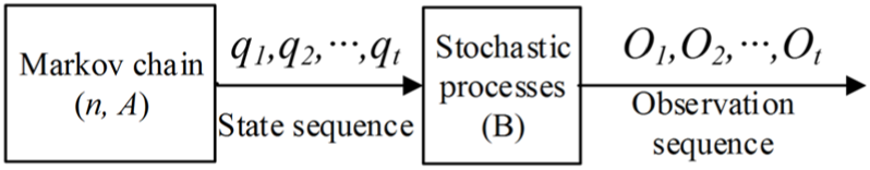
Composition of a hidden Markov chain.

The HMM is defined as follows:

X represents the hidden state set, X = {X₁, X₂, …, X_N}, where N represents the number of states; Q = {q₁, q₂, …, q_T}, q_t represents the hidden state at the t moment.

V represents the observation set, V = {V₁, V₂, …, V_M}, where M is the number of different observed values from each state. O represents the observation sequence set, O = {O₁, O₂, …, O_T}, O_t represents the observation state at the t moment.

The state transition probability matrix A = {a_ij}, where a_ij = P{q_t_+ 1 = X_j − q_t = X_i}, $1 ⩽ i, j ⩽ N$ .

The state j observation probability matrix $B = {b_{j} (k)}$ represents the probability of the corresponding observed value of the state j output, where in b_j(k) = P{O_t = V_k − q_t = X_j}, $1 ⩽ j ⩽ N, 1 ⩽ k ⩽ M$ . Given the continuity of the model parameters, a continuous probability density function is used to represent the observation probability

b_{j} (O) = \sum_{m = 1}^{M} c_{j m} N (O, μ_{j m}, U_{j m})

(1)

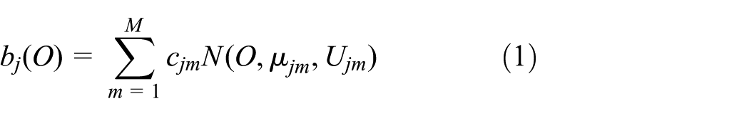
where O is the observation sequence to be fitted, and $c_{jm}$ , $μ_{jm}$ , and $U_{jm}$ are the mixed weights, mean vectors, and covariance matrices of the mixed functions m for the state $X_{j}$ , respectively.

5. The initial state distribution is $π = {π_{i}}, π_{i} = P {q_{1} = X_{i}}, 1 ⩽ i ⩽ N$ .

Therefore, the HMM can be expressed as a 5-tuple: $λ = (X, O, A, B, π)$ .

In accordance with the HMM, the lane-change motion state of the preceding vehicle is derived as follows:

$X = (X_{1}, X_{2}, X_{3})$ , where $X_{1}$ represents lane keeping, $X_{2}$ represents left lane changing, and $X_{3}$ represents right lane changing.

$O = (O_{1}, O_{2}, \dots, O_{i} \dots, O_{n})$ , where $O_{i} = f (d, V_{x}, V_{y})$ . The lateral distance between the lane and the vehicle in front is represented by d (cm); the lateral velocity of the front vehicle is represented by $V_{x}$ (km/h); the longitudinal velocity of the vehicle ahead is represented by $V_{y}$ (km/h).

The motion-state transition probability matrix of the front vehicle is $A = (a_{ij})_{3 \times 3}$ , where $a_{ij}$ represents the probability of the motion-state transition of the vehicle ahead.

$B = (b_{j})_{3 \times n}$ , where $b_{j}$ represents the probability of the observation set O of the vehicle ahead under the condition X.

The initial state distribution is represented by $π$ .

Given that driving is a continuous process and the current state only depends on the previous state based on the continuity of the vehicle-operating parameters, the left-to-right chain structure is selected, and the number of hidden states in each intention model is set to 3, and the Gauss mixture number is 3. The left-to-right chain structure of the HMM is shown in Figure 2.

Figure 2.

Left-to-right chain structure of hidden Markov model.

Prediction model for straight section

Figure 3 shows that the host vehicle H and front vehicle F are in a straight section. H drives in lane 1, and F drives in lane 2. Lane width is denoted by W; the distances between the host car and the left and right lanes are d_L and d_R; and the distance, lateral distance, and angle between H and F are denoted by r, D, and α, respectively. The distance between F and the left lane is d, and the lateral and longitudinal speeds are V_x and V_y.

Figure 3.

Relationship in straight section.

Among the aforementioned parameters, the parameters that can directly indicate lane-change intention of the front vehicle F are d, V_x, and V_y. Among these parameters, the characterization of d is the most significant. In terms of the cooperative interaction mechanism of vehicle-road parameters, parameter d changes according to a certain rule in the lane-changing process, and this change process directly reflects the lane-change intention of vehicle F. After the start of the lane change, the lateral speed of the front vehicle F presents certain characteristics different from the lateral speed caused by the sway of the vehicle body in normal-course driving. Consequently, the parameter V_y will also increase or decrease. On the basis of the given analysis, d, V_x, and V_y are used as the characterization parameters in the prediction model for the lane-change intention of F in straight sections.²⁹

Prediction model for curved road

Unlike in the straight section, parameter d in the curved section cannot be directly obtained because of the influence of road curvature. Therefore, to the curvature of the intermediate parameters must first be measured to obtain the value of d and establish the prediction model for the curved section. Road curvature can be calculated by vehicle speed and yaw rate

C = \frac{ω}{v} = \frac{1}{R}

(2)

where C is road curvature 1/m; v is vehicle circumferential motion speed, m/s; $ω$ is the yaw rate measured by the vehicle gyroscope, rad/s; R is the curvature radius of the road, m.

Figure 4 shows that the host vehicle H and front vehicle F are in a curved section. The circumferential motion speed v can be calculated by $v = R \times β / t$ , where $β$ is the central angle for vehicles corresponding to the arc length in t time. In the prediction model for the curved section, d, V_x, and V_y are used to predict the lane-change intention of the front vehicle F.

Figure 4.

Relationship between vehicles on curved road.

Parameter acquisition and filtering

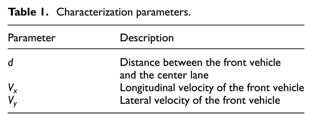
For the actual road test, we selected common vehicles as test instruments and equipped them with a vehicle radar sensor, lane-detection sensors, an on-board gyroscope, vehicle controller area network (CAN) bus, and data acquisition equipment. The motion states of the host vehicle and the vehicle ahead and the road traffic environment information are acquired. Table 1 shows the characterization parameters of prediction model.³⁰

Table 1.

Characterization parameters.

Parameter	Description
d	Distance between the front vehicle and the center lane
V_x	Longitudinal velocity of the front vehicle
V_y	Lateral velocity of the front vehicle

Using the parameters of the prediction models for the straight and curved roads, as, respectively, illustrated in Figures 3 and 4, we design a real-time online data storage module with a data storage frequency of 10 Hz. Parameters r and α reflect the position relation between the host vehicle and the front vehicle and are measured by the radar sensor. The effective measurement range of the radar is 200 m and its measurement angle is 90°. Parameters d_L and d_R are measured by a lane-line identification sensor, whose measurement accuracy is 5 cm. The speed of the host vehicle is derived from the vehicle’s CAN bus, whose measurement accuracy is 0.01 km/h. The yaw rate data are generated by the on-board gyroscope, whose measurement accuracy is 0.1°/s. The parameters needed for the prediction models can be measured directly or indirectly with the data acquisition equipment.

In Figures 3 and 4, the speed of the vehicle H comes from the CAN bus, the speed of front vehicle F can be derived by superposition calculation with the speed of vehicle H, and the relative velocity is measured by the radar. The vector decomposition principle is used to derive the velocity components V_x and V_y of the front vehicle F. During the experiment, the output raw data measured by the sensors exhibit certain noises. Thus, before training, the raw measurement data must be filtered to reduce the noise and improve the potential connection characteristics of the internal data, as well as ensure the effectiveness and accuracy of the hidden Markov prediction model.

Kalman filtering is a filtering method often used in the field of pattern recognition. In the MATLAB environment, the Kalman filter is used to filter the original measurement data. The filtering effects of the Kalman filter on distance from lane line and speed are shown in Figures 5 and 6, respectively.

Figure 5.

Filtering result for distance to lane.

Figure 6.

Filtering result for speed.

Model testing and training

Optimal time window and model training

In a normal driving process, the motion state of vehicle F is divided into two, lane keeping and lane changing, which is divided into the left lane changing and right lane changing. Combined with the hidden Markov prediction model, in a certain time period, the motion states of the vehicle are lane keeping, left lane changing, or right lane changing. The training of the model is as follows:

Initialization: the state transition matrix A and mixed weight vector $c_{jm}$ are initialized to a random matrix. The mean vector $μ_{jm}$ and the covariance matrix $U_{jm}$ are initialized to the mean and covariance of the entire set of samples (M = 1) or a part of the sample (M ⩾ 2) corresponding to a certain state.

Using the current sample and the forward and backward algorithm, the forward probability $α_{t} (i)$ and backward probability $β_{t} (j)$ are calculated. The generated part of the observation sequence $O_{1}, O_{2}, \dots, O_{t}$ under the model $λ$ until the moment t and the probability of the state $X_{i}$ at time t are expressed by $α_{t} (i) = P (O_{1} O_{2}, \dots, O_{t}, q_{t} = X_{i} / λ)$ , $α_{t} (i)$ . The probability of the state $X_{i}$ at time t and the generated part of the observation sequence $O_{t + 1}, O_{t + 2}, \dots, O_{T}$ under the model $λ$ until the moment t are expressed by $β_{t} (i) = P (O_{t + 1} O_{t + 2}, \dots, O_{T}, q_{t} = X_{i} / λ)$ , $β_{t} (i)$ .

Calculate the current new model using the estimated values $\hat{λ} = (π, A, C_{jm}, μ_{jm}, U_{jm})$ .

Calculate the likelihood probability $P (O / \hat{λ})$ .

If $P (O / \hat{λ})$ is incremental, the new estimated value is used in step 3 for the estimates for the next time moment of the sample. Afterward, the procedure returns to step 2 iteratively until $P (O / \hat{λ})$ no longer significantly increases. Model $\hat{λ}$ is the solution model.

According to the aforementioned procedure, the training samples are selected, and the distance between the front car and the lane line, the front vehicle longitudinal velocity, and lateral velocity comprise the observation sequence $O (t) = {d (t), V_{x} (t), V_{y} (t)}$ where $d (t)$ is the distance between the car and lane at any time, $V_{x} (t)$ is the vehicle longitudinal velocity at any time, and $V_{y} (t)$ is the vehicle lateral velocity at any time.

The data on lane keeping and lane changing are selected from the front vehicle’s motion state data obtained from the actual road-driving test. Among them, 648 groups of the data are used for model training, and 216 groups are used for the model validity test. In the training process, a time window of 1.0 s is continuously identified, and the time interval for each data movement is set to 0.1 s. Tag attributes of the training samples are set. Therefore, by training the different motion states of the front vehicle F, the HMM can be used for continual analysis to determine the potential relationship between the internal characteristics of the data and the property tag. The data training process is shown in Figure 7.

Figure 7.

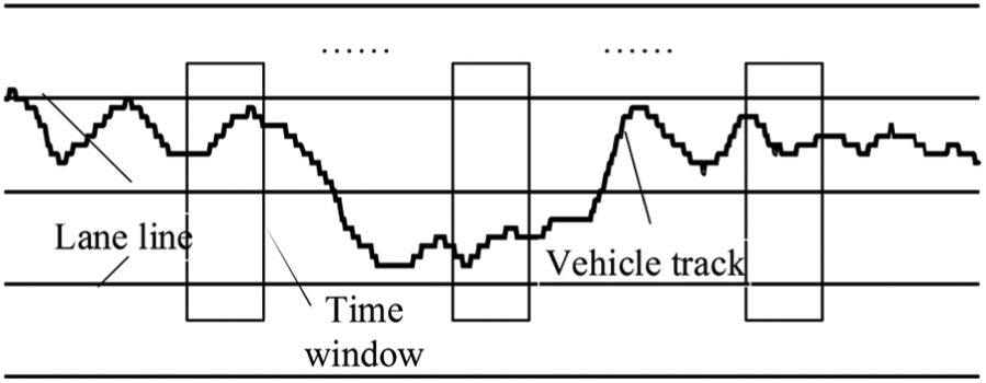
Moving time window.

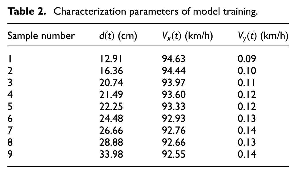
With the left lane changing as the example, Table 2 shows the characterization parameters of model training. After model training, the validity of the model is tested using the measured data. The result of the model is the state with the highest probability. If the probability value is close to 1, then the probability of the vehicle in the corresponding state is higher in the next time window. For a complete lane-changing behavior, 1.0 s is used as the length of the prediction time window. Table 3 shows the model prediction results.³¹

Table 2.

Characterization parameters of model training.

Sample number	$d (t)$ (cm)	$V_{x} (t)$ (km/h)	$V_{y} (t)$ (km/h)
1	12.91	94.63	0.09
2	16.36	94.44	0.10
3	20.74	93.97	0.11
4	21.49	93.60	0.12
5	22.25	93.33	0.12
6	24.48	92.93	0.13
7	26.66	92.76	0.14
8	28.88	92.66	0.13
9	33.98	92.55	0.14

Table 3.

Model predictions.

	L_K	L_CL	L_CR
Forecast probability	0.86	0.53	0.14
Forecast result	L_K

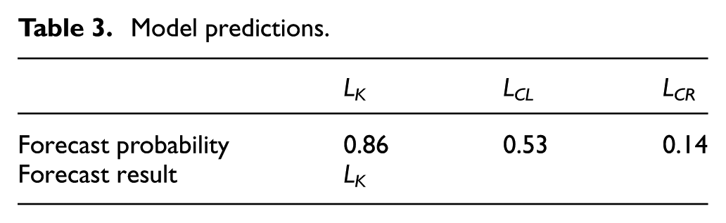
In Table 3, L_K denotes lane keeping, L_CL denotes the left lane changing, and L_CR indicates the right lane changing. In the corresponding time period in Table 3, the probability of the front vehicle in the next time the window being in the lane keeping state is 0.86, much higher than the left and right lane changing probability. Thus, the predicted result of the model is the lane-keeping state.

Aside from predicting accuracy, real-time prediction capability is an important factor in assessing the applicability of the model. For a time series, the longer the time window is, the larger the amount of data is; consequently, the prediction accuracy of the model will be higher. However, if the time window is extremely long, the potential data characteristics will be degraded, and the real-time prediction performance will be poor; therefore, extremely long time window is detrimental to the real-time requirements of the ACC system and other systems. Therefore, by analyzing and comparing the forecasting effects for different length time windows, the model can effectively meet the accuracy and real-time prediction requirements for ACC and other systems. With a time window length of 1.0 s, the model can identify the different vehicle motion states. Figure 8 shows the changes in the characterization parameters.

Figure 8.

Changes in the characterization parameters for different vehicle motion: (a) distance to lane, (b) lateral velocity, and(c) longitudinal velocity.

Considering the significant differences in the methods of identifying the positions between the straight and the curved sections, these two sections are separated in the model training and testing processes. In the interval of 0.5–5.0 s, using 0.5 s as the interval, the validity of the model is tested using different time window lengths, and the results are shown in Table 4.

Table 4.

Prediction accuracy of different time windows.

Time window		0.5	1.0	1.5	2.0	2.5	3.0	3.5	4.0	4.5	5.0
Forecast accuracy (%)	Straight section	70	73	77	84	88	90	95	96	97	95
Forecast accuracy (%)	Curved section	50	65	73	87	91	94	96	95	95	94

Table 4 shows the prediction accuracy rates for the straight and curved sections increase with an increase in the length of the time window. When the time window reaches 3.0 s, the prediction accuracy rates for the straight and curved sections are higher than 90%. As the time window length increases continually, the prediction accuracy continues to increase. When a certain peak is reached, the prediction accuracy rates for both sections begin to decline. For the straight section, when the time window length is 4.5 s, the prediction accuracy reaches the maximum value of 97%. For the curved section, when the time window length is 3.5 s, the prediction accuracy reaches the maximum value of 96%. If the time window is considerably short, the internal characteristics of the data are insufficient to characterize the motion state of the vehicle; thus, the model prediction accuracy is low. However, when the time window is considerably long, the potential law underlying the motion state of the vehicle can be affected by useless characterization data; thus, the prediction accuracy is reduced to a certain extent.

Forecast effect

In studying the predictive properties of the models further, we use the optimal time window lengths to predict the effects of the time window lengths on the accuracy of the models for the straight and curved sections. In the straight sections, the time window length adopted is 4.5 s. Thus, starting from 4.5 s before the lane-change starting point, with 0.1 s as the unit, the time window slides from left to right to obtain the lane-change time of vehicle F. Figure 9 shows the results of prediction process.

Figure 9.

Time ahead in straight section.

As shown in Figure 9, at 4.5 s before the lane-change starting point, the HMM predicts the lane-change intention of the front vehicle. Before a lane change, the prediction accuracy rates of the models are low. However, after passing the time window to the right, when the time window allows for sufficient data to characterize the state, the model can output a tag status value of a higher probability. As shown in Figure 9, from the lane-change starting point, 1.2 s after moving to the right, the model predicts correctly the lane-changing behavior.

For the curved section, the time window length is 3.5 s, and the same processing method is applied to the curved section. The prediction accuracy trend of the model is shown in Figure 10.

Figure 10.

Prediction effects of model in curved section.

Figure 10 shows that the result is similar to straight section calculated from the lane-change starting point; at 1.0 s after passing the time window to the right, the model output state tag value is predicted more accurately. Compared with the 1.2 s prediction time for straight sections, the prediction time for the curved sections is faster. This result may be attributed to the fact that in straight sections, the vehicle speed is usually faster than that in curved sections of the road. In similar scenarios, the data characteristics for straight sections are less than those for the curved sections; thus, the time required to predict lane change is longer for straight sections than for curved sections.³²

Conclusion

Owing to the abnormal acceleration–deceleration switching of ACC-controlled vehicles, hidden Markov prediction model was established based on vehicle motion state parameters. The model can predict motion state in advance. The following conclusions are drawn:

For both straight sections and curved sections, the accuracy rate of the prediction model exhibits a rising trend as the time window length increases. For the straight path, with the time window length of 4.5 s, the maximum rate of 97% is achieved. For the curved road, with the time window length of 3.5 s, the maximum accuracy rate of 96% is reached. When the time window length continues to increase, the prediction accuracy will decrease to a certain extent.

Compared with the straight section, the curved section presents a relatively short optimal time window for predicting the lane-change intention of the vehicle ahead.

The prediction model can accurately predict the behavior when the vehicle ahead begins to change lanes after 1.2 s for straight roads and 1.0 s for curved roads.

Footnotes

Handling Editor: Jiangchen Li

Declaration of conflicting interests

The author(s) declared no potential conflicts of interest with respect to the research, authorship, and/or publication of this article.

Funding

The author(s) disclosed receipt of the following financial support for the research, authorship, and/or publication of this article: This study is supported by the collective support granted by Changjiang Scholars and Innovative Research Team in University (IRT_17R95), National Natural Science Foundation of China (61473046), and Fundamental Research Funds for the Central Universities (310822151028, 310822172001).

ORCID iD

Zhen Li

References

Carvalho

Lefévre

Schildbach

et al . Automated driving: the role of forecasts and uncertainty—a control perspective. Euro J Cont 2015; 24: 14–32.

Morris

Doshi

Trivedi

Lane change intent prediction for driver assistance: on-road design and evaluation. In: Proceedings of the IEEE intelligent vehicles symposium (IV), Baden-Baden, 5–9 June 2011, pp.895–901. New York: IEEE.

Doshi

Trivedi

MM.

On the roles of eye gaze and head dynamics in predicting driver’s intent to change lanes. IEEE Trans Intell Transport Syst 2009; 10: 453–462.

Peng

Guo

et al . Multi-parameter prediction of drivers’ lane-changing behaviour with neural network model. Appl Ergonomic 2015; 50: 207–217.

Fitch

Hankey

Kleiner

et al . Driver comprehension of multiple haptic seat alerts intended for use in an integrated collision avoidance system. Transport Res Part F: Traffic Psychol Behav 2011; 14: 278–290.

Yuan

Guo

et al . Driver’s lane changing intention identification based on visual characteristics. China J Highway Transport 2013; 26: 132–138.

Dogan

Edelbrunner

Iossifidis

Autonomous driving: a comparison of machine learning techniques by means of the prediction of lane change behavior. In: Proceedings of the IEEE international conference on robotics and biomimetics (ROBIO), Phuket, Thailand, 7–11 December 2011, pp.1837–1843. New York: IEEE.

Kumar

Perrollaz

Lefevre

et al . Learning-based approach for online lane change intention prediction. In: Proceedings of the IEEE intelligent vehicles symposium (IV), Gold Coast, QLD, Australia, 23–26 June 2013, pp.797–802. New York: IEEE.

Bocklisch

Beggiato

et al . Adaptive fuzzy pattern classification for the online detection of driver lane change intention. Neurocomputing 2017; 262: 148–158.

10.

McCall

Wipf

Trivedi

et al . Lane change intent analysis using robust operators and sparse Bayesian learning. IEEE Trans Intell Transport Syst 2007; 8: 431–440.

11.

Zhou

Itoh

Inagaki

Eye movement-based inference of truck driver’s intent of changing lanes. SICE JCMSI 2009; 2: 291–298.

12.

Ding

Wang

et al . A neural network model for driver’s lane-changing trajectory prediction in urban traffic flow. Math Prob Eng 2013; 2013: 967358.

13.

Woo

Kono

et al . Lane-change detection based on vehicle-trajectory prediction. IEEE Robot Autom Lett 2017; 2: 1109–1116.

14.

Tang

Liu

Zhang

et al . Lane-changes prediction based on adaptive fuzzy neural network. Exp Syst Appl 2018; 91: 452–463.

15.

Ammoun

Nashashibi

Real time trajectory prediction for collision risk estimation between vehicles. In: Proceedings of the IEEE 5th international conference on intelligent computer communication and processing (ICCP), Cluj-Napoca, 27–29 August 2009, pp.417–422. New York: IEEE.

16.

Peng

Huang

et al . A method of vehicle motion prediction and collision risk assessment with a simulated vehicular cyber physical system. Transpor Res Part C: Emerg 2014; 47: 179–191.

17.

Švec

Thakur

Raboin

et al . Target following with motion prediction for unmanned surface vehicle operating in cluttered environments. Auton Robot 2014; 36: 383–405.

18.

Wang

Liu

et al . A monovision-based 3D pose estimation system for vehicle behavior prediction (a simulation based method for vehicle motion prediction). In: Proceedings of the IEEE international conference on vehicular electronics and safety (ICVES), Beijing, China, 10–12 July 2016, pp.1–6. New York: IEEE.

19.

Park

Tai

YW.

A simulation based method for vehicle motion prediction. Comput Vis Image Und 2015; 136: 79–91.

20.

Kajiwara

Ohno

Hamada

et al . Determining easily avoidable stop position by predicting surrounding vehicles’ paths. In: Proceedings of the IEEE/SICE international symposium on system integration (SII), Taipei, Taiwan, 11–14 December 2017, pp.823–828. New York: IEEE.

21.

Yoon

Kum

The multilayer perceptron approach to lateral motion prediction of surrounding vehicles for autonomous vehicles. In: Proceedings of the IEEE intelligent vehicles symposium (IV), Gothenburg, 19–22 June 2016, pp.1307–1312. New York: IEEE.

22.

Liu

Kurt

Trajectory prediction of a lane changing vehicle based on driver behavior estimation and classification. In: Proceedings of the 17th international IEEE conference on intelligent transportation systems (ITSC), Qingdao, China, 8–11 October 2014, pp.942–947. New York: IEEE.

23.

Wang

et al . Lane changing intention recognition based on speech recognition models. Transport Res Part C: Emerg 2016; 69: 497–514.

24.

Xianqiang

Chunyan

Qidong

Research on driving behavior prediction method based on HMM. China Mech Eng 2013; 21: 2972–2976.

25.

Hou

Jin

Niu

et al . Driver intention recognition method using continuous hidden Markov model. Int J Comput Intell Syst 2011; 4: 386–393.

26.

Song

Xiong

Chen

Intention-aware autonomous driving decision-making in an uncontrolled intersection. Math Prob Eng 2016; 2016: 1025349.

27.

Tomar

Verma

Safety of lane change maneuver through a priori prediction of trajectory using neural networks. Netw Protoc Algorithm 2012; 4: 4–21.

28.

Sivaraman

Trivedi

MM.

Integrated lane and vehicle detection, localization, and tracking: a synergistic approach. IEEE Trans Intell Transport Syst 2013; 14: 906–917.

29.

Itoh

Inagaki

Design and evaluation of steering protection for avoiding collisions during a lane change. Ergonomics 2014; 57: 361–373.

30.

Wang

Zhang

et al . Structured trajectory planning of collision-free lane change using the vehicle-driver integration data. Sci China Technol Sci 2016; 59: 825–831.

31.

Hofmann

Rinkenauer

Response preparation in a lane change task. Ergonomics 2013; 56: 268–281.

32.

Steven

Chien

Feasibility of shoulder use for highway work zone optimization. J Traffic Transport Eng 2014; 1: 235–246.

Lane-change prediction method for adaptive cruise control system with hidden Markov model

Abstract

Keywords

Introduction

Prediction model

HMM

Prediction model for straight section

Prediction model for curved road

Parameter acquisition and filtering

Model testing and training

Optimal time window and model training

Forecast effect

Conclusion

Footnotes

Declaration of conflicting interests

Funding

ORCID iD

References