Sage Journals: Discover world-class research

Abstract

Magnetic rotor-bearing system has drawn great attention because of its several advantages compared to existent rotor-bearing system, and explicit Runge–Kutta method has achieved good results in solving dynamic equation. However, research on flexible rotor of magnetic bearing is relatively less. Moreover, explicit Runge–Kutta needs a smaller integral step to ensure the stability of the calculation. In this article, we propose a nonlinear dynamic analysis of flexible rotor of active magnetic bearing established by using the finite element method. The precise Runge–Kutta hybrid integration method and the largest Lyapunov exponent are used to analyze the chaos of the rotor system at the first- and second-order critical speed of the rotor. Experiment on chaos analysis has shown that compared with the explicit Runge–Kutta method, the precise Runge–Kutta hybrid integration method can improve the convergence step of calculation significantly while avoiding iterative solution and maintain high accuracy which is four times the increase of the integral step.

Keywords

Chaos active magnetic bearing finite element flexible rotor precise Runge–Kutta hybrid integration

Introduction

The rotor system of active magnetic bearings (AMB) has attracted many researchers’ attention because of the complex nonlinear dynamical characteristics.¹ For nonlinear rotor dynamics, if the self-deformation caused by the rotation of the rotor cannot be neglected, the rotor can be considered as a flexible rotor,² which could show modal shapes at different critical speeds.^3,4 When the rotor is running at the critical speed, great resonance may be caused which will seriously affect the stability of the rotor at high speed. As a consequence, different kinds of chaos appear and even cause accidents to AMB.⁵

Sun et al.² proposed hybrid factor to design hybrid magnetic bearing. Wan et al.³ realized the nonlinear dynamic decoupling control of 5 degree-of-freedom magnetic bearing. Evdokimov et al.⁶ gave unbalance analysis of the rotor system and computation of its critical mode shapes. The impact caused by the unstable vibration of the rotor is an important factor in the failure and destruction of the bearing cracks. These complex dynamic phenomena are essentially caused by nonlinear factors. Due to bearings’ limited force capacity, they have to incorporate retainer bearings to protect the rotor and stator against high-amplitude vibration levels.

For either AMBs or traditional mechanical bearings, in the classical rotor dynamics, the method of analyzing the dynamic characteristics of the flexible rotor system mainly includes the transfer matrix method⁷ and the finite element method.⁸ With the increase in the order of the transfer matrix method, the degree of freedom of the rotor system does grow. And the transfer matrix method has the characteristics of simple programming and fast operation, but it is not easy to solve the nonlinear problem of the rotor system. Sun et al.⁴ established the transfer function matrix method based on the theoretical system model combined with the measured frequency–response model. Mao et al.⁷ proposed a transfer matrix method to identify the dynamic parameters of a flexible rotor-bearing system. Finite element method, as known at present, is more accurate than the transfer matrix method, but the finite element method will be more computationally complex when the matrix order increases the number of nodes of the rotor growth. The finite element method was used by Han et al.⁹ to discuss the patterns of change in the natural frequencies and mode shapes of the flexible-disk rotor system. Arias-Montiel and Silva-Navarro⁸ proposed a finite element method by dividing bearing into several nodes, and 7 degrees of freedom is experimentally validated using both an output feedback (one disk displacement) and an estimated state feedback controller.

The Runge–Kutta (RK) method is a common method for solving the rotor system. Numerical analysis using the fourth-order RK method and sliding mode control is adopted by Jang et al.¹⁰ However, there may be no convergence in the iterative process, and the divergence will not disappear with the decrease in the integral step. The standard RK method is used to develop the Duhamel integral term of the response state equation in the fine integration method, and a precise Runge–Kutta hybrid integration (PIM&RK) method is constructed. The hybrid integral method can not only avoid iterative calculation but also have high precision in solving structural nonlinear problems.¹¹ Du et al.¹² proposed an efficient framework of coupled vibration of a train–bridge system and PIM&RK for dynamic analysis, and the results showed that the calculation efficiency for convergent integral steps of PIM&RK is larger than that of RK.

It is important to conduct a research on the flexible rotor regarding how to make it work safely when crossing the critical speed.¹³ The study of the chaotic characteristics of the flexible rotor system of magnetic bearing has been drawn considerable attention. The Lyapunov exponent as a particularly identified approach which is used in chaotic recognition to rotor has become one of the focuses of research.^14,15 Sun et al.⁴ proposed an identification method for an AMB system with a flexible rotor. Meanwhile, many control techniques currently are used in magnetic bearing systems.¹⁶ Chen et al.¹⁷ designed a self-tuning fuzzy proportional–integral–derivative (PID)-type controller for unbalance compensation in an AMB. Jang et al.¹⁰ designed a sliding mode controller for AMB system.

In the above research, we note that the finite element method has drawn great attention, but the amount of calculation is enormous. Therefore, in this article, the characteristics of fine integral method and RK method¹¹ are synthesized, and an analytical framework for non-iterative and efficient solution of rotor vibration is proposed. We utilize the PIM&RK to solve the dynamic equation of flexible rotor, which is used to improve accuracy. The main contributions of this article are presented as follows:

Based on the finite element method, we set up the finite element modeling on flexible rotor of magnetic bearing and give a detailed analysis.

The precise RK hybrid integration method is introduced in this article,¹¹ which can increase the convergence step of calculation significantly while avoiding iterative solution and preserving high accuracy as a fine integral method.

The Lyapunov exponent is used to analyze the influence of speed on chaos with first- and second-order critical speeds. To verify the correctness of the analysis, the results of simulation and experiments are contrasted.

Related work

For the nonlinear dynamics equations, a properly modified numerical method not only improves the calculation accuracy but also analyzes equations better. Recently, the finite element method has drawn great attention for flexible rotor system analysis, and the precise RK hybrid integration method has achieved good performance in dynamic equations with its various characteristics. So, in this section, we briefly introduce the finite element modeling of magnetic bearing with flexible rotor system and PIM&RK.

The structure diagram of AMB is shown in Figure 1. The AMB consists of control coil, stator, and rotor. When the AMB works, the eight coils of stator are evenly distributed along the circumference by 45°. The two radial degrees of freedom are controlled by adjusting the compound rotating magnetic field produced by the eight-phase alternating current in the eight coils. We replaced the NSNS arrangement with NNSS arrangement. The magnetic coupling of the NSNS arrangement is stronger than the NNSS arrangement, which increases the complexity of the control system.¹⁸ When the AMB is suspended steadily, the static biased magnetic field generated makes the rotor to be in the balanced position.

Figure 1.

Structure diagram of AMB.

Finite element modeling of magnetic bearing with flexible rotor system

The rotor system of magnetic bearings has complex nonlinear dynamics. When the rotor is rotating at low speed, the rotor is considered as a rigid rotor when the self-deformation caused by the rotation can be neglected. As the demand for speed increases, especially when the rotor enters a critical speed, the rotor is considered as a flexible rotor when the self-deformation caused by the rotation cannot be neglected. In this case, the rigid rotor control method cannot be used to stabilize the flexible rotor, which may cause failure or damage to the bearing.

Therefore, Arias⁸ established a finite element model for two-disk flexible rotor system. Each element is regarded as an Euler beam structure and is used to calculate and control the unbalanced vibration.

The discretization model of rotor is illustrated in Figure 2. Then according to the length, calculation quantity and precision of each specific unit shaft, divided into several nodes in each shaft section, finally simplified to a system model with 79 nodes.

Figure 2.

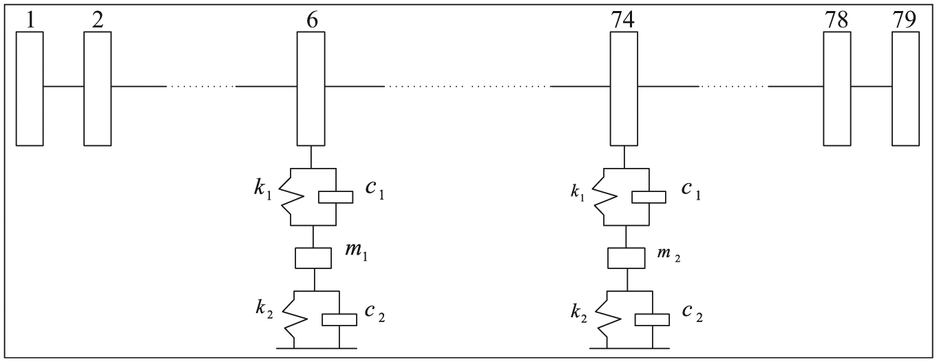
The discretization model of rotor.

Nodes 6 and 74 are the locations of the metal rubber bearing of the magnetic bearing. $k_{1}$ is the support stiffness of bearing and $k_{2}$ is the support stiffness of metal rubber ring. $c_{1}$ is the support stiffness of bearing and $c_{2}$ is the support stiffness of metal rubber ring. $m_{1}$ and $m_{2}$ are the mass of two radial magnetic bearings.

Finite element modeling of flexible rotor is a common tool for rotor dynamics analysis. The magnetic rotor bearing is an elastic system with continuous mass distribution. It can simplify the rotor to a multi-degree-of-freedom system with limited lumped mass. The basic idea of the finite element method is to divide the whole rotor into a finite element according to the node. Each element is connected to each other at a node, so that the motion of a rotor with continuous mass distribution is dispersed into the motion with finite degrees of freedom. The more the element number of the rotor, the more accurate the model is, but the amount of calculation is greatly increased.

The two adjacent nodes of the flexible rotor are used as the basic element of the finite element analysis, which is called the elastic shaft segment element, as shown in Figure 3. The left end is the i node and the right end is the $i + 1$ node. The space coordinates of each shaft segment can be expressed by the displacement vectors of the two ends, known as the generalized coordinates of the shaft segment. The displacement vector of the ends can be expressed by the axis coordinates x and y and deflection angles $θ_{y}$ and $θ_{x}$ as

\begin{matrix} U_{i} = {[\begin{matrix} x_{i} & y_{i} & θ_{i, y} & θ_{i, x} \end{matrix}]}_{i}^{T} \\ U_{i + 1} = {[\begin{matrix} x_{i + 1} & y_{i + 1} & θ_{i + 1, y} & θ_{i + 1, x} \end{matrix}]}_{i}^{T} \end{matrix}

(1)

Figure 3.

The elastic shaft segment element.

According to the lumped parameter method, starting from the rotor node 1, the four state vectors at the right end are calculated according to the boundary constraints of the left end, and then, the state parameters at the right end of the adjacent segment are calculated.

Hence, we establish the dynamic equation of each shaft segment element. Without considering the effects of shear and torsional deformation, the dynamic differential equations of an elastic shaft segment element in the two directions of x and y are

\begin{matrix} [m_{x}] {{\overset{\cdot\cdot}{u}}_{x}} + [d_{x}] {{\overset{\cdot}{u}}_{x}} - ω [g_{x}] {{\overset{\cdot}{u}}_{y}} + [k_{x}] {u_{x}} = {f_{x}} \\ [m_{y}] {{\overset{\cdot\cdot}{u}}_{y}} + [d_{y}] {{\overset{\cdot}{u}}_{y}} - ω [g_{y}] {{\overset{\cdot}{u}}_{x}} + [k_{y}] {u_{y}} = {f_{y}} \end{matrix}

(2)

where $ω$ is the angular velocity of rotor and ${f_{x}}$ and ${f_{y}}$ are the generalized external force vector on x and y directions at the element of the elastic axis, respectively. $[m_{x}]$ , $[d_{x}]$ , $[g_{x}]$ , and $[k_{x}]$ and $[m_{y}]$ , $[d_{y}]$ , $[g_{y}]$ , and $[k_{y}]$ are the mass matrix, damping matrix, gyro matrix, and stiffness matrix on the x and y directions at the element, respectively. They are all $4 \times 4$ matrix.

According to the finite element method, after listing the dynamic equations of each shaft segment based on the connection relationship between adjacent elements, each element equation can be integrated into a large matrix dynamic equation of the rotor as

[M] {\overset{\cdot\cdot}{U}} + ([D] + ω [G]) {\overset{\cdot}{U}} + [K] {U} = {F}

(3)

where ${F}$ is the generalized external force vector, $[M]$ is the mass matrix, $[K]$ is the stiffness matrix, $[D]$ is the damping matrix, and $[G]$ is the gyro matrix. Since the rotor of AMB is suspended without contact, the internal damping is 0, and the damping matrix $[D]$ is a zero matrix. The equivalent damping of AMB is reflected in the electromagnetic force by the form of external damping. The electromagnetic bearing support is the external force of the rotor at the position of the electromagnetic bearing node

In the small-square stand for the corresponding $[m]$ , $[g]$ , and $[k]$ matrix of each element, they are arranged diagonally and overlap the $2 \times 2$ parts of the adjacency matrix. The upper part of $[M]$ , $[K]$ , and $[G]$ is the dynamic equation of the x plane, and the inferior part is the dynamic equation of the y plane. They are all $4 N \times 4 N$ order sparse symmetric matrix.

At the non-supported and non-rotor ends, the dynamic equations are as follows

M_{i} {\overset{\cdot\cdot}{U}}_{i} + G_{i} {\overset{\cdot}{U}}_{i} + K_{i}^{1} U_{i - 1} + K_{i}^{2} U_{i} + K_{i}^{3} U_{i} + K_{i}^{4} U_{i + 1} = F_{i}

(7)

where $U_{i}$ is the state vector of node i, $M_{i}$ is the mass matrix of node i, $K_{i} = [\begin{matrix} K_{i}^{1} & K_{i}^{2} & K_{i}^{3} & K_{i}^{4} \end{matrix}]$ is the stiffness matrix of node $i - 1$ , i, and $i + 1$ , and $F_{i}$ is the generalized external force vector of node i.

Where

U_{i} = {[\begin{matrix} x_{i} & y_{i} & θ_{i, y} & θ_{i, x} \end{matrix}]}_{i}^{T}

M_{i} = {[\begin{matrix} m & 0 & 0 & 0 \\ 0 & m & 0 & 0 \\ 0 & 0 & J_{y} & 0 \\ 0 & 0 & 0 & J_{x} \end{matrix}]}_{i}^{T} G_{i} = {[\begin{matrix} 0 & 0 & 0 & 0 \\ 0 & 0 & 0 & 0 \\ 0 & 0 & 0 & - J_{z} ω \\ 0 & 0 & J_{z} ω & 0 \end{matrix}]}_{i}^{T}

\begin{matrix} K_{I}^{1} = {[\begin{matrix} - 12 EI / l^{3} & 0 & - 6 EI / l^{2} & 0 \\ 0 & - 12 EI / l^{3} & 0 & - 6 EI / l^{2} \\ 6 EI / l^{3} & 0 & 2 EI / l & 0 \\ 0 & 6 EI / l^{2} & 0 & 2 EI / l \end{matrix}]}_{i}^{T} \\ K_{I}^{2} = {[\begin{matrix} 12 EI / l^{3} & 0 & - 6 EI / l^{2} & 0 \\ 0 & 12 EI / l^{3} & 0 & - 6 EI / l^{2} \\ - 6 EI / l^{3} & 0 & 4 EI / l & 0 \\ 0 & - 6 EI / l^{2} & 0 & 4 EI / l \end{matrix}]}_{i}^{T} \\ K_{I}^{3} = {[\begin{matrix} 12 EI / l^{3} & 0 & 6 EI / l^{2} & 0 \\ 0 & 12 EI / l^{3} & 0 & 6 EI / l^{2} \\ 6 EI / l^{3} & 0 & 4 EI / l & 0 \\ 0 & 6 EI / l^{2} & 0 & 4 EI / l \end{matrix}]}_{i}^{T} \\ K_{I}^{4} = {[\begin{matrix} - 12 EI / l^{3} & 0 & 6 EI / l^{2} & 0 \\ 0 & - 12 EI / l^{3} & 0 & 6 EI / l^{2} \\ - 6 EI / l^{3} & 0 & 2 EI / l & 0 \\ 0 & - 6 EI / l^{2} & 0 & 2 EI / l \end{matrix}]}_{i}^{T} \end{matrix}

where $J_{x}$ and $J_{y}$ stand for the moment of inertia of the diameter of the x axis and the y axis, respectively; $J_{z}$ stands for the polar moment of inertia of the z axis. I is the section inertia moment of shaft segment, and $I = π d^{4} / 64$ , where d is the diameter of the shaft segment, l is the length of the shaft segment, and E is the elastic modulus of the material.

The two ends of the rotor are in free state and are not affected by external force and torque. Thus, the dynamic equation of element 1 is as follows

M_{1} {\overset{\cdot\cdot}{U}}_{1} + G_{1} {\overset{\cdot}{U}}_{1} + K_{1}^{3} U_{1} + K_{1}^{4} U_{2} = F_{1}

(8)

The dynamic equation of element 79 is as follows

M_{79} {\overset{\cdot\cdot}{U}}_{79} + G_{79} {\overset{\cdot}{U}}_{79} + K_{79}^{1} U_{79} + K_{1}^{2} U_{79} = F_{79}

(9)

We choose element 1 to analyze the influence of the rotational speed parameters on the chaotic behavior of the system.

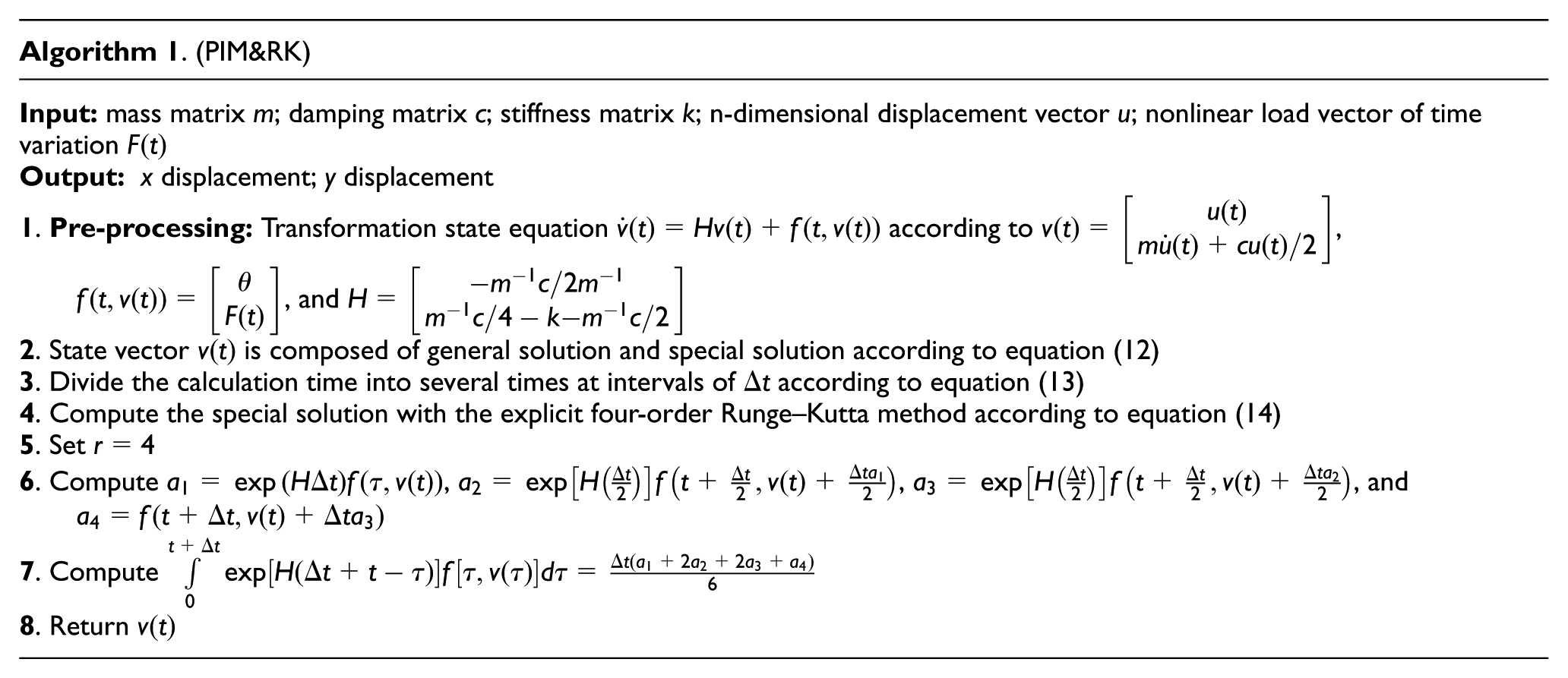
The PIM&RK method

In this section, the PIM&RK method is introduced. The dynamic equation with finite element discretization can be written as follows

m \overset{\cdot\cdot}{u} (t) + c \overset{\cdot}{u} (t) + ku (t) = F (t)

(10)

where m is the mass matrix, c is the damping matrix, k is the stiffness matrix, n is the degree of freedom of the structure system, and u is the n-dimensional displacement vector. $F (t)$ is the nonlinear load vector of time variation.

Transform equation (10) into a first-order state equation¹⁹ as follows

\overset{\cdot}{v} (t) = Hv (t) + f (t, v (t))

(11)

where

\begin{matrix} v (t) = [\begin{matrix} u (t) \\ m \overset{\cdot}{u} (t) + cu (t) / 2 \end{matrix}] \\ f (t, v (t)) = [\begin{matrix} θ \\ F (t) \end{matrix}] \\ H = [\begin{matrix} - m^{- 1} c / 2 & m^{- 1} \\ m^{- 1} c / 4 - k & - m^{- 1} c / 2 \end{matrix}] \end{matrix}

where $v (t)$ is the 2n dimensional state vector, $f (t, v (t))$ is the 2n dimensional force correlation vector, and H is the 2n × 2n dimensional constant matrix.

Equation (11) is composed of two parts: general solution and special solution as

v (t) = \exp (Ht) v (0) + \int_{0}^{t} \exp [H \cdot (t - τ)] f [τ, v (τ)] d τ

(12)

The first item in the right-hand is a general solution, and the second item of the right end is a special solution. The calculation time is divided into several time intervals of $Δ t$ .The response relation between $t + Δ t$ and t time system response can be obtained from equation (12) as

v (t + Δ t) = \exp (H Δ t) v (t) + \int_{0}^{t + Δ t} \exp [H (Δ t + t - τ)] f [τ, v (τ)] d τ

(13)

The second term on the right side of equation (13) is Duhamel. It is obtained by the fourth-order RK method as

\int_{0}^{t + Δ t} \exp [H (Δ t + t - τ)] f [τ, v (τ)] d τ = Δ t \sum_{i = 1}^{r} ρ_{i} a_{i}

(14)

where $a_{1} = \exp (H Δ t) f (τ, v (t))$ and

a_{k} = \exp [H Δ t (1 - h_{k})] f (t + h_{k} Δ t, v (t) + Δ t \sum_{j = 1}^{k - 1} (γ_{k j} a_{j})), k = 2, \dots, r

where r is the order of RK and $ρ_{i}$ , $h_{k}$ , and $γ_{kj}$ are the control parameters.

Let $r = 4$ , obtaining an integral expression with fourth-order accuracy

\int_{0}^{t + Δ t} \exp [H (Δ t + t - τ)] f [τ, v (τ)] d τ = \frac{Δ t (a_{1} + 2 a_{2} + 2 a_{3} + a_{4})}{6}

(15)

where

\begin{matrix} a_{2} = \exp [H (\frac{Δ t}{2})] f (t + \frac{Δ t}{2}, v (t) + \frac{Δ t a_{1}}{2}) \\ a_{3} = \exp [H (\frac{Δ t}{2})] f (t + \frac{Δ t}{2}, v (t) + \frac{Δ t a_{2}}{2}) \\ a_{4} = f (t + Δ t, v (t) + Δ t a_{3}) \end{matrix}

Calculating $a_{1}$ based on $v (t)$ , forward $Δ t$ and forecast system state $v (t) + a_{1} Δ t / 2$ by $a_{1}$ , and calculate $a_{2}$ and then reforecast system state $v (t) + a_{2} Δ t / 2$ by $a_{2}$ and calculate $a_{3}$ . Reforecast system state $v (t) + a_{3} Δ t / 2$ by $a_{3}$ and calculate $a_{4}$ . The final calculation is obtained through the prediction from $a_{1}$ to $a_{4}$ .

Thus, the predictive correction calculation from $a_{1}$ to $a_{4}$ instead of the iterative operation is required for the implicit integration method. The PIM&RK method is formed by Algorithm 1.

Algorithm 1. (PIM&RK)
Input: mass matrix m; damping matrix c; stiffness matrix k; n-dimensional displacement vector u; nonlinear load vector of time variation $F (t)$
Output: x displacement; y displacement
1. Pre-processing: Transformation state equation $\overset{\cdot}{v} (t) = Hv (t) + f (t, v (t))$ according to $v (t) = [\begin{matrix} u (t) \\ m \overset{\cdot}{u} (t) + cu (t) / 2 \end{matrix}]$ , $f (t, v (t)) = [\begin{matrix} θ \\ F (t) \end{matrix}]$ , and $H = [\begin{matrix} - m^{- 1} c / 2 & m^{- 1} \\ m^{- 1} c / 4 - k & - m^{- 1} c / 2 \end{matrix}]$
2. State vector $v (t)$ is composed of general solution and special solution according to equation (12)
3. Divide the calculation time into several times at intervals of $Δ t$ according to equation (13)
4. Compute the special solution with the explicit four-order Runge–Kutta method according to equation (14)
5. Set $r = 4$
6. Compute $a_{1} = \exp (H Δ t) f (τ, v (t))$ , $a_{2} = \exp [H (\frac{Δ t}{2})] f (t + \frac{Δ t}{2}, v (t) + \frac{Δ t a_{1}}{2})$ , $a_{3} = \exp [H (\frac{Δ t}{2})] f (t + \frac{Δ t}{2}, v (t) + \frac{Δ t a_{2}}{2})$ , and $a_{4} = f (t + Δ t, v (t) + Δ t a_{3})$
7. Compute $\int_{0}^{t + Δ t} \exp [H (Δ t + t - τ)] f [τ, v (τ)] d τ = \frac{Δ t (a_{1} + 2 a_{2} + 2 a_{3} + a_{4})}{6}$
8. Return $v (t)$

Lyapunov exponent analysis

Lyapunov exponent depicts the discrete extent between two adjacent trajectories in the phase plane, which clearly divides the deterministic motion and the chaotic motion.

For continuous systems, there are

X = G (X (τ), τ) X \in R^{n} τ \in R

(16)

Let $\bar{X} (τ)$ be a datum trajectory and $X (τ)$ be its adjacent trajectory. We define the norm of $X = [\begin{matrix} x_{1} & x_{2} & \dots & x_{n} \end{matrix}]^{T}$ as follows

‖ X ‖ = \sqrt{\sum_{i = 1}^{n} x_{i}^{2}}

(17)

The discrete extent of the distance between $X (τ)$ and $\bar{X} (τ)$ with time is as follows

δ X (τ) =^{del} X (τ) - \bar{X} (τ)

(18)

Let $‖ δ X (τ_{0}) ‖$ be sufficiently small at time $τ_{0}$ , and then, the one-dimensional Lyapunov exponent is defined as follows

λ = lim_{τ \to \infty} \frac{1}{τ - τ_{0}} \ln \frac{‖ δ X (τ) ‖}{‖ δ X (τ_{0}) ‖}

(19)

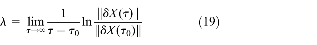
In the n-dimensional continuous system, $δ X (τ)$ has components on each substrate. Each component can be calculated by equation (19) for a $λ$ . Thus, existing n Lyapunov exponents, called Lyapunov exponent spectra. If the largest Lyapunov exponent $λ_{max} > 0$ , the system must be in chaos. Thus, we can calculate the largest Lyapunov exponent to identify whether the system is in chaos.

For the system, the effect of speed on chaos is shown in Figure 4.

Figure 4.

Lyapunov exponent of rotor system.

Figure 4 presents the largest Lyapunov exponent $λ_{max} > 0$ when the speed is 4800–5000 and 10,000–12,000 r/min. For this rotor, the first- and second-order critical speeds are found near 5294 and 10,900 r/min, respectively, and the system should be in chaos. Arredondo et al.⁵ proposed flexible rotor with modal shapes at different speeds, and the chaos appeared are also different. It will be verified in the simulation.

Simulation

In this section, we use the sliding mode controller¹⁰ to show the numerical calculation results produced by RK and PIM&RK methods. The AMB system is a complex system with multiple inputs, multiple outputs, strong nonlinearity, and high coupling degree. The reliability and stability depend largely on the control method of the system. The conventional PID control theory cannot be used very well. Although the combination of PID and other control strategies is highly accurate, the control system design is complex. The sliding mode controller is insensitive to internal parameters and external disturbances and has good robustness, which can effectively improve running performance of the system.²⁰ We compare their accuracy with our proposed method to prove its validity and do the chaos analysis based on the results.

Simulation setting

In this section, the parameters of the current AMB system are shown in Table 1.

Table 1.

AMB system parameters.

Parameters	Symbol	Value	Unit
Mass	M	7.5322	kg
Diameter moment of inertia	$J_{x}$	0.4624	kg m²
Diameter moment of inertia	$J_{y}$	0.4624	kg m²
Polar moment of inertia	$J_{z}$	0.0032	kg m²
Elastic modulus of material	E	$186 \times 10^{9}$	N/m²
Total length of rotor	l	828	mm
Diameter of rotor	d	40	mm

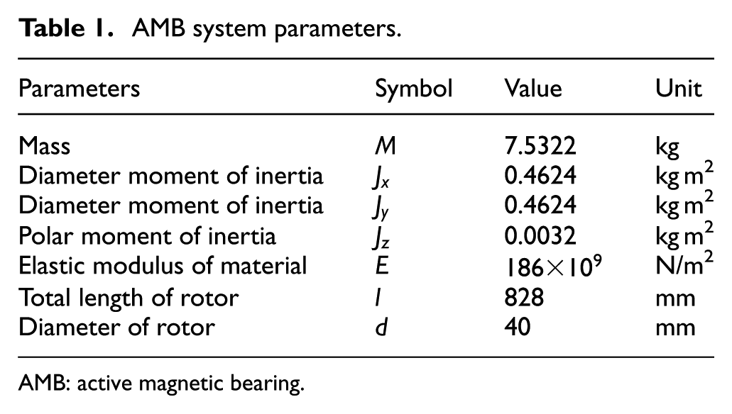
AMB: active magnetic bearing.

Simulation procedure

As to equation (8), we use the PIM&RK method to resolve the dynamic equations with differential rotor speeds around first and second critical speeds under the control of sliding mode controller. Then, we make trajectory, y direction displacement images, and chaos analysis based on the calculation results. Next, we make a comparison with RK. Finally, we evaluate and calculate performance of PIM&RK based on the results of three different steps.

Simulation results and analysis

In section 3, we have theoretically made a chaotic analysis of the rotor at two critical speeds through largest Lyapunov exponents. In this section, we detect the first- and second-order critical speed to verify the results obtained. The trajectory and y direction displacement of the rotor at element 1 and chaos analysis with different speeds are shown. In addition, the effectiveness of our proposed method is evaluated by experimenting different steps and comparing with RK method.

Chaos analysis

Figure 5 illustrates the trajectory and y direction displacement of the rotor at element 1 at the speed of 4800 r/min. The rotor does not get into chaos at this speed and is in a steady state of periodic motion.

Figure 5.

Trajectory and y direction displacement of the rotor at element 1 $(ω = 4800 r / \min)$ : (a) controlled trajectory and (b) y direction displacement.

Figure 6 illustrates the trajectory and y direction displacement of the rotor at element 1 at a speed of 5000 r/min. At this speed, the rotor just arrived in the chaos state and entered the critical state of the quasi-periodic motion.

Figure 6.

Trajectory and y direction displacement of the rotor at element 1 $(ω = 5000 r / min)$ : (a) controlled trajectory and(b) y direction displacement.

Figure 7 illustrates the trajectory and y direction displacement of the rotor at element 1 at a speed of 5500 r/min. At this speed, the rotor reaches the second-order critical speed of the rotor, entering chaos, and there is a divergent trend in the trajectory of the rotor at this time.

Figure 7.

Trajectory and y direction displacement of the rotor at element 1 $(ω = 5500 r / min)$ : (a) controlled trajectory and(b) y direction displacement.

From Figures 5 –7, when the speed is close to the critical speed, the rotor trajectory gradually comes into an extremely complex unstable state of motion from the periodic motion.

Figure 8 illustrates the trajectory and y direction displacement of the rotor at element 1 at speed for 8000 r/min. Under the control of the sliding mode controller, the rotor does not get into chaos at this speed and is in a steady state of periodic motion.

Figure 8.

Trajectory and y direction displacement of the rotor at element 1 $(ω = 8000 r / min)$ : (a) controlled trajectory and(b) y direction displacement.

Figure 9 illustrates the trajectory and y direction displacement of the rotor at element 1 at speed for 10,000 r/min. At this speed, the rotor begins to approach the second-order critical speed, and the rotor just arrived in the chaos state and entered the critical state of the quasi-periodic motion, similar to the state of 5000 r/min.

Figure 9.

Trajectory and y direction displacement of the rotor at element 1 $(ω = 10, 000 r / min)$ : (a) controlled trajectory and(b) y direction displacement.

Figure 10 illustrates the trajectory and y direction displacement of the rotor at element 1 at the speed of 11,000 r/min. At this speed, the rotor reaches the second-order critical speed, and there is a divergent trend in the trajectory of the rotor at this time, and the system displacement is in the unstable state of chaotic motion.

Figure 10.

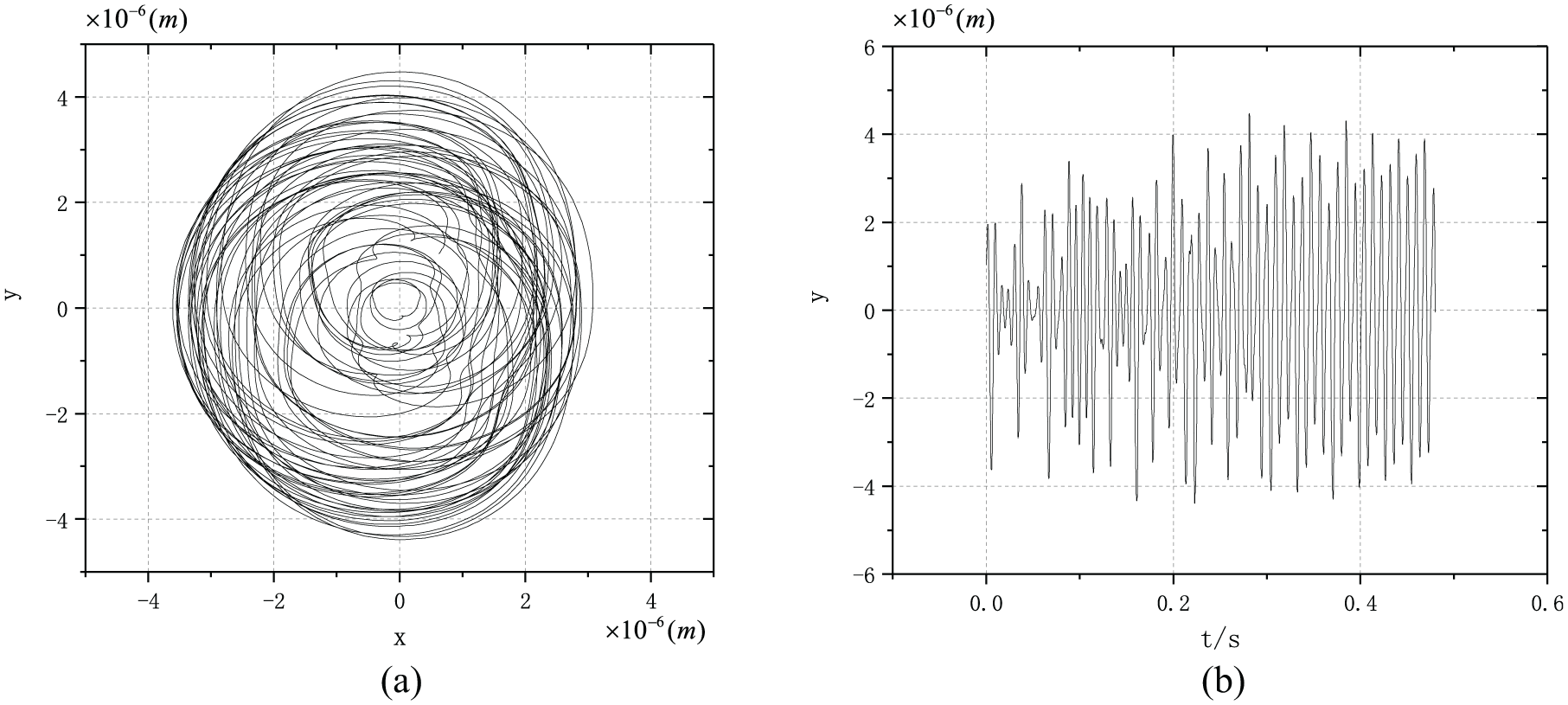
Trajectory and y direction displacement of the rotor at element 1 $(ω = 11, 000 r / \min)$ : (a) controlled trajectory and(b) y direction displacement.

From Figure 10, we can see that compared with the first critical speed, chaos is more serious with different mode shapes at the second-order critical speed. Figure 11 illustrates the rotor movement process at element 1 for 0.32 s at the speed of 11,000 r/min, and it also presents the process of how the rotor begins its quasi-periodic motion into chaos. From Figures 5 to 11, we can see that before entering the critical speed, the rotor trajectory can be in a regular and stable state, and with the increase in speed, the trajectory has a divergent trend; continuing at this speed, the rotor from the stable state to an unstable state that confined to a certain area and the trajectory is extremely complicated.

Figure 11.

Rotor movement process at element 1 for 0.32 s $(ω = 11, 000 r / min)$ .

Performance comparison with previous approaches

We check the accuracy of RK and PIM&RK for chaotic analysis with the speed of 11,000 r/min. The correctness and accuracy of the results of the PIM&RK method are evaluated by numerical experiments using comparison test of x displacement with RK method in 0.05 s at 11,000 r/min. The results are shown in Figure 12.

Figure 12.

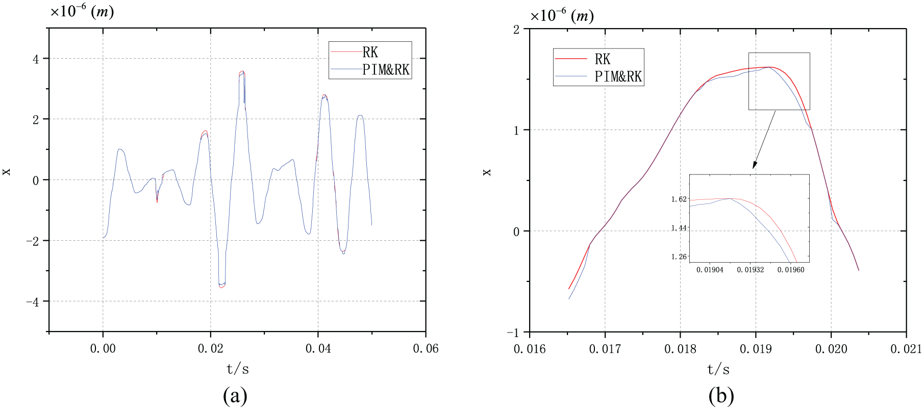
x direction displacement with $Δ t = 1 \times 10^{- 4} s$ .

Figure 12 presents the result of the RK method and the PIM&RK method with the integral step $Δ t = 1 \times 10^{- 4} s$ , and the simulation result of two methods tallies. Further increasing the integral step $Δ t$ , it is found that the convergent result cannot be obtained by the RK method.

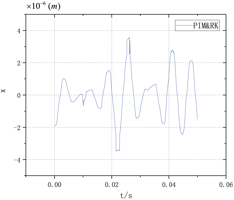
In Figure 13, the convergent result of the PIM&RK method is given under the condition of $Δ t = 4 \times 10^{- 4} s$ , which is four times the increase in the integral step. A good convergence result is obtained.

Figure 13.

x direction displacement with the integral step $Δ t = 4 \times 10^{- 4} s$ .

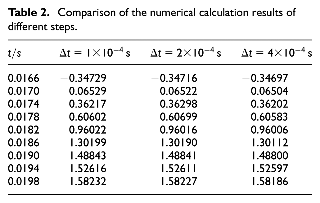
The numerical calculation results of the PIM&RK method are reported in Table 1 for $Δ t = 1 \times 10^{- 4} s$ , $Δ t = 2 \times 10^{- 4} s$ , and $Δ t = 4 \times 10^{- 4} s$ . From Table 2, we can see that the PIM&RK methods maintain high accuracy in different steps for $Δ t = 1 \times 10^{- 4} s$ , $Δ t = 2 \times 10^{- 4} s$ , and $Δ t = 4 \times 10^{- 4} s$ , and the calculation results are basically the same (see also Zhang et al.¹¹). The accuracy is not reduced with the increase in step. And the results are shown in Figure 14.

Table 2.

Comparison of the numerical calculation results of different steps.

$t / s$	$Δ t = 1 \times 10^{- 4} s$	$Δ t = 2 \times 10^{- 4} s$	$Δ t = 4 \times 10^{- 4} s$
0.0166	−0.34729	−0.34716	−0.34697
0.0170	0.06529	0.06522	0.06504
0.0174	0.36217	0.36298	0.36202
0.0178	0.60602	0.60699	0.60583
0.0182	0.96022	0.96016	0.96006
0.0186	1.30199	1.30190	1.30112
0.0190	1.48843	1.48841	1.48800
0.0194	1.52616	1.52611	1.52597
0.0198	1.58232	1.58227	1.58186

Figure 14.

PIM&RK with different integral step.

In Figure 14(a), the x displacement in 0.016–0.019 s is presented, and in Figure 14(b), the x displacement in 0.0164–0.0172 s is presented. From Figure 14(a) and (b), we can see that x displacements coincide at the same time t. Consistent with the results in Table 2, the smaller the step size, the more accurate the x-vibration image obtained. Thus, the high accuracy is verified according to the results of Table 2 and Figure 14. PIM&RK still maintain high accuracy, which increases the integral step. We can increase the integral step to simplify the calculation while calculating more simulation data points.

Conclusion

Concerning the finite element model of the AMB system obtained by unitization, the rotor is divided into 79 nodes. And the model is simplified to describe the dynamic characteristics of the flexible rotor.

A novel method for dynamic equation calculation—the precise Runge-Kutta hybrid integration method as well as the process of using the largest Lyapunov exponent to identify chaos with speed change is introduced.

The conventional RK method and the PIM&RK method are used to perform the dynamic equations solution and numerical simulation for the flexible rotor of AMB system. The results show that the calculation effects of the PIM&RK method are better than those of the RK method. When the integral step is four times increased, PIM&RK maintains high accuracy, and the convergent result cannot be obtained by RK. And the analysis result shows that compared with the first critical speed, chaos is more serious with different mode shapes at the second-order critical speed. It is helpful to design the controller to cross the critical speed smoothly and protect the rotor.

Footnotes

Handling Editor: Francesco Massi

Declaration of conflicting interests

The author(s) declared no potential conflicts of interest with respect to the research, authorship, and/or publication of this article.

Funding

The author(s) disclosed receipt of the following financial support for the research, authorship, and/or publication of this article: This work was supported by the National Natural Science Foundation of China (grant nos 61573012 and 61702388) and Fundamental Research Funds for Central University (WUT: 2016A004).

ORCID iD

Dongbo Zhang

References

Jiang

WH.

Singularity analysis of Jeffcott rotor-magnetic bearing with time delays. Appl Math 2012; 27: 419–427.

Sun

Bai

et al . Analysis and design of permanent magnet biased magnetic bearing based on hybrid factor. Adv Mech Eng 2016; 8: 33623.

Wan

Yang

Sun

et al . Decoupling control of a 5-degree-of-freedom bearingless induction motor based on least squares support vector machine inverse. Adv Mech Eng 2016; 8: 72120.

Sun

Zhao

et al . Identification of active magnetic bearing system with a flexible rotor. Mech Syst Signal Pr 2014; 49: 302–316.

Arredondo

Jugo

Etxebarria

Modeling and control of a flexible rotor system with AMB-based sustentation. ISA T 2008; 47: 101–112.

Evdokimov

Izosimova

Davydov

AV.

Automatic control system of active magnetic suspension in turbomachine rotor. Russ Aeronaut 2015; 57: 307–314.

Mao

Han

Liu

et al . Bearing dynamic parameters identification of a flexible rotor-bearing system based on transfer matrix method. Inverse Probl Sci En 2016; 24: 372–392.

Arias-Montiel

Silva-Navarro

. Finite element modeling and unbalance compensation for a two disks asymmetrical rotor system. In: Proceedings of the 5th international conference on electrical engineering, computing science and automatic control, Mexico, 12–14 May 2008, pp.386–391. New York: IEEE.

Han

Zhang

Dynamics balancing technology based on flexible rotor analysis. Tool Eng 2016; 50: 86–90.

10.

Jang

Chen

Tsao

YM.

Sliding mode control for active magnetic bearing system with flexible rotor. J Franklin Inst 2005; 342: 401–419.

11.

Zhang

Deng

A precise Runge-Kutta integration and its application for solving nonlinear dynamical systems. Appl Math Comput 2007; 184: 496–502.

12.

Xia

Zhang

et al . Non-iterative solving algorithm for coupled vibration of a train-bridge system based on precise Runge-Kutta hybrid integration method. J Vib Shock 2013; 32: 39–969.

13.

Tombul

Banks

SP.

Nonlinear optimal control of rotating flexible shaft in active magnetic bearings. Sci China Technol Sci 2011; 54: 1084–1094.

14.

Cha

Kuznetsov

Glavatskih

A comparative linear and nonlinear dynamic analysis of compliant cylindrical journal bearings. Mech Mach Theory 2013; 64: 80–92.

15.

Sadri

CQ.

Modified Lyapunov exponent, new measure of dynamics. Nonlinear Dynam 2014; 78: 2731–2750.

16.

Tung

Tsai

Chen

et al . Design of model-based unbalance compensator with fuzzy gain tuning mechanism for an active magnetic bearing system. Expert Syst Appl 2011; 38: 12861–12868.

17.

Chen

Tung

Tsai

et al . A self-tuning fuzzy PID-type controller design for unbalance compensation in an active magnetic bearing. Expert Syst Appl 2009; 36: 8560–8570.

18.

Ding

Zhou

ZD.

Effects of magnetic pole arrangement on magnetic field and force in radial magnetic bearings. China Mech Eng 2008; 19: 2364–2367.

19.

Zhang

Deng

WP.

Simplified computation of precise immediate integration method for structure dynamic equation. J Dynam Control 2008; 6: 107–112.

20.

Huynh

Tran

MHQ

. Integral sliding mode control approach for 3-pole active magnetic bearing system. Appl Mech Mater 2016; 829: 128–132.

Chaos of flexible rotor system with critical speed in magnetic bearing based on the improved precise Runge–Kutta hybrid integration

Abstract

Keywords

Introduction

Related work

Finite element modeling of magnetic bearing with flexible rotor system

The PIM&RK method

Lyapunov exponent analysis

Simulation

Simulation setting

Simulation procedure

Simulation results and analysis

Chaos analysis

Performance comparison with previous approaches

Conclusion

Footnotes

Declaration of conflicting interests

Funding

ORCID iD

References