Wavelet multi-resolution approximation of time-varying frame structure

Abstract

Engineering structures usually exhibit time-varying behavior when subjected to strong excitation or due to material deterioration. This behavior is one of the key properties affecting the structural performance. Hence, reasonable description and timely tracking of time-varying characteristics of engineering structures are necessary for their safety assessment and life-cycle management. Due to its powerful ability of approximating functions in the time–frequency domain, wavelet multi-resolution approximation has been widely applied in the field of parameter estimation. Considering that the damage levels of beams and columns are usually different, identification of time-varying structural parameters of frame structure under seismic excitation using wavelet multi-resolution approximation is studied in this article. A time-varying dynamical model including both the translational and rotational degrees of freedom is established so as to estimate the stiffness coefficients of beams and columns separately. By decomposing each time-varying structural parameter using one wavelet multi-resolution approximation, the time-varying parametric identification problem is transformed into a time-invariant non-parametric one. In solving the high number of regressors in the non-parametric regression program, the modified orthogonal forward regression algorithm is proposed for significant term selection and parameter estimation. This work is demonstrated through numerical examples which consider both gradual variation and abrupt changes in the structural parameters.

Introduction

Structural health monitoring (SHM) is to characterize the potential damage and further to predict the remaining service life for engineering structures using advanced sensing technology and data mining techniques. ¹ In the last three decades, SHM has received great attention in multidisciplinary fields spanning a wider spectrum of engineering areas including aerospace, civil, mechanical, electrical, and electronic engineering.^2–6 As one of the key components in SHM, structural system identification (SSI) is to extract structural information from observed dynamical responses in conjunction with a proper structural modeling technique and parameter estimation method.^7–9 In the area of SSI, most methods developed assume that the structural systems are time invariant and correspondingly their structural parameters are constant within the observed time period. However, under the action of natural disasters such as strong wind or seismic excitation, engineering structures usually exhibit time-varying behavior due to damage accumulation and aging. ¹⁰ This behavior is actually one of the key properties affecting the structural performance. Hence, reasonable description and timely tracking of time-varying characteristics for engineering structures are necessary for their safety assessment and life-cycle management.

A certain number of methods have been proposed to tackle the time-varying parameter estimation problem in SSI. The frequently used approaches are those based on the piecewise constant theory^11,12 and those using online/recursive estimation with forgetting factors.^13–16 Recently, adoption of time–frequency analysis tools such as Hilbert–Huang transform (HHT)^17–19 or wavelet transform (WT)^20–27 has been taken for time-varying identification. Since fewer assumptions on the dynamical modeling or the behavior of time-varying parameters are made, it is more versatile to track both the slowly or fast varying behavior in the parameters. As one of the time–frequency analysis tools, WT is powerful and efficient for the characterization of time-varying features and the parsimonious representation of non-stationary signals. ²⁸ An early study in Tsatsanis and Giannakis ²⁰ was to represent the time-varying parameters using separate sets of wavelet filter banks. The time-varying problem was then transformed to select the significant regressors in a regression modeling problem. This approach makes the wavelet multi-resolution approach a promising tool for time-varying system identification. In Ghanem and Romeo, ²¹ a wavelet-based time-varying system identification procedure for the parameters characterizing discrete mechanical systems was presented. The approach projected the governing differential equation onto a subspace constructed from wavelets and time-varying parameters were estimated from the input and output noisy data. In Basu, ²² a WT approach was proposed to identify the variation of stiffness in structural systems, where both sudden and gradual changes for single-degree-of-freedom (SDOF) and multiple-degree-of-freedom (MDOF) systems were considered. Xu et al. ²³ developed a wavelet-based state space method to identify both modal parameters and structural parameters using both free vibration and forced vibration data.

In previous works,^24–27 different applications of wavelet multi-resolution approximation (WMRA) to time-varying structural identifications have been made. For those methods using WMRA to quantify time-varying structural properties, however, only shear-type structures were considered as the applications, and consequently the time-varying behaviors of individual components cannot be assessed. Practically, the structures are usually more complicated than the idealized shear-type ones, and structural damage often starts at a local structural component and develops progressively at different components with time. Therefore, it is necessary to develop techniques which can not only properly track the time-varying behavior but also locate the components with the time-varying behavior. In this work, a model-based time-varying parameter identification technique is developed to track both time-varying stiffness and damping coefficients of frame structures using WMRA. A time-varying dynamical model including both translational and rotational degrees of freedom (DOFs) is established. Thus, the different contribution to the dynamic structural responses from the beams and columns can be identified separately. By decomposing each time-varying structural parameter using one WMRA, the problem of time-varying parametric estimation is converted to a time-invariant non-parametric case. In solving the high number of regressors in the non-parametric regression problem, the modified orthogonal forward regression (OFR) algorithm is proposed for the purpose of a robust estimation by selecting significant terms.

In the following sections, the theory of WMRA is first presented. Then, the modeling of the time-varying dynamical system and the identification procedure are given. Finally, illustrative examples considering both gradual and abrupt changes in time-varying parameters are presented.

WMRA

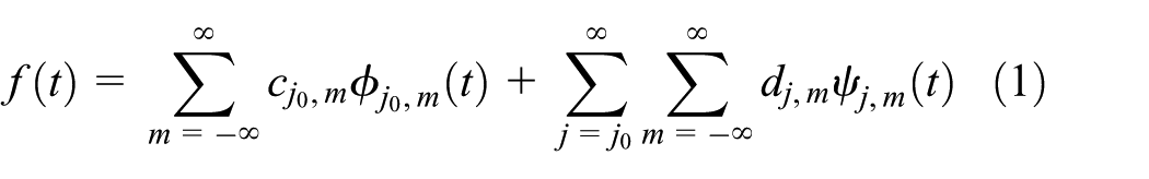
As a result of a multidisciplinary effort from mathematicians, physicists, and engineers, wavelet theory has been applied in plenty of areas, especially in areas of signal processing, non-parametric estimation, and data compression. ²⁸ With its good localization properties in both time and frequency, wavelet analysis is powerful in characterizing non-stationary functions/signals. WMRA is one of the most popular applications of wavelet theory in signal processing by representing a signal into coarse and detail components at different scale levels. For any finite energy function/signal in continuous time, its WMRA can be expressed as ²⁸

$$f(t)=\sum _{m=-\infty }^{\infty }{c}_{j_0,m}{\varphi }_{j_0,m}(t)+\sum _{j=j_0}^{\infty }\sum _{m=-\infty }^{\infty }{d}_{j,m}{\psi }_{j,m}(t)$$

(1)

where the basis functions $\{{\varphi }_{j_0,m}(t),{\psi }_{j,m}(t)\}$ are ${\varphi }_{j_0,m}(t)=2^{j_0/2}\varphi (2^{j_0}t-m)$ with scale level $j_0$ and translation $2^{-j_0}m$ of the scaling function $\varphi (t)$ , and ${\psi }_{j,m}(t)=2^{j/2}\psi (2^{j}t-m)$ with scale level j and translation $2^{-j}m$ of the mother wavelet function $\psi (t)$ , respectively, and $c_{j_0,m}$ and $d_{j,m}$ are the corresponding expansion coefficients. The first summation on the right-hand side of equation (1) is the coarse component of $f(t)$ at the initial scale level $j_0$ and the other summation is the detail component of $f(t)$ , in which the detail at the higher scale level $j$ gives the finer information. Typically, the finite energy signal can be accurately represented by a truncated version of WMRA up to the scale level J since the details at higher scale levels than J have little contribution to the signal. The scale level J which represents the WMRA resolution level usually depends on the frequency bandwidth of the signal.

The truncated version of WMRA for the discrete signal $f[k],k=0,1,\dots ,N_t-1$ with length $N_t$ can be derived as ²⁶

$$f\left[k\right]\approx a+\sum _{j=0}^{J-1}\sum _{m=m_0}^{m_j}{d}_{j,m}\psi (2^{j-j_0}k-m)$$

(2)

where for a best coarse approximation of the discrete signal the initial scale level is determined by $j_0=\mathrm{int}({\log }_2{N}_t)$ with $\mathrm{int}(·)$ being the round-up integer function, and the summation bounds for m depend on both the data length $N_t$ and the support width of the mother wavelet. Taking the type of Daubechies wavelet (dbN) for example, the values for the summation bounds are $m_0=2-2N$ and $m_j=\mathrm{int}(2^{j-j_0}{N}_t)-1$ . ²⁶ In equation (2), the constant coarse a is applied since there exists an intercorrelation among the scaling functions and wavelet functions at the scale level $j=0$ . Furthermore, when $J=1$ is used in equation (2), it means that the signal is approximated by the constant a only.

For convenience in the derivations in the later section, a matrix representation of equation (2) is used

$$\mathbf{f}\approx \mathbf{w}(J)\mathbf{\beta }(J)$$

(3)

where $\mathbf{f}=[\begin{array}{cccc}f[0]\hfill & f[1]\hfill & \cdots \hfill & f[N_t-1]\hfill \end{array}{]}^T$ , $\mathbf{\beta }=[a{d}_{0,m_0}\cdots d_{j,m}\cdots {]}^T$ , and $\mathbf{w}$ is the wavelet reconstruction matrix corresponding to each element of $\mathbf{\beta }$ . Note that the size of the reconstruction matrix and the number of expansion coefficients depend on the resolution level. It should be pointed out that depending on the chosen type of mother wavelet the WMRA of a signal is not unique and the corresponding approximation performance would also be different. As mentioned in Ahuja et al., ²⁹ the choice of wavelet type for a good representation is usually application dependent. With its orthogonal and compact support properties, the dbN wavelet has been used in many applications for system identification.^27,30,31 Therefore, the Daubechies wavelet is again adopted in this work.

Parametric identification of time-varying frame structure using WMRA

Since the damage levels in the beams and the columns of the frame structure under operation are usually different, it is therefore necessary to develop an identification technology which can estimate the properties of the beams and columns separately. In the following, the proposed time-varying parametric identification of the beam and column members of the frame structure using WMRA is described.

Dynamical model of time-varying frame structure

A time-varying dynamical model including both translational and rotational DOFs is established so that the different contributions to the dynamic responses from the beams and columns can be separated and therefore it is possible to estimate their individual properties. The equations of motion for an N-story linear time-varying frame building under seismic excitation can be written as

$$\mathbf{M}\stackrel{\mathbf{··}}{\mathbf{u}}(t)+\mathbf{C}(t)\stackrel{.}{\mathbf{u}}(t)+\mathbf{K}(t)\mathbf{u}(t)=\mathbf{\gamma }{\stackrel{··}{\mathbf{x}}}_g(t)$$

(4)

where the mass matrix $\mathbf{M}$ can be usually considered as time invariant, the time-varying damping matrix $\mathbf{C}(t)$ models the damping behavior, the time-varying stiffness matrix $\mathbf{K}(t)$ contains information of both beams and columns, $\mathbf{u}(t)$ is the relative translational and rotational displacement vector with respect to the ground, $\stackrel{·}{\mathbf{u}}(t)$ and $\stackrel{··}{\mathbf{u}}(t)$ are the vectors of the velocity and acceleration, respectively, ${\stackrel{··}{\mathbf{x}}}_g(t)$ is the ground acceleration vector, and $\mathbf{\gamma }$ is the distribution matrix of the effective forces on the structure corresponding to the ground acceleration components. Without loss of generality, only plain frame structure under translational ground acceleration ${\stackrel{··}{x}}_g(t)$ is considered in the following context. The purpose of this study is to estimate the time-varying damping coefficients and the stiffness coefficients of both beams and columns using the measured structural responses and earthquake excitation.

Using the finite element method, the system matrices relating to the DOFs in equation (4) can be constructed. For example, the form of the element mass and stiffness matrices is given in equation (5) when axial deformation can be neglected ³²

$${\mathbf{M}}_e=\frac{\bar{m}L}{420}\left[\begin{array}{cccc}156& 54& 22L& -13L\\ 54& 156& 13L& -22L\\ 22L& 13L& 4L^2& -3L^2\\ -13L& -22L& -3L^2& 4L^2\end{array}\right],{\mathbf{K}}_e=\frac{2i_e(t)}{L^2}\left[\begin{array}{cccc}6& -6& 3L& 3L\\ -6& 6& -3L& -3L\\ 3L& -3L& 2L^2& L^2\\ 3L& -3L& L^2& 2L^2\end{array}\right]$$

(5)

where $\bar{m}$ denotes the uniform mass density of the element and L denotes the element length. The consistent mass form of each element is considered here but the lumped mass type is also suitable. For the element stiffness matrix, the linear stiffness $i_e(t)=\mathrm{EI}(t)/L$ is considered as a time-varying parameter reflecting the time-varying property of the member such as the beam or column, where $\mathrm{EI}(t)$ is the time-varying cross-sectional stiffness of the element.

Due to the difficulty and complexity of damping modeling, a simplified version of viscous damping without coupling between the velocities is used as

$$\mathbf{C}(t)=\mathrm{diag}\left[\begin{array}{cccccc}{c}_1(t)\hfill & c_2(t)\hfill & \cdots \hfill & c_n(t)\hfill & \cdots \hfill & c_{N_d}(t)\hfill \end{array}\right]$$

(6)

where $c_n(t)$ is the time-varying damping coefficient corresponding to the nth velocity DOF in equation (4), $N_d$ is the total number of DOFs considered for the frame structure, and $\mathrm{diag}[·]$ is an operator to covert the damping coefficient vector into a diagonal matrix.

Time-varying regression model formulation for the frame structure

Assuming that the mass matrix is measurable or known and all the dynamical response quantities, including the displacements, velocities, and accelerations, and the ground acceleration can be measured or calculated, the identification problem is to estimate the time-varying stiffness coefficients of beams and columns, and the damping coefficients for the frame structure. With all the known quantities, equation (4) can be revised by

$$\mathbf{\gamma }{\widehat{\stackrel{··}{x}}}_{\mathbf{g}}(t)\mathbf{-}\mathbf{M}\widehat{\stackrel{··}{\mathbf{u}}}(t)\mathbf{=}\mathbf{C}(t)\widehat{\stackrel{·}{\mathbf{u}}}(t)\mathbf{+}\mathbf{K}(t)\hat{\mathbf{u}}(t)\mathbf{+}\mathbf{\epsilon }(t)$$

(7)

where $\widehat{•}\mathrm{denotes}$ the corresponding measured quantity and $\mathbf{\epsilon }\mathbf{(}T\mathbf{)}$ is the error vector due to the measurement noise and modeling error.

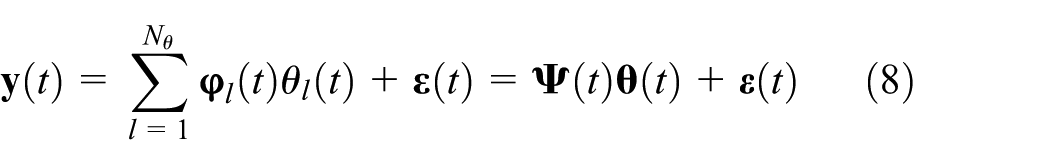
Then, equation (7) can be written into a time-varying regression model for identification as

$$\mathbf{y}(t)=\sum _{l=1}^{N_{\theta }}{\mathbf{\phi }}_l(t){\theta }_l(t)+\mathbf{\epsilon }(t)\mathbf{=}\mathbf{\Psi }(t)\mathbf{\theta }(t)\mathbf{+}\mathbf{\epsilon }(t)$$

(8)

where $\mathbf{y}(t)=\mathbf{\gamma }{\widehat{\stackrel{··}{x}}}_g(t)-\mathbf{M}\widehat{\stackrel{··}{\mathbf{u}}}(t)$ is the regression output, $\mathbf{\theta }(t)=[\begin{array}{cccc}{\theta }_1(t)\hfill & {\theta }_2(t)\hfill & \cdots \hfill & {\theta }_{N_{\theta }}(t)\hfill \end{array}{]}^T$ represents the time-varying parameter including the stiffness information of all beams and columns, and the damping coefficients in equation (6), and $\mathbf{\Psi }(t)=[\begin{array}{cccc}{\mathbf{\phi }}_1(t)\hfill & {\mathbf{\phi }}_2(t)\hfill & \cdots \hfill & {\mathbf{\phi }}_{N_{\theta }}(t)\hfill \end{array}]$ is the matrix consisting of all regressors ${\mathbf{\phi }}_l(t)$ corresponding to each time-varying parameter ${\theta }_l(t)$ . Note that the regressors ${\mathbf{\phi }}_l(t)$ are constructed from the measured response quantities and the structural form of the stiffness and damping matrices in equation (7). Denote the discrete-time response data as $\mathbf{y}[k]=\mathbf{y}(t_k)$ , $t_k=k\Delta t$ , $k=0,1,...,N_t-1$ where $\Delta t$ is the sampling time step and $N_t$ is the finite length of data. Then, the matrix form of equation (8) for all time sequences can be expressed as

$$\mathbf{Y}=\mathbf{\Phi }\mathbf{\Theta }\mathbf{+}\mathbf{E}$$

(9)

where

$$\begin{array}{c}\mathbf{Y}={\left[\begin{array}{cccc}{\mathbf{y}}^T\left[0\right]\hfill & {\mathbf{y}}^T\left[1\right]\hfill & \cdots \hfill & {\mathbf{y}}^T[N_t-1]\hfill \end{array}\right]}^T\hfill \\ \mathbf{\Phi }=\mathbf{\left[}\begin{array}{cccc}\mathbf{\Psi }\mathbf{\left[}0\mathbf{\right]}\hfill & \mathbf{0}\hfill & \cdots \hfill & \mathbf{0}\hfill \\ \multicolumn{1}{c}{\mathbf{0}}& \mathbf{\Psi }\mathbf{\left[}\mathbf{1}\mathbf{\right]}\hfill & \cdots \hfill & \mathbf{0}\hfill \\ \multicolumn{1}{c}{⋮}& ⋮\hfill & \mathbf{\ddots }\hfill & ⋮\hfill \\ \multicolumn{1}{c}{\mathbf{0}}& \mathbf{0}\hfill & \cdots \hfill & \mathbf{\Psi }[N_t-1]\hfill \end{array}\mathbf{\right]}\hfill \\ \mathbf{\Theta }={\mathbf{\left[}\begin{array}{cccc}{\mathbf{\theta }}^T\mathbf{\left[}0\mathbf{\right]}\hfill & {\mathbf{\theta }}^T\mathbf{\left[}1\mathbf{\right]}\hfill & \cdots \hfill & {\mathbf{\theta }}^T\mathbf{[}{N}_t-1\mathbf{]}\hfill \end{array}\mathbf{\right]}}^T\hfill \\ \mathbf{E}={\mathbf{\left[}\begin{array}{cccc}{\mathbf{\epsilon }}^T\mathbf{\left[}0\mathbf{\right]}\hfill & {\mathbf{\epsilon }}^T\mathbf{\left[}1\mathbf{\right]}\hfill & \cdots \hfill & {\mathbf{\epsilon }}^T\mathbf{[}{N}_t-1\mathbf{]}\hfill \end{array}\mathbf{\right]}}^T\hfill \end{array}$$

As a time-varying regression problem, the solution for $\mathbf{\Theta }$ is usually non-unique theoretically due to the fact that the number of unknowns in $\mathbf{\Theta }$ is usually larger than the length of $\mathbf{Y}$ . Thus, it is preferable to develop feasible ways to properly track each time-varying parameter. In the following, an approach is proposed by expanding each time-varying parameter using WMRA. It is assumed that each time-varying parameter changes continuously and smoothly over time and only with a small number of sudden change locations so that each time-varying parameter can be effectively represented through only a small number of significant basis functions and the solution to the corresponding regression problem is unique.

Time-varying parameter identification using WMRA

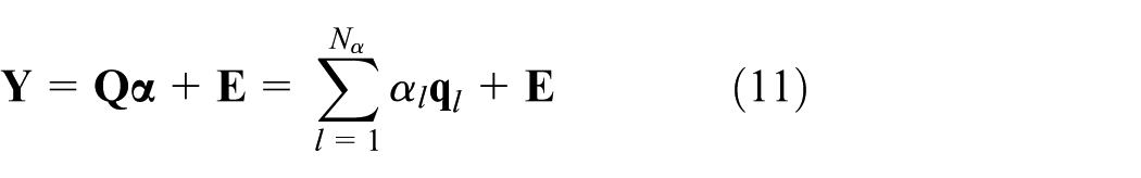
Using the WMRA model in equation (3) to represent each time-varying parameter, the parameter vector $\mathbf{\Theta }$ can be expressed in the matrix form as

$$\mathbf{\Theta }=\mathbf{W}\mathbf{\alpha }$$

(10)

where $\mathbf{\alpha }=\{\mathbf{a},{\mathbf{d}}_{j,m}\}\mathbf{\in }{\mathbb{R}}^{N_{\alpha }\times 1}$ is the vector of the WMRA expansion coefficients for all time-varying parameters and $\mathbf{W}$ is the corresponding WMRA reconstruction matrix. In $\mathbf{\alpha }$ , $\mathbf{a}\in {\mathbb{R}}^{N_{\theta }\times 1}$ is the vector of WMRA constant values for all time-varying parameters. It should be pointed out that since different WMRA models are used to represent the time-varying parameters separately, the resolution levels used for different time-varying parameters may be different. For example, the resolution level for time-varying stiffness coefficients $J_i$ and that for time-varying damping coefficients $J_c$ may be different during identification.

Substituting equation (10) into equation (9), a time-invariant regression model can be obtained as

$$\mathbf{Y}=\mathbf{Q}\mathbf{\alpha }+\mathbf{E}=\sum _{l=1}^{N_{\alpha }}{\alpha }_l{\mathbf{q}}_l+\mathbf{E}$$

(11)

where the regression matrix $\mathbf{Q}=\mathbf{\Phi }\mathbf{W}$ contains both the measured responses in $\mathbf{\Phi }$ and the values of WMRA basis functions with different scale levels and translations, ${\alpha }_l$ is the $l\mathrm{th}$ coefficient of $\mathbf{\alpha }$ , ${\mathbf{q}}_l$ is the regressor vector corresponding to ${\alpha }_l$ , and $N_{\alpha }$ is the total number of unknown coefficients in WMRA. Thus, by decomposing each time-varying structural parameter using WMRA, the problem of time-varying parametric estimation is converted to the time-invariant non-parametric case. Then, the time-invariant coefficients can be solved using traditional least squares methods and the time-varying parameters can be reconstructed using equation (10). Note that the determination of the resolution levels for the time-varying structural parameters is important for parsimonious representation and accurate estimation. As described in the following subsection, if the resolution level is chosen to be too high, the whole estimation does not only require more computational time but may also result in an overfitting issue which will amplify the influence of measurement noise.

Selection of significant terms by the modified OFR algorithm

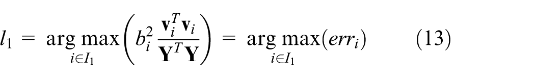
It should be pointed out that the number of unknown WMRA expansion coefficients $N_{\alpha }$ in equation (10) or (11) can be quite large even when using the truncated WMRA representation by equation (2). It thus makes the regression matrix generally singular when choosing high enough resolution levels to cover the time-varying trends in the time duration for identification. Therefore, applying the traditional least squares method to equation (11) directly to obtain the WMRA coefficients would lead to high fluctuations in the reconstructed time-varying parameters. Considering the fact that any finite energy function can be well approximated using only a few significant terms in WMRA due to the wavelets’ good local time–frequency properties, better estimation results are possible if those insignificant terms in equation (11) can be pruned beforehand when applying the least squares solution. The OFR algorithm ³³ which is an efficient significant term selection strategy is adopted here. The process of the OFR algorithm involves a stepwise Gram–Schmidt orthogonalization and sequentially reordering the regressor vectors ${\mathbf{q}}_l$ in $\mathbf{Q}$ according to their contribution to the regression output.

Note that the vector $\mathbf{a}$ in the WMRA coefficients can be considered as parameter values for the time-invariant case. Meanwhile, the coarse approximation by $\mathbf{a}$ usually includes more information to $\mathbf{Y}$ by WMRA. On the other hand, the time-varying trends in the structural parameters are captured by the wavelet expansion coefficients $\{{\mathbf{d}}_{j,m}\}$ . In order to avoid the unbalanced distribution among all parameters due to $\mathbf{a}$ and $\{{\mathbf{d}}_{j,m}\}$ , a modified OFR algorithm is proposed. It is performed in two OFR stages for the reordering of significant regressors corresponding $\mathbf{a}$ and $\{{\mathbf{d}}_{j,m}\}$ , respectively. The first stage is to consider all ${\mathbf{q}}_l$ corresponding to $\mathbf{a}$ (denoted as a-regressors hereafter) as significant terms and reorder them according to their significance. The second stage is to reorder the remaining ${\mathbf{q}}_l$ corresponding to $\{{\mathbf{d}}_{j,m}\}$ (denoted as d-regressors hereafter). By this, the new regressor matrix consisting of all significant terms is non-singular so that the reconstructed time-varying parameters can be more reliable. The detailed procedure of the proposed OFR is presented below.

It is assumed that all the regressors in equation (11) are pre-ordered with the first $N_{\theta }$ regressors corresponding to $\mathbf{a}$ . The first stage is to reorder the first $N_{\theta }$ a-regressors in $\mathbf{Q}$ .

Step $s=1$

Denote the set of locations a-regressors as $I_1=\{1,2,\dots ,N_{\theta }\}$ .

For all $i\in I_1$ , calculate

$${\mathbf{v}}_i={\mathbf{q}}_i,b_i=\frac{{\mathbf{v}}_i^T\mathbf{Y}}{{\mathbf{v}}_i^T{\mathbf{v}}_i}$$

(12)

$$l_1=\underset{i\in I_1}{\arg \max }(b_i^2\frac{{\mathbf{v}}_i^T{\mathbf{v}}_i}{{\mathbf{Y}}^T\mathbf{Y}})=\underset{i\in I_1}{\arg \max }({err}_i)$$

(13)

$${\mathbf{v}}_1^o={\mathbf{v}}_{l_1},{\mu }_1^o=b_{l_1},{ERR}_1=max({err}_i)={err}_{l_1}$$

(14)

Here, $l_1$ is the regressor location with the best error reduction ratio (ERR) score which contributes to $\mathbf{Y}$ among all the first $N_{\theta }$ regressors.

Step s, $1<s\le N_{\theta }$

Denote $I_s=I_{s-1}\backslash \{l_{s-1}\}$ , where \ indicates that the previous significant regressor location is removed.

For all $i\in I_s$ , calculate

$${\mathbf{v}}_i={\mathbf{q}}_i-\sum _{k=1}^{s-1}\frac{{{\mathbf{v}}_k^o}^T{\mathbf{q}}_i}{{{\mathbf{v}}_k^o}^T{\mathbf{v}}_k^o}{\mathbf{v}}_k^o,b_i=\frac{{\mathbf{v}}_i^T\mathbf{Y}}{{\mathbf{v}}_i^T{\mathbf{v}}_i}$$

(15)

$$l_s=\underset{i\in I_s}{\arg \max }(b_i^2\frac{{\mathbf{v}}_i^T{\mathbf{v}}_i}{{\mathbf{Y}}^T\mathbf{Y}})=\underset{i\in I_s}{\arg \max }({err}_i)$$

(16)

$${\mathbf{v}}_s^o={\mathbf{v}}_{l_s},{\mathbf{\mu }}_s^o=b_{l_s},{\mathbf{\lambda }}_{k,s}=-\frac{{{\mathbf{v}}_k^o}^T{\mathbf{q}}_{l_s}}{{{\mathbf{v}}_k^o}^T{\mathbf{v}}_k^o},{ERR}_s={err}_{l_s}$$

(17)

The above finishes the first stage of reordering the a-regressors. The following is the second stage of reordering the d-regressors using the previous orthogonalized regressors ${\mathbf{v}}_i$ .

Step s, $s>N_{\theta }$

Denote, for $s=N_{\theta }+1,I_s=\{N_{\theta }+1,N_{\theta }+2,\dots ,N_{\alpha }\}$ ; otherwise, $I_s=I_{s-1}\backslash \{l_{s-1}\}$ . The procedure to locate the significant terms is the same as in equations (15)–(17).

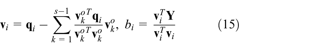
The purpose of performing the OFR algorithm is to simplify equation (11) by a sparse and accurate representation using only $N_s$ significant regressors as

$$\mathbf{Y}=\sum _{s=1}^{N_s}{\alpha }_{l_s}{\mathbf{q}}_{l_s}+\hat{\mathbf{E}}=\hat{\mathbf{Y}}+\hat{\mathbf{E}}$$

(18)

where ${\mathbf{q}}_{l_s}$ are all the significant regressors considered.

The OFR procedure continues until the following convergence criterion is met

$$ER=1-\frac{{\hat{\mathbf{Y}}}^T\hat{\mathbf{Y}}}{{\mathbf{Y}}^T\mathbf{Y}}=1-\sum _{s=1}^{N_s}{ERR}_s<{\rho }_e$$

(19)

where ER is defined as the error ratio (ER) between the fitted regression output $\hat{\mathbf{Y}}$ and the original regression output $\mathbf{Y}$ , and the tolerance value ${\rho }_e$ usually depends on the noise level. Theoretically, a smaller approximation error for $\mathbf{Y}$ can be achieved using a smaller ${\rho }_e$ . However, due to the existence of measurement noise in the measured data and modeling error, a too small ${\rho }_e$ can lead to an overfitting issue and also cause high irregularities in the reconstructed time-varying parameters. Since the noise level is usually unknown, the termination of OFR algorithm for significant term selection is conducted by choosing a proper error tolerance empirically based on the ER curve with respect to $N_s$ . As a sparse representation, usually $N_s$ is much smaller than the original number of regressors $N_{\alpha }$ .

The WMRA coefficients of the significant terms can be calculated backward from the values of ${\mu }_s^o$

$$\left[\begin{array}{c}{\alpha }_{l_1}\hfill \\ \multicolumn{1}{c}{{\alpha }_{l_2}}\\ \multicolumn{1}{c}{⋮}\\ \multicolumn{1}{c}{{\alpha }_{l_{N_s}}}\end{array}\right]=\left[\begin{array}{cccc}1\hfill & {\lambda }_{1,2}\hfill & \cdots \hfill & {\lambda }_{1,N_s}\hfill \\ \multicolumn{1}{c}{0}& 1\hfill & \cdots \hfill & {\lambda }_{2,N_s}\hfill \\ \multicolumn{1}{c}{⋮}& ⋮\hfill & \ddots \hfill & ⋮\hfill \\ \multicolumn{1}{c}{0}& 0\hfill & 0\hfill & 1\hfill \end{array}\right]\left[\begin{array}{c}{\mu }_1^o\hfill \\ \multicolumn{1}{c}{{\mu }_2^o}\\ \multicolumn{1}{c}{⋮}\\ \multicolumn{1}{c}{{\mu }_{N_s}^o}\end{array}\right]$$

(20)

where $l_s$ represents the position of the significant term and ${\alpha }_{l_s}$ is the corresponding WMRA expansion coefficient. Those expansion coefficients corresponding to the insignificant regressors in equation (11) are taken as zero. Finally, the time-varying parameters can be calculated using equation (10).

Illustrative examples

Practically speaking, frame structure is always in three-dimensional (3D) shape. However, for 3D frame structure without torsional effect under lateral loading, it can be separately analyzed for structural performance by a two-dimensional (2D) frame in each lateral direction. Hence, a one-bay two-story plain frame structure shown in Figure 1 was considered for the performance study of the proposed approach. The frame structure consists of six members including four story columns and two floor beams, and their corresponding linear stiffness coefficients were to be identified. As denoted in Figure 1, in order to model the dynamic behavior of the frame structure under seismic excitation, six DOFs are used where the four rotational DOFs are necessary to separate the stiffness contribution from the beams and columns. In addition, six damping coefficients corresponding to the six DOFs were also included during identification. Equation (21) gives the mass and stiffness matrices for the frame structure in Figure 1.

$$\begin{array}{c}\mathbf{M}=\frac{\bar{m}}{420}\left[\begin{array}{cccccc}624H+420L\hfill & 0\hfill & 0\hfill & 108H\hfill & 13H^2\hfill & 13H^2\hfill \\ \multicolumn{1}{c}{0}& 8H^3+4L^3\hfill & -3L^3\hfill & -13H^2\hfill & -3H^3\hfill & 0\hfill \\ \multicolumn{1}{c}{0}& -3L^3\hfill & 8H^3+4L^3\hfill & -13H^2\hfill & 0\hfill & -3H^3\hfill \\ \multicolumn{1}{c}{108H}& -13H^2\hfill & -13H^2\hfill & 312H+420L\hfill & 22H^2\hfill & 22H^2\hfill \\ \multicolumn{1}{c}{13H^2}& -3H^3\hfill & 0\hfill & 22H^2\hfill & 4H^3+4L^3\hfill & -3L^3\hfill \\ \multicolumn{1}{c}{13H^2}& 0\hfill & -3H^3\hfill & 22H^2\hfill & -3L^3\hfill & 4H^3+4L^3\hfill \end{array}\right]\hfill \\ \mathbf{K}=\left[\begin{array}{cccccc}\frac{12}{H^2}(i_{1l}+i_{1r}+i_{2l}+i_{2r})\hfill & \frac{6}{H}(i_{1l}-i_{2l})\hfill & \frac{6}{H}(i_{1r}-i_{2r})\hfill & -\frac{12}{H}(i_{2l}+i_{2r})\hfill & -\frac{6}{H}·i_{2l}\hfill & -\frac{6}{H}·i_{2r}\hfill \\ \multicolumn{1}{c}{\frac{6}{H}(i_{1l}-i_{2l})}& 4(i_{1l}+i_{1b}+i_{2l})\hfill & 2·i_{1b}\hfill & \frac{6}{H}·i_{2l}\hfill & 2·i_{2l}\hfill & 0\hfill \\ \multicolumn{1}{c}{\frac{6}{H}(i_{1r}-i_{2r})}& 2·i_{1b}\hfill & 4(i_{1r}+i_{1b}+i_{2r})\hfill & \frac{6}{H}·i_{2r}\hfill & 0\hfill & 2·i_{2r}\hfill \\ \multicolumn{1}{c}{-\frac{12}{H^2}(i_{2l}+i_{2r})}& \frac{6}{H}·i_{2l}\hfill & \frac{6}{H}·i_{2r}\hfill & \frac{12}{H^2}(i_{2l}+i_{2r})\hfill & \frac{6}{H}·i_{2l}\hfill & \frac{6}{H}·i_{2r}\hfill \\ \multicolumn{1}{c}{-\frac{6}{H}·i_{2l}}& 2·i_{2l}\hfill & 0\hfill & \frac{6}{H}·i_{2l}\hfill & 4(i_{2b}+i_{2l})\hfill & 2·i_{2b}\hfill \\ \multicolumn{1}{c}{-\frac{6}{H}·i_{2r}}& 0\hfill & 2·i_{2r}\hfill & \frac{6}{H}·i_{2r}\hfill & 2·i_{2b}\hfill & 4(i_{2b}+i_{2r})\hfill \end{array}\right]\hfill \end{array}$$

(21)

where the first index for the linear stiffness $i_{n·}$ indicates the story number and the second index indicates the left column $(l)$ , right column $(r)$ , or the beam $(b)$ , respectively. From the form of the stiffness matrix in equation (21), how each structural member contributes to the whole stiffness matrix is clearly reflected. For illustrative purpose, the same uniform mass density for all columns and beams was taken with $\bar{m}=240\mathrm{kg}/\mathrm{m}$ . The dimensions of the frame structure were $L=6\mathrm{m}\mathrm{and}H=5\mathrm{m}$ . The nominal (undamaged) values of the stiffness coefficients (N·m) were $i_{1l}=i_{1r}=i_{2l}=i_{2r}=4.0\times {10}^6$ for all column members and $i_{1b}=i_{2b}=3.5\times {10}^6$ for all beam members. As for the damping coefficients (N·s/m), the nominal values were $c_{1t}=5.0\times {10}^3$ , $c_{1l}=c_{1r}=1.0\times {10}^4$ , $c_{2t}=2.0\times {10}^3$ , and $c_{2l}=c_{2r}=7.0\times {10}^3$ for the translational and rotational DOFs at the 1st and 2nd floors, respectively. As a result, the six nominal natural frequencies of the structure are 16.1, 53.5, 119.4, 190.8, 239.6 and, 429 Hz, and the corresponding damping ratios are 1.54%, 2.08%, 2.31%, 2.73%, 3.09%, and 3.53%, respectively. The distribution vector of the effective forces on the six DOFs under translational ground acceleration is

$$\begin{array}{c}\multicolumn{1}{c}{\mathbf{\gamma }=-\frac{\bar{\mathbf{m}}}{420}[732\mathbf{H}\mathbf{+}420l-13{\mathbf{H}}^2-13{\mathbf{H}}^2}\\ \multicolumn{1}{c}{420(\mathbf{H}\mathbf{+}l)35{\mathbf{H}}^{2}35{\mathbf{H}}^2{]}^T}\end{array}$$

(22)

Figure 1.

One-bay two-story frame structure; $u_{n1}$ denotes the translational DOF of the nth floor, $u_{n2}$ denotes the left rotational DOF of the nth floor, and $u_{n3}$ denotes the right rotational DOF of the nth floor.

Considering that the properties of the frame structure may change gradually with time due to material deterioration and aging, or they may change abruptly from sudden damage under strong excitation, identification of the time-varying behaviors of the frame structure under these two working conditions is presented in the following.

Gradually varying case

In this case, linear reductions of the six stiffness coefficients were considered with $i_{1l}$ being reduced from 12th second to 20th second by 35%, $i_{1r}$ being reduced from the 11th second to the 20th second by 25%, $i_{1b}$ being reduced from the 6th second to the 18th second by 35%, $i_{2l}$ being reduced from the 8th second to the 18th second by 30%, $i_{2r}$ being reduced from the 9th second to the 18th second by 25%, and $i_{2b}$ being reduced from the 7th second to the 20th second by 30%. Meanwhile, linear increases of the six damping coefficients were $c_{1t}$ increased from the 8th second to the 19th second by 25%, $c_{1l}$ increased from the 9th second to the 19th second by 35%, $c_{1r}$ increased from the 7th second to the 19th second by 30%, $c_{2t}$ increased from the 6th second to the 15th second by 20%, $c_{2l}$ increased from the 7th second to the 17th second by 30%, and $c_{2r}$ increased from the 8th second to the 20th second by 25%.

Stationary random ground motion

The stationary random ground motion data shown in Figure 2 were first simulated as the seismic excitation to the frame structure. By this, the time-varying behaviors in the structural parameters are less affected by the source of non-stationary response amplitudes during identification. The response quantities including all the displacements, velocities, and accelerations were measured at a sampling frequency of 1 kHz for the duration of 25 s. Thus, the data length for identification is $N_t=25,001$ data and the initial WMRA scale for all structural parameters is $j_0=\mathrm{int}({\log }_2(N_t))=15$ .

Figure 2.

The stationary random ground motion and the structural dynamical responses of the 1st and 2nd floors.

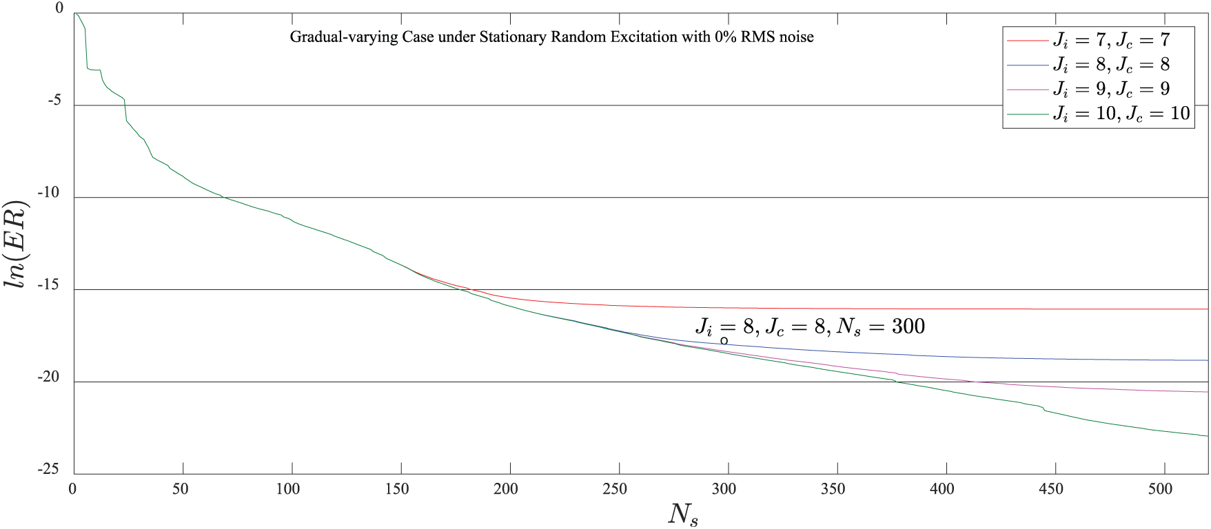
First, it was ideally assumed that there is no measurement noise on all responses. With the required response quantities available, the WMRA technique for estimating the time-varying stiffness and damping coefficients was applied. As aforementioned, a proper type of wavelet is necessary for applying the WMRA technique. Here, the db3 wavelet was chosen for the gradually varying case according to previous experiences.^9,30 As for the resolution levels for the time-varying parameters, they were determined by comparing the ER curves of several sets of resolution levels for stiffness and damping coefficients as shown in Figure 3. For each ER curve, the modified OFR scheme was applied to choose the significant terms for a robust estimation. From Figure 3, it can be seen that the regression output can be approximated quite well when using all the considered sets of resolution levels by noting the ER values $\ln (ER)<-15$ for $N_s>160$ . Note the fact that the higher the resolution level used, the better the fitting of the regression output. However, higher resolution level also needs higher computational effort while the tracking performance of the time-varying parameters will not be improved as long as the ER value reaches a certain value. Thus, it was decided to use the resolution levels with $J_i=J_c=8$ for this case. As a result, there were originally a total of 2580 WMRA coefficients before the OFR process and only a very small number of terms contributed significantly to the regression output after the OFR process. On the other hand, because there are no modeling error and measurement noise in this case, although the error ratio does not further reduce significantly with additional terms, the reconstructed time-varying parameters will be more accurate with a relatively larger number of significant terms. By balancing the computational effort and identification accuracy, finally $N_s=300$ was chosen to reconstruct the time-varying parameters. The reconstructed time-varying parameters are shown in Figure 4, indicating that all the time-varying parameters including both stiffness and damping coefficients were identified accurately. It should be pointed out that the results of damping concentrated on the translational DOFs are better than those concentrated on the rotational DOFs. This is because the response magnitudes corresponding to the translational DOFs are higher than those corresponding to the rotational DOFs by one order as shown in Figure 2.

Figure 3.

The ER curves for the selection of resolution levels and significant terms for the gradually varying case under stationary random ground motion (0% RMS noise).

Figure 4.

The identified time-varying stiffness (N·m) and damping (N·s/m) coefficients for the gradually varying case under stationary random ground motion (0% RMS noise).

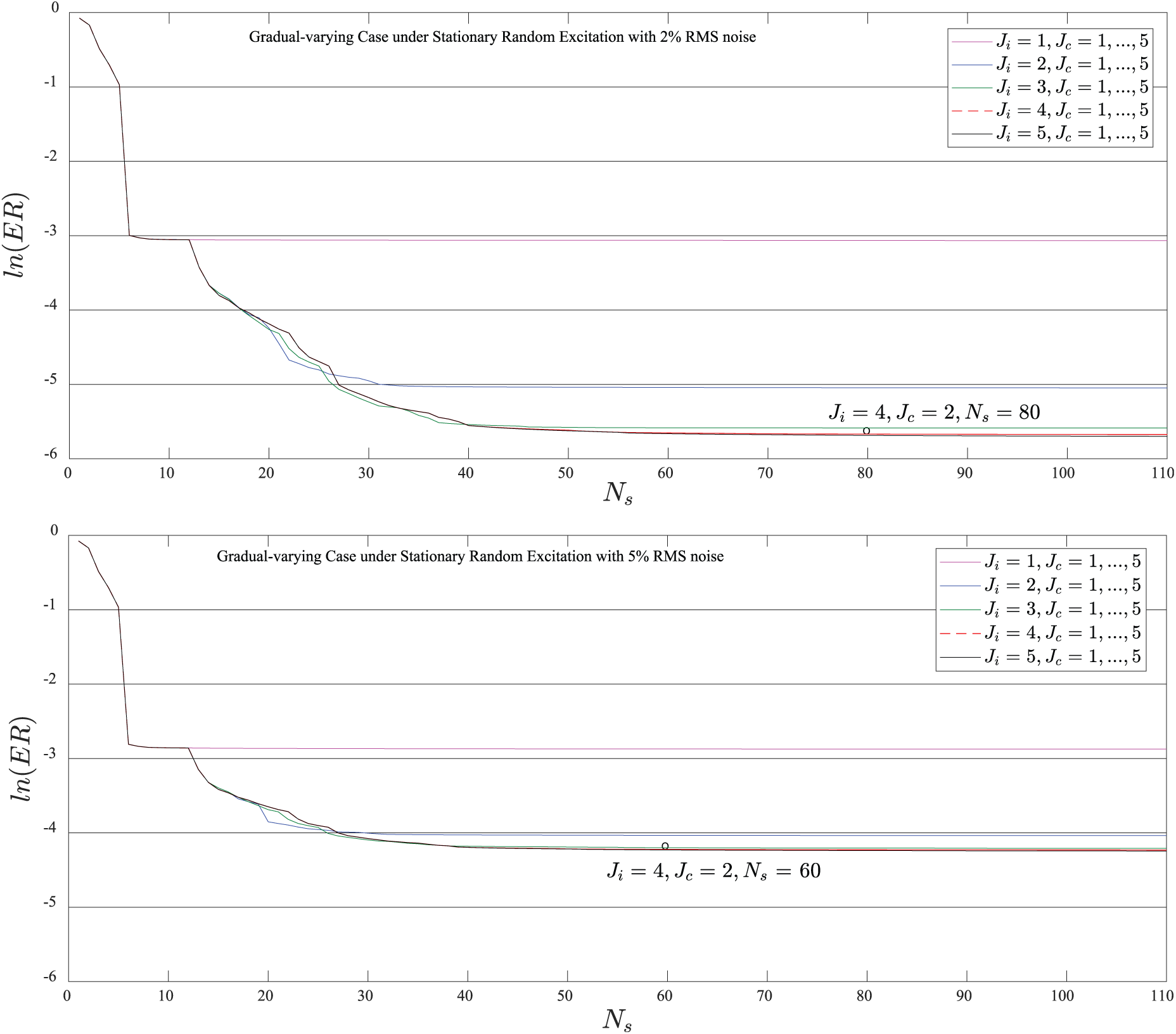
In practice, however, the measured responses are usually contaminated by noise. To study the effect of the measurement noise on the identification performance, independent Gaussian white noises with different levels of root mean square (RMS) were superimposed to all response quantities. It was found that directly applying the noisy measurements in the regressors can have a great influence on the identification results. Therefore, wavelet denoising ² of the measured responses with a soft threshold technique was performed before applying the WMRA approximation. Figure 5 shows the ER curves for different sets of resolution levels for the 2% and 5% RMS noise cases, respectively. It was found that the resolution levels for the damping coefficients made no difference on the ER curve due to their higher uncertainty in the presence of measurement noise than that of the stiffness coefficients. However, the increase of resolution levels for the stiffness coefficients affects the data fitting performance. The resolution levels with $J_i=4$ and $J_c=2$ were finally used according to the ER fitting performance. As a result, there were a total of 258 WMRA expansion coefficients. The final numbers of significant terms to reconstruct the time-varying parameters under 2% and 5% RMS were chosen to be only $N_s=80$ and $N_s=60$ , respectively. Compared with the 0% noise case, the number of significant terms is reduced significantly for the noisy cases. This indicates that the measurement noise can affect the estimation greatly in terms of the number of significant terms. The results also indicate that the higher the noise level, the less the number of significant terms. Figure 6 shows the reconstructed time-varying parameters using the selected number of significant terms, where the time-varying behavior of all the stiffness coefficients can be very accurately portrayed, while the time-varying damping coefficients are tracked only roughly. This result is expected because the contribution to the regression output from the regressors relating the damping coefficients is usually very small, resulting in a very few terms used to track the damping coefficients.

Figure 5.

The ER curves for the selection of resolution levels and significant terms for the gradually varying case under stationary random ground motion (2% and 5% RMS noise).

Figure 6.

The identified time-varying stiffness (N·m) and damping (N·s/m) coefficients for the gradually varying case under stationary random excitation (2% and 5% RMS noise).

Historical earthquake ground motion

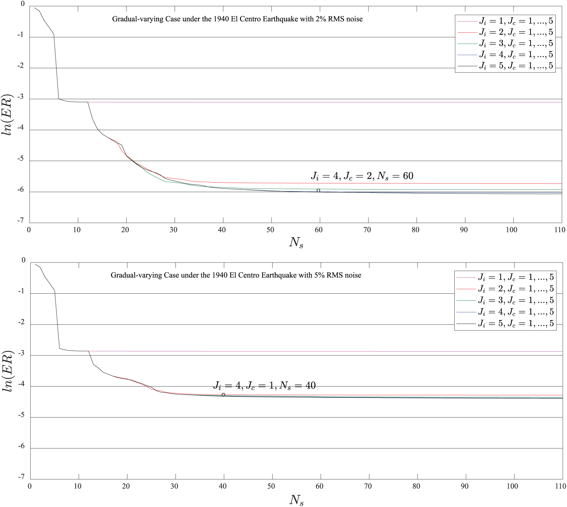
Previously, the proposed method was validated by stationary random excitation. Here, one historical earthquake record that is the North-South (NS) component of the ground acceleration of the 1940 El Centro earthquake was used to excite the structure to study the identification performance when the responses are non-stationary. The ground acceleration record and the dynamical responses are shown in Figure 7. Since the response amplitudes during the first 2 s were very small, the responses in this period were removed during identification. Thus, the data length for identification is $N_t=23,000$ data and correspondingly the initial scale is $j_0=15$ . The identification results of the case without noise contamination are similar to the case under stationary random ground motion and are not presented. Here only the identification results under noisy conditions are given. According to the ER curves in Figure 8, the resolution levels and the numbers of significant terms were chosen as $J_i=4,J_c=2,N_s=60$ and $J_i=4,J_c=1,N_s=40$ for the 2% and 5% RMS noise cases, respectively. Figure 9 shows the identified time-varying parameters which indicate that the accuracy of the stiffness coefficients is much better than that of the damping coefficients. As compared to the results under stationary random ground motion shown in Figure 6, the accuracy of the stiffness coefficients is slightly poor due to the non-stationarity of the responses. Again, due to much higher uncertainties in the estimated damping coefficients, only very rough trends or constant behaviors can be obtained.

Figure 7.

The NS component of the 1940 El Centro earthquake ground acceleration and the dynamical responses of the 1st and 2nd floors.

Figure 8.

The ER curves for the selection of resolution levels and significant terms for the gradually varying case under the 1940 El Centro earthquake (2% and 5% RMS noise).

Figure 9.

The identified time-varying stiffness (N·m) and damping (N·s/m) coefficients for the gradually varying case under the 1940 El Centro earthquake (2% and 5% RMS noise).

Effect of the randomness of noise

Furthermore, to account for the effect of the randomness of noise on the identification performance, 1000 independent sets of noises on the responses were simulated for statistical analysis. As observed previously that only very rough trends or constant values are obtained for the damping coefficients, in order to avoid the unnecessary influences on the statistical analysis from inconsistent locations of the significant terms for the damping coefficients, the damping coefficients were considered as time invariant during simulation and thus $J_c=1$ was used in WMRA approximation. However, the time-varying behaviors for the stiffness coefficients were still taken the same as those in the previous example with $J_i=4$ .

To quantity the estimation accuracy, an estimation error is defined as

$$e_{i_e}=\frac{1}{T}\underset{t_0}{\overset{t_0+T}{\int }}\frac{i_e(t)-{\hat{i}}_e(t)}{i_e(t)}\mathrm{dt}$$

(23)

where $t_0$ and T are the start time and the duration of data for identification and $i_e(t)$ and ${\hat{i}}_e(t)$ are the exact value and the identified stiffness value of the eth element, respectively. The estimation errors of the time-varying damping coefficients can be defined similarly. The statistics of estimation errors for both stiffness and damping coefficients are summarized in Tables 1 and 2 for the stationary random ground motion and the El Centro earthquake, respectively. In both tables, since there is no noise for the 0% RMS case, the estimation errors are obtained using one dynamic simulation. It can be seen that the estimations of both the stiffness and damping coefficients are nearly exact although the estimation errors of the damping coefficients are slightly higher for the 0% RMS case. On the other hand, by observing the standard deviations (SDs) of the stiffness parameters for both excitation cases with noise, it is shown that the levels of accuracy in the identification results are quite robust. The accuracy levels of the stiffness coefficients are over 99% and 97% for the 2% and 5% RMS cases, respectively, from the mean values. Regarding the damping coefficients, it can be observed that their estimation precisions are more uncertain than those of the stiffness coefficients by looking at both the mean values and SDs. This indicates that the damping coefficients are more difficult to be estimated. However, the accuracy levels of the damping coefficients higher than 90% are still quite reasonable.

Table 1.

The statistics of the estimation errors (%) for the gradually varying cases under stationary random ground motion.

Stiffness	0% RMS	2% RMS		5% RMS		Damping	0% RMS	2% RMS		5% RMS
	Mean	Mean	SD	Mean	SD		Mean	Mean	SD	Mean	SD
$i_{1l}$	0.004	0.485	0.072	1.366	0.077	$c_{1t}$	0.013	0.953	0.465	1.706	0.559
$i_{1r}$	0.003	0.432	0.072	1.343	0.036	$c_{1l}$	0.056	2.926	1.622	4.890	3.524
$i_{1b}$	0.003	0.505	0.092	1.626	0.024	$c_{1r}$	0.043	1.936	1.597	5.026	4.158
$i_{2l}$	0.004	0.708	0.143	2.406	0.063	$c_{2t}$	0.027	0.904	0.488	1.206	0.424
$i_{2r}$	0.003	0.666	0.144	2.370	0.134	$c_{2l}$	0.078	4.209	2.772	4.222	4.072
$i_{2b}$	0.004	0.715	0.140	2.488	0.141	$c_{2r}$	0.078	3.724	2.716	4.131	3.526

RMS: root mean square; SD: standard deviation.

Table 2.

The statistics of the estimation errors (%) for the gradually varying cases under the 1940 El Centro earthquake.

Stiffness	0% RMS	2% RMS		5% RMS		Damping	0% RMS	2% RMS		5% RMS
	Mean	Mean	SD	Mean	SD		Mean	Mean	SD	Mean	SD
$i_{1l}$	0.002	0.542	0.029	1.593	0.475	$c_{1t}$	0.026	0.752	0.053	3.577	0.476
$i_{1r}$	0.002	0.503	0.052	1.695	0.176	$c_{1l}$	0.085	5.310	0.075	5.110	0.415
$i_{1b}$	0.002	0.554	0.093	1.902	0.223	$c_{1r}$	0.050	1.200	0.237	4.697	1.861
$i_{2l}$	0.002	0.914	0.649	2.193	0.053	$c_{2t}$	0.010	0.732	0.039	3.239	0.192
$i_{2r}$	0.003	0.855	0.734	2.365	0.689	$c_{2l}$	0.092	5.234	1.156	8.397	4.127
$i_{2b}$	0.003	1.263	0.425	2.893	0.243	$c_{2r}$	0.067	3.713	0.598	5.127	0.980

RMS: root mean square; SD: standard deviation.

Figure 10 further illustrates the reconstructed time-varying parameters for the 1000 simulations with 2% RMS measurement noise under stationary random ground motion. It again shows that the stiffness coefficients are more accurate and robust than the damping coefficients.

Figure 10.

The identified time-varying stiffness (N·m) and damping (N·s/m) coefficients using 1000 sets of 2% RMS noise on responses for the gradually varying case under the stationary random ground motion.

Abruptly varying case

Abrupt changes in the structural parameters for identification were also considered. The reductions of the six stiffness coefficients considered were $i_{1l}$ reduced by 35% at the 12th second, $i_{1r}$ reduced by 25% at the 11th second, $i_{1b}$ reduced by 35% at the 6th second, $i_{2l}$ reduced by 30% at the 8th second, $i_{2r}$ reduced by 25% at the 9th second, and $i_{2b}$ reduced by 30% at the 7th second. Meanwhile, the increases of the six damping coefficients were $c_{1t}$ increased by 25% at the 8th second, $c_{1l}$ increased by 35% at the 9th second, $c_{1r}$ increased by 30% at the 7th second, $c_{2t}$ increased by 20% at the 6th second, $c_{2l}$ increased by 30% at the 7th second, and $c_{2r}$ increased by 25% at the 8th second. The identification procedure was the same as that in the gradually varying case with denoising of the noisy measurements beforehand. For the abrupt change case, the db1 wavelet was used because this type of wavelet is obviously the optimal for abruptly changing parameters. Only the identification results for the frame structure subjected to the 1940 El Centro excitation are presented here.

Figure 11 shows the ER behavior for the purpose of the determination of the resolution level and the number of significant terms under the 2% and 5% RMS noise cases, where the final resolutions and the numbers of significant terms are $J_i=8,J_c=1,N_s=60$ . In order to capture the abrupt changes in the structural parameters at different time instants, the resolution levels needed here are higher than those of the gradually varying case. Figure 12 shows the identified structural parameters, which indicates that all the time instants and extents of change in the stiffness coefficients are correctly identified. Although there exist small local fluctuations in the stiffness coefficients in Figure 12, the values return quickly to the actual values. Thus, it can be judged that small local fluctuations can be neglected during damage detection. As for the damping coefficients, similar to the gradually varying case, only very rough trends are obtained due to their high uncertainties in the presence of measurement noise. However, the level of accuracy in the estimation of the damping coefficients is still within the reasonable range.

Figure 11.

The ER curves for the selection of resolution levels and significant terms for the abruptly varying case under the 1940 El Centro earthquake (2% and 5% RMS noise).

Figure 12.

The identified time-varying stiffness (N·m) and damping (N·s/m) coefficients for the abruptly varying case under the 1940 El Centro earthquake (2% and 5% RMS noise).

Statistical analysis was also performed using simulations of 1000 sets of noises and the results are listed in Table 3. Similarly, it can be seen that the accuracy levels of the stiffness coefficients are over 99% and 97% for 2% and 5% RMS, respectively, from the mean values. On the other hand, it shows that the accuracy levels of the damping coefficients are rather uncertain by looking at both the mean values and SDs. This further indicates that the damping coefficients are more difficult to be tracked due to the high uncertainty in the presence of measurement noise. Only the coarse approximations of the damping coefficients can be tracked but the accuracy levels higher than 90% in the tables are still quite reasonable.

Table 3.

The statistics of the estimation errors (%) for the abruptly varying cases under the 1940 El Centro earthquake.

Stiffness	2% RMS		5% RMS		Damping	2% RMS		5% RMS
	Mean	SD	Mean	SD		Mean	SD	Mean	SD
$i_{1l}$	0.728	0.074	1.508	0.080	$c_{1t}$	4.866	0.252	4.685	0.382
$i_{1r}$	0.580	0.087	1.819	0.210	$c_{1l}$	6.678	1.591	6.400	0.426
$i_{1b}$	0.688	0.070	2.159	0.369	$c_{1r}$	4.268	10.542	3.879	2.232
$i_{2l}$	0.591	0.193	3.086	1.018	$c_{2t}$	2.162	1.019	2.176	0.897
$i_{2r}$	0.559	0.265	2.446	0.148	$c_{2l}$	7.577	4.400	7.678	8.412
$i_{2b}$	0.756	0.376	2.902	0.116	$c_{2r}$	5.682	3.562	4.947	4.129

RMS: root mean square; SD: standard deviation.

Conclusion

In this article, tracking of time-varying stiffness and damping parameters of frame structures under seismic excitation using WMRA is proposed. Rather than on the ideal shear-type buildings which were often considered in the literature, this work focuses on the identification of properties of individual structural members with time-varying characteristics. In order to identify the individual behavior of each structural component, both the translational and rotational DOFs are necessary to model the dynamic behavior of the frame structure. After that, using the WMRA to represent all the time-varying parameters of the frame structure, the problem of the time-varying parameter estimation is converted to a time-invariant non-parametric case. As a non-parametric regression analysis problem, initially there are usually a huge number expansion terms in approximating the regression output. In order to obtain the accurate and robust estimation results, the modified OFR algorithm is proposed to select the significant terms to both accurately and parsimoniously represent the regression output. ER curves are used to properly choose the resolution levels for the time-varying structural parameters. Examples illustrate that the time-varying damage levels of the stiffness coefficients inside the beams and the columns can be accurately estimated using the proposed method. The results are also robust in the presence of measurement noise. The levels of the damping coefficients are still reasonably estimated although only very rough behaviors are observed. Actually, the damping parameters are usually more uncertain to quantify than the stiffness coefficients.