Sage Journals: Discover world-class research

Abstract

When a natural gas transmission and distribution station performs a planned or emergency venting operation, the jet noise produced by the natural gas venting pipe can have an intensity as high as 110 dB, thereby severely affecting the production and living environment. Jet noise produced by venting pipes is a type of aerodynamic noise. This study investigates the mechanism that produces the jet noise and the radiative characteristics of jet noise using a computational fluid dynamics method that combines large eddy simulation with the Ffowcs Williams–Hawkings acoustic analogy theory. The analysis results show that the sound pressure level of jet noise is relatively high, with a maximum level of 115 dB in the low-frequency range (0–1000 Hz), and the sound pressure level is approximately the average level in the frequency range of 1000–4000 Hz. In addition, the maximum and average sound pressure levels of the noise at the same monitoring point both slightly decrease, and the frequency of the occurrence of a maximum sound pressure level decreases as the Mach number at the outlet of the venting pipe increases. An increase in the flow rate can result in a shift from low-frequency to high-frequency noise. Subsequently, this study includes a design of an expansion-chamber muffler that reduces the jet noise produced by venting pipes and an analysis of its effectiveness in reducing noise. The results show that the expansion-chamber muffler designed in this study can effectively reduce jet noise by 10–40 dB and, thus, achieve effective noise prevention and control.

Keywords

Upright venting pipe jet noise large eddy simulation Ffowcs Williams–Hawkings acoustic theory muffler

Introduction

Currently, four major types of pollution in the world are noise pollution, air pollution, exhaust gas pollution, and water pollution.^1–3 Noise pollution, a type of physical pollution, directly impinges on the ears of humans and has an instant effect, but it does not have a residual effect and will also not gradually accumulate.⁴ People will feel uncomfortable and have problems in concentrating and thinking when the noise level reaches 50 dB. A noise level greater than 80 dB will cause harm to people’s health. Those exposed to high-intensity noise for long periods of time may sustain hearing impairment or even permanent hearing loss and develop certain diseases.⁵

The venting system is an important component of a natural gas gathering and transportation station. Measurements have revealed that jet noise produced during a direct natural gas venting process has a sound pressure level (SPL) as high as 110 dB, which considerably exceeds the relevant national standard.^6,7

Jet noise produced by venting pipes is a type of aerodynamic noise. The acoustic analogy theory established by Lighthill⁸ in 1952, which marked the birth of aeroacoustics, divides a flow field into near- and far-fields and, thus, substantially simplifies the physical model of aeroacoustics. In 1955, Curle⁹ expanded Lighthill’s theory to consider the effect of static solid boundaries using the Kirchhoff method. In 1969, based on Curle’s results, Ffowcs Williams and Hawkings¹⁰ took into consideration the effect of solid boundaries on the sound produced by a fluid in motion using a generalized function and proposed the Ffowcs Williams–Hawkings equation (FW–H equation).

However, while the Curle and FW–H equations consider the effect of boundaries, they are both only applicable to static transmission media. In 1974, Goldstein¹¹ studied the sound produced by a fluid in a moving medium using the Green’s function method and obtained the universally applicable Lighthill equation. These classical equations and the Navier–Stokes equations are the foundation of modern aeroacoustics.

Computational aeroacoustics (CAA) is the combination of aeroacoustics and computational fluid dynamics. The basic idea of CAA is to predict the flow field and sound field by solving the Navier–Stokes equations. Because sound waves have a relatively wide frequency range, it is necessary to simulate the actual conditions of the flow field as accurately as possible, which, at the current stage, can only be achieved using direct numerical simulation (DNS) and large eddy simulation (LES). Freund et al.¹² were the first researchers to use DNS to predict the acoustic emission from turbulent jets. Freund simulated a supersonic jet flow with a Reynolds number (Re) of 2000 and a Mach number (Ma) of 1.92. The SPL of the simulated jet flow was basically in agreement with the measurement. In 2001, Freund¹³ simulated a subsonic jet flow with an Re of 3600 and an Ma of 0.9, and the predicted flow field and sound field were in agreement with the experimental data obtained by Stromberg et al.¹⁴ in 1980. LES only solves large-scale differential equations for eddies and establishes the connection between large and small eddies based on an appropriate model. LES calculates large eddies similarly to DNS and calculates small eddies similarly to the Reynolds time-averaged method. LES requires much fewer calculations than DNS.

Currently, a generally accepted viewpoint is that the low and high frequencies of sound result from large-scale and small-scale pulsations, respectively, of a turbulent flow. The sound frequencies are related to the diameter of the venting pipe and the shape of the nozzle of the venting pipe.^15–17 LES can produce better results when used to simulate large eddies. Therefore, LES is more accurate when predicting low-frequency sound, but it also can satisfactorily predict some high-frequency sound.

Mankbadi et al.¹⁸ used LES to predict jet noise. They simulated a supersonic flow using a high-order LES. Then, by combining this simulation with Lighthill’s theory, they predicted the far-field sound field. Later, Mankbadi in collaboration with Lyrintzis and Mankbadi¹⁹ combined LES and the Kirchhoff method to predict the far-field sound field. Subsequently, Gamet and Estivalezes²⁰ predicted a supersonic flow with an Ma of 2 using the same method as Mankbadi and Lyrintzis. Zhao et al.²¹ simulated subsonic jet noise for an Re of 3600 and an Ma of 0.9 using LES and found that the results were in good agreement with the simulation results obtained by Freund using DNS. Bogey and Bailly simulated a turbulent flow with an Re of 1.25 × 10⁷ and an Ma of 0.9 and studied the jet noise for different inlet conditions; afterward, they also investigated the effect of the Smagorinsky subgrid-scale stress on jet noise and concluded that the eddy viscosity of the Smagorinsky subgrid-scale stress caused the noise in the high-frequency range. Bogey and Bailly^22,23 were the most successful researchers in using LES to predict jet noise.²⁴ In 2015, Liu and colleagues^25–27 analyzed the factors affecting the noise of elbows and manifolds by ANSYS Fluent finite element software and designed a micropole diffusor to achieve a significant reduction in the SPL of the flow noise in the manifold.

With the rapid development of computer technologies, people have increasingly used numerical simulation methods to study jet noise. Jet noise is closely related to the jet flow field. To accurately predict jet noise, it is necessary to improve the accuracy of the predicted jet flow field. The order of magnitude of sound pressure is significantly lower than pressure in a fluid. Therefore, sufficient calculation accuracy is required to avoid large errors in sound pressure predictions. In addition, sound will undergo scattering, diffraction, attenuation, and transportation during the transmission process, which should also be fully taken into consideration in the numerical simulation of jet noise.

For the venting system noise problem, by using ANSYS FLUENT software, based on the LES and FW-H Acoustic analogy theory, the simulation of vent pipe jet flow field and acoustic field was proceeded. Designing the expand chamber–type silencer combining with the results of simulation improves its structure parameters and puts forward an effective scheme to reduce the noise. Details are as follows:

In order to study the sound production mechanism of the vent pipe, simulate and analyze the jet flow field first. Obtain the jet structure according to the simulation results, and confirm the length of potential flow core segment was 6.8 D, the velocity remained same with the exit velocity in this area, which was the main noise area. The velocity of jet flow reduced rapidly in transition segment and reduced to zero gradually in the main segment.

By observing SPL frequency spectrum graph in different monitorings we could get: the SPL of vent noise was bigger in low-frequency segment, which belonged to low-frequency noise. The maximum SPL in ground was 109 dB. And with the increasing of velocity, the SPL in the same monitoring increased. On the jet axis, the SPL reduced with the increasing distance, which had the obvious directivity in radial direction. In the axial distance of 5, 10, 15, and 20 m, the average SPL reached the maximum in radial distance of 5, 10, 10, and 20 m, respectively, and the max pressure level reached the maximum in 5, 10, 10, and 15 m, respectively.

According to the radiation noise frequency spectrum graph, establish the expand chamber–type silencer model, calculate the expansion ratio and length of silencer. To get the wider silencing frequency, design two expansion chambers and insert spiles on both sides of the chamber and between the buffles. The simulation results showed that the expand chamber–type silencer had a good silencing effect. The amount of noise elimination of each monitoring was among 0~40 dB, the max SPL was controlled under 90 dB, and the average value was controlled about 60 dB. The pressure loss rate of the silencer was 22.6%, which could satisfy the aerodynamic performance of the vent pipe.

Venting system model

Analysis of the flow field of a venting system

When a venting operation is necessary because of emergency in a natural gas pipe, the block valves at the two ends of the pipe section where the accident has occurred should be first turned off to prevent more gas leakages. Then, the venting pipe should be used to vent out the gas inside the pipe. Under such circumstances, the natural gas inside the pipe can be viewed as an isolated system. The venting system of a natural gas transmission station consists of the following three components: source of gas to be vented, venting pipeline, and outer atmosphere.²⁴ Figure 1 shows the venting system model.

Figure 1.

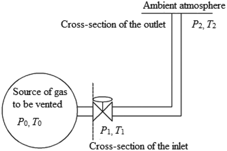
Venting pipeline system model.

Because this study focuses on the flow field of the gas upon being jetted from the outlet of the pipe, the calculation model is simplified to only the section of the venting pipe close to the outlet. Figure 2 shows the simplified computational domain. Considering that the gas flow rate is relatively high at the outlet, the computational domain is increased by 4 m upward along the radial direction of the venting pipe and 10 m along the axial direction of the venting pipe. A structured grid is used and grid encryption is performed inside the sound source plane (Figure 3). The length of the vent pipe is 200 m, The venting pipe has a diameter of 160 mm, an inlet pressure of 0.301 MPa and an inlet temperature of 292 K. The speed of sound in natural gas is 450 m/s. Thus, the venting rate is 225 m/s for an Ma of 0.5. The outlet pressure is the same as the atmospheric pressure (101.325 kPa). The outlet temperature is 280 K. The boundary of the outlet of the venting pipe is equal to the pressure outlet. The left, upper and lower boundaries of the computational domain are equal to the pressure at far-field boundaries. The right boundary of the computational domain is equal to the pressure outlet. The flow simulation was performed with LES.

Figure 2.

Computational domain and boundary conditions.

Figure 3.

Computational domain grid generation.

Figure 4 shows the velocity contours predicted by the simulation. Figure 4 clearly shows that the velocity remains the same within a distance at 6.8 times the diameter of the venting pipe (6.8 D) from the outlet of the pipe, which is the potential core of the jet. The motion of the flow is most intense within this section, which is the main area where the noise is produced.

Figure 4.

Steady velocity contours of the jet flow from the venting pipe.

The section between 6.8 D and 15 D away from the outlet of the venting pipe is the transition section of the jet flow. The movement of the jet flow in this section is relatively complex. However, overall, the difference between the momentum of the jet flow and the momentum of the atmosphere in this section is significantly lower than that in the core section of the potential flow. Therefore, the jet flow rate and turbulent flow intensity both gradually decrease as the distance from the outlet of the pipe increases. In addition, noise transforms from high-frequency noise to low-frequency noise in this section. The section of the jet flow further than 15 D from the outlet of the pipe is its main section. The jet flow rate and turbulent flow intensity decrease more gradually in the main section compared to the transition section, and the majority of noise produced in the main section is low-frequency noise.

Within the main section of the jet flow, the time-averaged values of the flow field are extremely similar, which can be observed in Figure 4. The whole velocity contour curves exhibit a semi-arc shape. The shape of the velocity contours downstream of the jet flow is basically similar to the contours upstream of the jet flow, although the velocity contour on each cross-section of the downstream is slightly expanded compared to the immediately preceding layer. These similarities are reflected in physical parameters such as temperature, speed, and material concentration.

Figure 5 shows the turbulence energy vector diagram of the jet flow from the venting pipe. The turbulence energy of the jet flow remains constant within a certain axial distance after the gas is jetted from the venting pipe, whereas the turbulence energy is relatively high at the two outer sides of the core section of the potential flow, which indicates that the turbulence energy experienced by the gas is highest within this section. The turbulence energy gradually decreases along the axial direction, regardless of whether a point is within the core section or at the outer sides of the potential flow. In addition, the gas flow disturbance spreads out and decreases as the distance in the axial direction increases.

Figure 5.

Turbulent kinetic energy vector diagram of the jet flow (m²/s²).

Figure 6 shows the temperature vector diagram of the jet flow from the venting pipe. The jet flow temperature is 280 K at the outlet of the pipe and gradually increases as the jet flow develops until reaching the atmospheric temperature. Because the pressure inside the venting pipe decreases relatively in a significant way and the temperature at the outlet of the pipe is relatively low, natural gas hydrates can form very easily. This factor should be fully taken into consideration when designing a muffler to avoid a muffler design with an overly small outlet diameter that can lead to blockages.

Figure 6.

Temperature vector diagram of the jet flow (K).

Noise analogy model (FW–H)

In 1969, Ffowcs Williams and Hawkings successfully expanded the application of Lighthill’s acoustic wave equation to study noise sources while considering the effect of moving solid walls using the generalized function method. The FW–H equation is as follows

\begin{matrix} \frac{1}{a_{0}^{2}} \frac{\partial^{2} p'}{\partial t^{2}} - \nabla^{2} p' = \frac{\partial^{2}}{\partial x_{i} \partial x_{j}} {T_{ij} H (f)} \\ - \frac{\partial}{\partial x_{i}} {[P_{ij} n_{j} + ρ u_{i} (u_{n} - v_{n})] δ (f)} \\ + \frac{\partial}{\partial t} {[ρ_{0} v_{n} + ρ (u_{n} - v_{n})] δ (f)} \end{matrix}

(1)

In which, $p'$ is the far-field sound pressure in $Pa$ , $a_{0}$ is the local speed of sound in $m / s$ , $ρ_{0}$ is the density of the flowing medium in $kg / m^{3}$ , $u_{n}$ is the fluid velocity component in $m / s$ , $v_{n}$ is the surface velocity component in $m / s$ , $T_{ij}$ is the Lighthill stress tensor in $Pa$ , $δ_{ij}$ is the Kronecker symbol, $δ (f)$ is the Dirac function, and $H (f)$ is the Heaviside function.

The FW–H model solves the flow and wave equations through decoupling. The FW–H equation used in ANSYS Fluent is based on Lighthill’s acoustic analogy theory. By solving the FW–H equation, the noise sound field of monopole, dipole, and quadrupole sound sources can be obtained.^24–27

Jet noise produced by venting pipes is a quadrupole sound source. To obtain the frequency spectral characteristics of the SPL of the far-field sound field and the noise transmission pattern in the free space, the FW–H acoustic analogy model is used to calculate the sound field.

Analysis of noise produced by a venting system

Simulation of the radiated sound field of the jet flow from a venting pipe

Generally, the venting pipe at a natural gas station is placed at a relatively high location, and there is some distance between the outlet of the venting pipe and the ground. To understand how the jet noise is transmitted to the ground as well as at the noise transmission pattern, it is necessary to simulate the radiated sound field of the jet noise. Based on the jet flow field simulation results, a numerical prediction of the jet noise is made using the FW–H method. The computational domain is the same as the one previously used in the flow field simulation. The sound source plane in the computational domain starts at the outlet of the venting pipe and expands gradually. In addition, the sound source plane has a diameter four times the outlet diameter of the venting pipe (D), a length of 6.8 D in the straight-line section and a diameter of 8 D in the expanded section.

The extreme value of the noise frequency $f = (1 / 2 Δ t)$ calculated using ANSYS Fluent is limited by the time step. Because the range of frequencies that can be heard by the human ear is between 20 and 20,000 Hz, the time step is $Δ t = 2.5 \times 10^{- 5} s$ , so the corresponding limit frequency is 20,000 Hz. The noise model is started after the unsteady calculation of the flow field has been performed for 4000 steps. The results are automatically saved after iterating every 50 steps.

The FW–H method can predict the far-field sound pressure, that is, the sound-monitoring points can be located anywhere outside the computational domain. With a venting pipe 20-m tall, the monitoring points are set at intervals of 5 m in the axial (x) and radial (y) directions of the gas jet flow with the outlet of the venting pipe as the origin. Figure 7 shows the location and coordinates of each monitoring point.

Figure 7.

Schematic diagram of the noise-monitoring points.

The grid independent verification had been done to eliminate the calculation error caused by the number of grids. Two monitoring points (D1, D7) were selected to compare the simulation results under different grid conditions.

Using the pre-processing software ICEM, the grid information was shown in Table 1.

Table 1.

The information of the grids.

	I	II	III	IV
Node number	150146	104310	53798	28696
Mesh number	153621	106583	54827	29471
Minimum area (m²)	2.162144e–03	5.161285e–03	1.000000e–02	1.000000e–02
Maximum area (m²)	1.685715e–02	2.532768e–02	5.091000e–02	6.379795e–02

According to the calculation results of the above four kinds of mesh, using the grid number as the independent variable, the sound pressure as variable, the maximum, minimum, and average sound pressure at the monitoring points D1 and D7 were shown in Figure 8.

Figure 8.

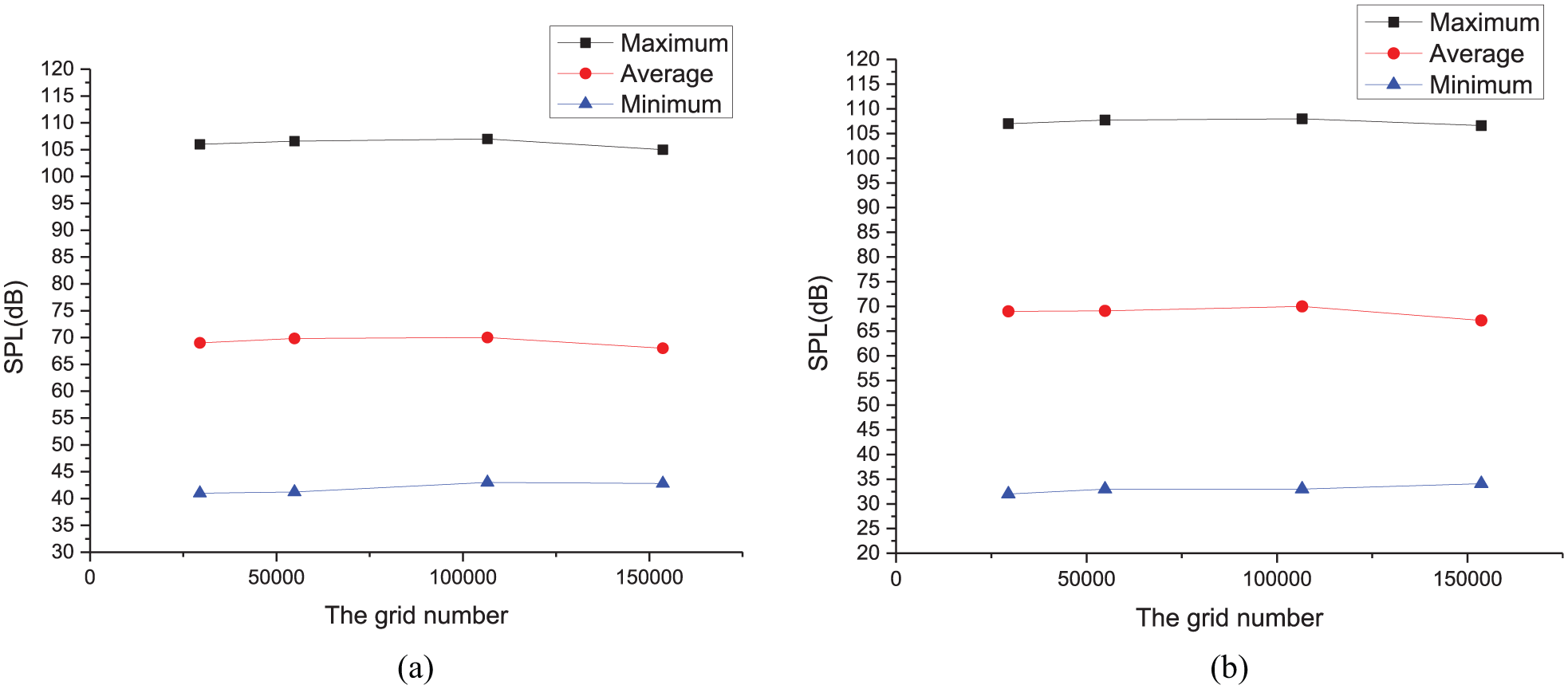
SPL distribution with different grid number: (a) SPL distribution at D1 and (b) SPL distribution at D7.

As shown in Figure 8, the maximum, average, and minimum values of sound pressure fluctuate slightly with the change of the number of grids, but the change value was very small. In order to save the calculation cost and save the calculation time, the number of grid in this article was controlled at about 50,000.

Figure 9 shows the spectra of the sound pressure at various monitoring points at an axial distance of 5 m and different radial distances from the outlet of the venting pipe.

Figure 9.

SPL distribution at various monitoring points at an axial distance of 5 m and different radial distances from the outlet of the venting pipe: (a) SPL distribution at (–5, 0), (b) SPL distribution at (–5, 5), (c) SPL distribution at (–5, 10), (d) SPL distribution at (–5, 15), (e) SPL distribution at (–5, 20), (f) SPL distribution at (–5, 25), and (g) SPL distribution at (–5, 30).

Figure 9 shows that the SPL distribution and variation trend are basically the same between various monitoring points. The SPL is relatively high in the low-frequency range (0–1000 Hz) and decreases to an average level in the frequency range of 1000–4000 Hz. The SPL at points A1, A2, A3, A4, A5, A6, and A7 reaches its peak values (115.53, 118.85, 116.8, 116.21, 115.37, 114.48, and 113.61 dB, respectively) at 256, 165, 238, 206, 206, 206, and 238 Hz, respectively. Thus, the peak SPLs at the monitoring points occur at similar frequencies.

From the aforementioned spectra, the venting noise is a typical low-frequency noise, that is, the SPL of the venting noise is relatively high in the low-frequency range. Different from low-frequency noise, high-frequency noise rapidly attenuates as the distance increases or upon encountering an obstacle. For example, the SPL of high-frequency noise produced by a point sound source decreases by 6 dB for every 10-m increase in the distance. In comparison, low-frequency noise attenuates very slowly and consists of relatively long sound waves. Low-frequency noise can easily penetrate obstacles, travel long distances, and penetrate walls to reach people’s ears.

To visually observe the variation trend of the SPL at each monitoring point, the average, maximum SPLs at the monitoring points at an axial distance of 5 m and different radial distances from the outlet of the venting pipe (points A1–A7) are plotted as broken lines in Figure 10.

Figure 10.

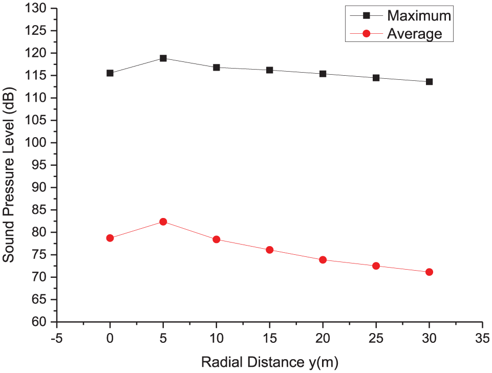
Curves of the sound pressure at an axial distance of 5 m from the outlet of the venting pipe with radial distance.

Figure 10 shows that for the same axial distance, the average SPL changes insignificantly with radial distance and basically fluctuates approximately 80 dB. The average SPL increases slightly as the radial distance increases between 0 and 5 m and then decreases slowly as the radial distance increases beyond 5 m. The maximum SPL is approximately 115 dB and changes insignificantly. The minimum SPL changes irregularly and has the lowest value at a radial distance of 20 m from the outlet of the venting pipe.

Similarly, the maximum, average, and minimum SPLs at other monitoring points are shown in Figures 11 and 12. Figure 11 shows that the average SPL decreases as the axial distance increases, which is mainly because sound waves undergo attenuation during the transmission process.²⁸

Figure 11.

Average SPLs at the monitoring points at different axial and radial distances from the outlet of the venting pipe.

Figure 12.

Maximum SPLs at monitoring points for different axial and radial distances from the outlet of the venting pipe.

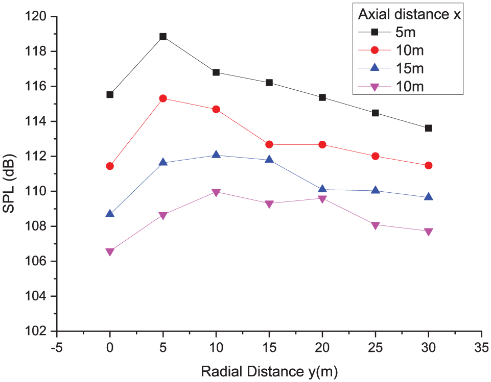
The average SPL varies between the monitoring points at the same axial distance but different radial distances from the outlet of the venting pipe. This behavior is the result of radiated sound intensity varying in different directions when sound is transmitted outwardly, which is the so-called sound intensity directivity. Research has shown that directivity is closely related to sound frequencies. As the sound frequency increases, the directivity increases. Therefore, some low-frequency noise has very low directivity²⁹ because the time needed by a sound wave to travel from the sound source to the receiving point varies between sound waves with different frequencies. As a result, sound waves will interfere with one another, which is then manifested as directivity. Based on Figure 11, the average SPL is the greatest at an axial distance of 5 m and a radial distance of 5 m from the outlet of the venting pipe, that is, the directivity of the sound source is the highest at this location. Similarly, the highest value of the average SPL at an axial distance of 10, 15, and 20 m from the outlet of the venting pipe occurs at a radial distance of 10, 10, and 15 m, respectively, from the outlet of the venting pipe.

The maximum SPLs at the monitoring points are plotted as broken lines in Figure 12. Based on Figure 12, it can be concluded that for the same radial distance condition, the maximum SPL decreases as the axial distance increases; the highest value of the maximum SPL at the point, that is, an axial distance of 5, 10, 15, or 20 m from the outlet of the venting pipe occurs at a radial distance of 5, 5, 10, or 10 m, respectively, from the outlet of the venting pipe.

The general hearing protection standard stipulated in the Emission Standard for Industrial Enterprises Noise at a Boundary³⁰ of China and the US National Institute for Occupational Safety and Health states that continuous exposure to 90 dB of noise should not exceed 8 h and continuous exposure to 95 dB of noise should not exceed 4 h, otherwise there is a 100% probability of developing hearing impairment. Therefore, the maximum SPL of noise produced during a direct natural gas venting process should not exceed 90 dB. Figure 12 clearly shows that the SPL of the noise at each monitoring point already considerably exceeds the national standard.

Effect of the Ma at the outlet on the venting noise

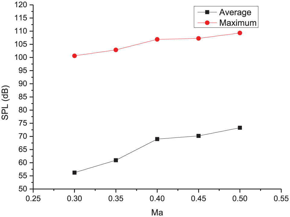
During the venting process, the flow rate at the outlet of the venting pipe changes constantly. To study the effect of the Ma at the outlet on the venting noise, simulations are performed with Ma values of 0.5, 0.45, 0.4, 0.35, and 0.3 at the outlet to compare the SPL for different Ma conditions at the outlet. Based on the analysis in the previous section, when the outlet of the venting pipe is 20 m above the ground, the radiated SPL is highest on the ground 15 m away from the venting pipe. Therefore, the point located at (–20, 15) is selected as the monitoring point. A comparative analysis is performed on the SPL at this monitoring point for different Ma conditions at the outlet, while other conditions remain the same.

When $Ma = 0.5$ , the flow rate at the outlet is 225 m/s. Based on Figure 13, the average SPL at the monitoring point located at (–20, 15) is 73.29 dB, and the SPL reaches its maximum (109.31 dB) at approximately 208.76 Hz. The SPL remains relatively high in the low-frequency range (0–500 Hz), generally decreases in the frequency range of 500–2000 Hz and slowly increases while fluctuating approximately 70 dB in the frequency range of >2000 Hz.

Figure 13.

SPL distribution when $Ma = 0.5$ .

Similarly, the average, maximum, and minimum SPLs for different Ma conditions can be observed in Figure 14.

Figure 14.

Behavior of the SPL versus Ma.

The following conclusions are obtained by analyzing Figure 14: The maximum and average SPLs at the same monitoring point both decrease as the Ma at the outlet of the venting pipe decreases. Therefore, under actual working conditions, noise can be controlled by controlling the flow rate at the outlet of the venting pipe within a reasonable range.

Design of a muffler

Based on the analysis of the frequency spectrum of the radiated noise produced by a venting pipe, noise produced during a gas venting process at a natural gas station is low-frequency noise. In this section, a 20-m tall upright venting pipe is studied with a monitoring point at (–20, 15). The SPL at this point reaches its maximum at 209 Hz. Based on the frequency spectrum of the SPL at this monitoring point, the focused frequency range of noise reduction by a muffler is set to 0–750 Hz.

Structural design of an expansion-chamber muffler

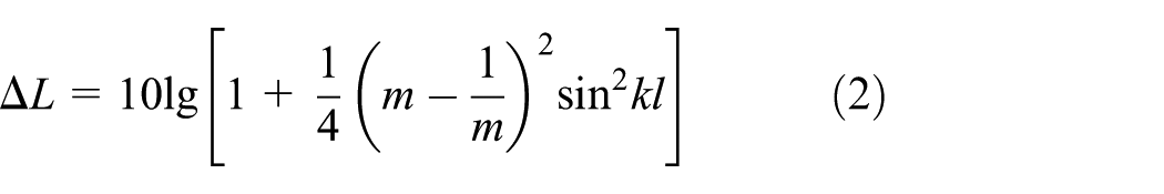
The noise reduction performance of an expansion-chamber muffler depends on the expansion ratio (m) and the length of the expansion chamber (l). The amount of noise reduced by a single-section expansion-chamber muffler can be calculated using the following equation³¹

Δ L = 10 \lg [1 + \frac{1}{4} {(m - \frac{1}{m})}^{2} si n^{2} kl]

(2)

where $Δ L$ is the amount of noise reduced, dB; $m$ is the expansion ratio (the ratio of the cross-section of the expansion chamber to the cross-section of the gas flow channel); $k$ is the wavenumber ( $k = (2 π / λ) = (2 π f / c) = (ω / c)$ in which different $k$ values correspond to different frequencies); and $l$ is the length of the expansion-chamber muffler, m.

Based on equation (2), $Δ L$ is a periodic function of $kl$ . The maximum value of $Δ L$ occurs when $si n^{2} kl = 1$ , at which point $kl = π / 2$ and $l = λ / 4$ , that is, the maximum amount of noise reduced occurs when l equals $1 / 4$ of the wavelength or an odd number of times $1 / 4$ of the wavelength. Thus, equation (2) can be rewritten as

Δ L_{m} = 10 \lg [1 + \frac{1}{4} {(m - \frac{1}{m})}^{2}]

(3)

Based on equation (3), the amount of noise reduced is mainly determined by m. The amount of noise reduced increases as m increases. When $m > 5$ , equation (3) can be approximated by the following equation

Δ L_{m} = 20 \lg \frac{m}{2} = 20 \lg m - 6

(4)

As m increases, the amount of noise reduced increases. The upper cut-off frequency of noise that can be effectively reduced by an expansion-chamber muffler can be determined equation (4),³² as follows

f_{up} = 1.22 \frac{c}{D}

(5)

where c is the speed of sound, m/s; and D is the cross-sectional diameter of the expansion chamber, m.

Based on equation (5), a larger D results in a lower frequency for the upper cut-off frequency of noise reduced, a smaller frequency range of noise that the muffler can reduce and a smaller m. However, for a smaller D, the amount of sound reduced by the muffler is smaller. Therefore, there is a conflict between an increase in the upper cut-off frequency of noise that can be reduced and an increase in the amount of sound reduced. A reasonable m should be selected to achieve the optimum noise reduction results.

Because the SPL of the outlet noise is relatively high in the frequency range of 0–1000 Hz, 1000 Hz is set as the upper cut-off frequency of the noise reduced by a muffler. The diameter of the expansion chamber is calculated using equation (5)

D = \frac{1.22 c}{f_{up}} = \frac{1.22 \times 450}{1000} = 0.549 m

(6)

To achieve the maximum amount of noise reduced, l should meet the requirements of the following equation

l = \frac{c}{4 f}

(7)

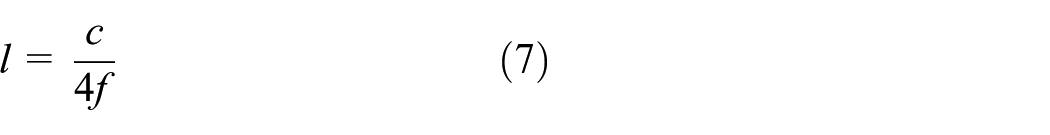
Based on equation (7), the frequency of noise that can be reduced by a muffler can be altered by changing l. An increase in l results in a decrease in the frequency of noise reduced by the muffler. Based on the frequency spectrum, the SPL reaches its maximum at 209 Hz. However, another small peak SPL also appears at 385 Hz. Therefore, a double-cavity expansion-chamber structure is considered. The length of each cavity is calculated using equation (7)

l_{1} = \frac{c}{4 f_{1}} = \frac{450}{4 \times 209} = 0.538 m

l_{2} = \frac{c}{4 f_{2}} = \frac{450}{4 \times 385} = 0.292 m

The major disadvantage of a single-section expansion-chamber muffler is that it can only reduce sound waves with specific frequencies. When $l = 1 / 2$ or an integer number of times the wavelength, the amount of noise reduced is zero. To eliminate this disadvantage, ducts are generally inserted into the expansion chamber. A $l / 2$ -long duct and a $l / 4$ -long duct are inserted at the inlet and outlet, respectively. A theoretical analysis has shown that an insertion of an $l / 2$ -long duct can eliminate sound waves with a frequency of an odd number of times $l / 2$ , and an insertion of a $l / 4$ -long duct can eliminate sound waves with a frequency an even number of times $l / 2$ .^33–35 There is a 180° phase difference between a sound wave transmitted forward and a sound wave reflected after encountering an interface; however, these two sound waves have the same amplitude. Therefore, these two sound waves have opposite phases and interfere with one another. This method is used to eliminate sound waves with various frequencies.

Figure 15 shows the three-dimensional (3D) structure of an improved expansion-chamber muffler designed based on the calculation results. Figures 16 and 17 show the dimensions of the muffler in detail.

Figure 15.

Structural diagram of an improved expansion-chamber muffler.

Figure 16.

Dimensions of the muffler.

Figure 17.

Locations of the ducts inside the muffler.

The noise reduction effect of a muffler can be negatively affected if a high-flow-rate gas flow rapidly rushes out of the muffler after entering it. To prevent this result, the inlet and outlet of the chamber are placed at staggered locations relative to one another, and ducts 1 and 2 share the same central axis. A baffle is inserted inside the chamber to separate the chamber into two cavities. To withstand the impact of a high-flow-rate gas flow, a material with relatively high strength should be used to fabricate the baffle.

Numerical simulation of the muffler

To verify the noise reduction effect of the expansion-chamber muffler designed in this study, a numerical simulation is performed. Grid generation is performed using ANSYS ICEM. Considering the computational cost, an unstructured grid is used. There are a total of approximately 600,000 grid cells. Figure 18 shows the generated grid for the computational domain of the muffler and the sound field outside the muffler. Figure 19 shows the generated grid of the inside of the muffler.

Figure 18.

Generated grid of the computational domain of the muffler and the sound field outside the muffler.

Figure 19.

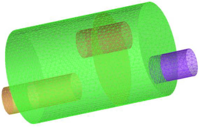
Generated grid of the inside of the muffler.

A pulse sound pressure spectrum is predicted using ANSYS Fluent, which is converted to a sound pressure frequency spectrum using the fast Fourier transform (FFT). The monitoring point at which the radiated sound pressure reaches its maximum value (i.e. the point located at (–20, 15)) is selected for analysis.

Figure 20 shows that before the muffler is installed, the SPL is relatively high in the frequency range of 0–1000 Hz, decreases as the frequency increases in the frequency range of 1000–2000 Hz, and insignificantly fluctuates around the average level in the frequency range of >2000 Hz. Overall, the SPL considerably exceeds the standard in the low-frequency range. In comparison, Figure 21 shows that after the muffler is installed at the outlet of the venting pipe, the SPL decreases significantly. In particular, in the low-frequency range, the maximum SPL at the monitoring point decreases from the initial 109.31 to 89.95 dB, a nearly 20-dB decrease; in addition, the average SPL at the monitoring point also decreases from 73.29 to 60.88 dB, which indicates that the expansion-chamber muffler designed in this study is highly effective in reducing noise.

Figure 20.

Frequency spectrum of the sound pressure at the monitoring point when no muffler is used.

Figure 21.

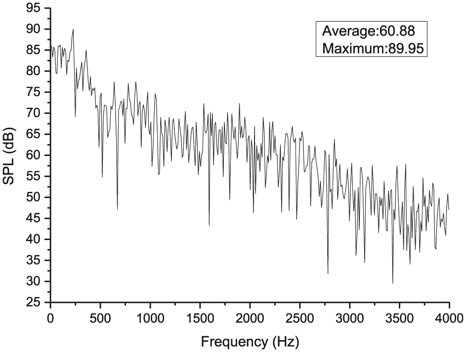
Frequency spectrum of the sound pressure at the monitoring point when the muffler is used.

The noise reduction effect of the muffler can be more clearly observed in Figure 22. The main goal is to reduce low-frequency noise under this working condition. Therefore, only the low-frequency range (1–1000 Hz) in which the SPL is relatively high is selected for comparison. At the same frequency, the SPL decreases by 15.01 dB on average and up to 37.9 dB, which further demonstrates that the expansion-chamber muffler designed in this study is effective in reducing low-frequency noise.

Figure 22.

Comparison of the SPL in the low-frequency range when the muffler is installed to when the muffler is not installed.

In addition, ideal noise reduction results are achieved at other monitoring points on the ground by using the muffler. Table 2 shows the comparison of the SPL before and after the installation of the muffler. While there are differences in the frequency range of noise reduced by the muffler and the extent to which the SPL decreases between different monitoring points, a relatively large amount of noise in the low-frequency range, generally ranging from 20 to 40 dB, is reduced. Furthermore, the maximum SPL is controlled below 90 dB.

Table 2.

Comparison of the SPL at each monitoring point on the ground.

Monitoring point number	Change in the sound pressure (dB)
	Maximum		Minimum		Average
	Without themuffler	With themuffler	Without themuffler	With themuffler	Without themuffler	With themuffler
D1	106.58	89.43	41.22	20.67	69.83	60.54
D2	108.66	89.60	43.85	31.69	71.22	61.30
D3	109.97	90.14	44.87	23.22	72.94	61.35
D4	109.31	89.95	47.16	29.56	73.29	60.88
D5	109.60	89.36	51.61	24.37	72.12	60.97
D6	108.10	88.57	37.72	28.98	70.33	60.15
D7	107.73	87.70	32.99	22.15	67.09	59.40

The following conclusions are drawn from Table 2.

The expansion-chamber muffler designed in this study can effectively reduce low-frequency jet noise produced by a venting pipe. The muffler can effectively reduce the SPL by 10–40 dB.

The muffler designed in this study produces varying noise reduction results for noise at different frequencies. However, this muffler is particularly effective in reducing low-frequency noise.

Conclusion

The SPL of jet noise produced during a gas venting process at a natural gas storage and transmission station can be greater than 110 dB. Noise at this level can easily cause severe mental harm to personnel working at the station and residents living nearby. Therefore, noise prevention and control measures must be implemented.

Based on the analysis of the frequency spectral characteristics of radiated noise produced during a venting process, an expansion-chamber muffler is designed to reduce noise. After an evaluation, it is found that the muffler designed in this study is effective at reducing low-frequency noise and the SPL by 10–40 dB. In addition, with this muffler, the maximum SPL is controlled below 90 dB and the average SPL is controlled at approximately 60 dB. Furthermore, the pressure resistance loss ratio resulting from the use of the muffler designed in this study is 22.6%, which meets the aerodynamic performance requirements for venting pipes during a gas venting process.

Footnotes

Handling Editor: Hongfang Lu

Declaration of conflicting interests

The author(s) declared no potential conflicts of interest with respect to the research, authorship, and/or publication of this article.

Funding

The author(s) disclosed receipt of the following financial support for the research, authorship, and/or publication of this article: This work was supported by the special fund of Key Technology project of safety production of major accident prevention and control (sichuan-0002-2016AQ, sichuan-0013-2016AQ) and open fund project of Sichuan Key Laboratory of Oil and Gas Fire Fighting (YQXF201603).

ORCID iD

Enbin Liu

References

Gang

Feng

. Talking about the measure of environmental pollution and public hazard. Sci Technol Forum 2015; 5: 1–13.

Peng

Liu

Xian

et al . Dynamic simulation of an underground gas storage injection-production network. J Environ Biol 2015; 36: 799–806.

Liu

Wen

Peng

et al . A study of the numerical simulation of water hammer with column separation and cavity collapse in pipelines. Adv Mech Eng 2017; 9: 1–13.

Gang

Wu.

Structural vibration of ocean engineering and the calculation of acoustic characteristics. Master’s Degree Thesis, Shanghai Jiaotong University, Shanghai, China, 2008.

Jun

Yunjian

Debin

Huang

. Harm and control of industrial noise. Commun Sci Technol 2012; 6: 106–107.

Chengwu

Fan

Shijie

. Technology research on safety venting system of Puguang gathering station. Safe Heal Environ 2013; 5: 19–21.

Liu

Yang

Optimal energy consumption analysis of natural gas pipeline. Sci World J 2014; 2014: 506138.

Lighthill

MJ.

On sound generated aerodynamically. P Roy Soc Lond A: Mat 1952; 211: 564–587.

Curle

The influence of solid boundaries upon aerodynamic sound. P Roy Soc Lond A: Mat 1955; 231: 505–514.

10.

Ffowcs Williams

Hawkings

. Sound generation by turbulence and surfaces in arbitrary motion. P Roy Soc Lond A: Mat 1969; 264: 321–342.

11.

Goldstein

ME.

Aeroacoustics. New York: McGraw-Hill Book Company, 1976, pp.159–169.

12.

Freund

Lele

Moin

. Direct simulation of a Mach 1.92 jet and its sound field. In: 4th AIAA/CEAS aeroacoustics conference, Toulouse, 2–4 June 1998, pp.98–119. Reston, VA: AIAA.

13.

Freund

. Noise sources in a low Reynolds number turbulent jet at Mach 0.9. J Fluid Mech 2001; 438: 277–305.

14.

Stromberg

Mclaughlin

Troutt

TR.

Flow field and acoustic properties of a Mach number 0.9 jet at a low Reynolds number. J Sound Vib 1980; 72: 159–176.

15.

Piomelli

Streett

Sarkar

On the computation of sound by large-eddy simulation. J Eng Math 1997; 32: 217–236.

16.

Seror

Sagaut

Bailly

et al . On the radiated noise computed by large-eddy simulation. Phys Fluids 2001; 13: 476–487.

17.

Zhao

Frankel

Mongeau

Effects of spatial filtering on sound radiation from a subsonic axisymmetric jet. AIAA J 2000; 38: 2032–2039.

18.

Mankbadi

Hayder

Povinelli

LA.

Structure of supersonic jet flow and its radiated sound. AIAA J 1994; 32: 897–906.

19.

Lyrintzis

Mankbadi

RR.

Prediction of the far-field jet noise using Kirchhoff’s formulation. AIAA J 1996; 1: 1–4.

20.

Gamet

Estivalezes

JL.

Application of large-eddy simulation and Kirchhoff method to jet noise prediction. AIAA J 1998; 36: 2170–2187.

21.

Zhao

Frankel

Mongeau

Large eddy simulation of sound radiation from subsonic turbulent jets. AIAA J 2001; 39: 1469–1477.

22.

Bogey

Bailly

LES of a high Reynolds, high subsonic jet: effects of the inflow conditions on flow and noise. AIAA paper 2000–3170, 2000.

23.

Bogey

Bailly

LES of a high Reynolds, high subsonic jet: effects of the subgrid modellings on flow and noise. AIAA paper 2003–3557, 2003.

24.

Fluid products business unit of ANSHIYATAI. ANSYS Fluent the solutions of aero aerodynamic noise. Aeronaut Manuf Technol 2012; 9: 103–104.

25.

Liu

Yan

Peng

SB.

Noise silencing technology for manifold flow noise based on ANSYS fluent. J Nat Gas Sci Eng 2016; 29: 328.

26.

Liu

Yan

Peng

et al . Large Eddy Simulation and FW-H acoustic analogy of flow-induced noise in elbow pipe. J Comput Theor Nanos 2016; 12: 2866–2873.

27.

Liu

Tan

Peng

A CFD simulation for the ultrasonic flow meter with a header. TEH VJESN 2017; 24: 1797–1801.

28.

Wei

Yan

. Design of venting system of gas transmission station. Petrol Eng Constr 2012; 6: 39–43.

29.

Chao

Peilin

Zhang

Huaiguang

Wang

. Numerical simulation and experimental study of non-linear sound field of ultrasonic abrasive grain sensor. Lubr Seal 2014; 7: 11–15.

30.

Yunlong

Gao

. Talking about the characteristic of EASE database speaker. Sound Technol 2006; 12: 22–25.

31.

GB 12348:2008. Environmental noise emission standard for industrial enterprises.

32.

Jian

Yan

. Study on optimization design and performance analysis method of muffler for small oxygen making. Master Thesis, Southeast University, Dhaka, Bangladesh, 2009.

33.

Selamet

Denia

Besa

AJ.

Acoustic behavior of circular dual-chamber mufflers. J Sound Vib 2003; 265: 967–985.

34.

Yong

Chen

Peng

Hao

. Mechanical performance experiments on rock and cement, casing residual stress evaluation in the thermal recovery well based on thermal-structure coupling. Energ Explor Exploit 2017; 35: 591–608.

35.

Yong

Tao

Calculation and analysis of the first interface micro-gaps of the thermal production wells. Adv Mech Eng 2017; 9: 1–9.

Noise-silencing technology for upright venting pipe jet noise

Abstract

Keywords

Introduction

Venting system model

Analysis of the flow field of a venting system

Noise analogy model (FW–H)

Analysis of noise produced by a venting system

Simulation of the radiated sound field of the jet flow from a venting pipe

Effect of the Ma at the outlet on the venting noise

Design of a muffler

Structural design of an expansion-chamber muffler

Numerical simulation of the muffler

Conclusion

Footnotes

Declaration of conflicting interests

Funding

ORCID iD

References