Sage Journals: Discover world-class research

Abstract

This study experimentally and numerically investigates the performance of a circular cylinder with a spiral grooved surface in terms of reducing wind drag. Its application in the overhead high-power conductor plays a vital role, especially in typhoon conditions. Wind tunnel tests have shown that at the critical Reynolds number (Re), the coefficients of wind drag decrease to a greater extent in a spiral grooved cylinder than in a smooth circular one. Moreover, a cylinder with a shallow groove and a small number of spirals could reduce the coefficient of drag in typhoon conditions. To gain an insight into the underlying fluid mechanism, a large-eddy simulation of turbulent flow from a critical to a super-critical Re has been carried out to approximate the flow separation and turbulent eddies over the spiral grooved cylinder. The results of the wind tunnel test have been used as a benchmark for the numerical results. The flow characteristics have been established about the near-wall flow separation and far wake flow, the pressure coefficient, the skin-friction coefficient, drag coefficient, and Q-criterion field.

Keywords

CFD grooved cylinder large-eddy simulation OpenFOAM

Introduction

The spiral grooved cylinder has many applications, including as the low wind-pressure conductor.¹ The conventionally used high-power conductor is the so-called aluminum conductor with a steel-reinforced (ACSR) core. Its cross-section and outer profile are shown in Figure 1(a) and (b). Figure 1(c) and (d) show an overhead conductor recently developed by Eguchi et al.^2,3 Semi-circular grooves are spirally fabricated on the surface of the conductor. Its profile is inspired by the dimpled surface of a golf ball. As it moves in the air at high speed, flow separation occurs on the surface of the ball. The laminar flow moves leeward and clings to the surface before the separation point. The vortices are detached after this point and turbulent flow is formed downstream. The flow slows down in the wake and creates a region of considerably lower pressure. A large drag force arises due to the turbulence. The dimples on the surface of the ball can delay the flow separation, which leads to the formation of less vortex region in the wake.⁴ As a result, there is less drag on the ball, which is why a golf ball can travel farther at high speeds than one with a smooth surface.

Figure 1.

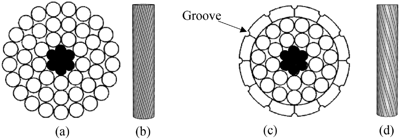
A conventional overhead power conductor: (a) cross-sectional view and (b) side view. The inner part is a steel-reinforced (ACSR) core, the outer aluminum wires wrap in spiral. A recently developed conductor by Eguchi et al.²: (c) cross-sectional view and (d) side-view. Twelve semi-circular grooves are engraved in the outmost layer.

Grooves on an overhead conductor serve the same purpose as the dimples fabricated on a golf ball. Scientists have proved that both grooved surface and the dimpled can cause drag reduction.⁵ These can both delay the flow separation and result in a smaller wake region, causing a lower drag than the smooth cylinders.^6–8 The results of wind tunnel tests have shown that such a conductor performs a lower drag by 32% compared with the conventional conductor at Re = 10⁵ in the typhoon condition.² There has been an equivalent reduction in drag in field trials.³ Furthermore, such a conductor can better suppress swing, noise, and vibrations.^3,9 Matsumura et al.¹⁰ carried out a field test to verify the performance of a low wind-pressure conductor. A reduction of 5% in the maximum tension was noted compared to an ordinary conductor when the wind speed exceeded 18–20 m/s. Studying the flow mechanism around the grooved cylinder is crucial to determine its effectiveness in reducing wind drag.

A parametric study was conducted by Liu et al.¹² through a wind tunnel test in order to find the groove pattern that minimizes wind drag. The tested aluminum wires were the conventional ASCR JLX1/G1A (DFY)-675/45 with a diameter of 33.75 mm. The effect of the groove angles (see Figure 2(a)) on wind drag was studied experimentally at a wind speed range of 20–70 m/s. They found that the groove angle θ at 90° yielded the highest reduction in drag. The helical angle β (shown in Figure 2(a)), groove angle θ, pitch distance h_p, and the number of grooves in the circumferential direction of a grooved cylinder are experimentally examined through wind tunnel tests.¹³ According to their findings, the drag coefficients are sensitive to Re, and decrease only in the flow range of the critical Re compared to a cylinder with smooth walls. Cactus-like surface pattern has been applied to a cylindrical cylinder and longitudinal grooves of varying depths have been tested in a wind tunnel. Such a surface yields a lower fluctuating side force than a cylinder with smooth walls.¹⁷ The quick pressure recovery on the sides of the cylinder results in less wind drag.

Figure 2.

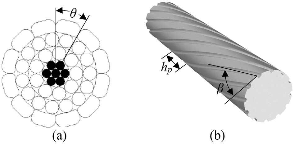
Schematic view of (a) the groove angle θ between two grooves, and (b) the helical groove angle β and groove pitch distance h_p.¹²

Although data on the aerodynamic performance of spiral grooved cylinders can be obtained from wind tunnel tests, the flow separation and structure of the vortex are challenging to visualize and measure. Moreover, flow physics is complex and sensitive to the Re.¹⁴ The regimes for turbulent flow past a circular cylinder with a smooth wall are classified as the subcritical, critical, supercritical, and transcritical ranges of Re with respect to the pattern of flow separation and drag force.^11,15 Numerical methods play an important role in exploring such flow behaviors over the body of the cylinder. To predict turbulent flow, large-eddy simulations (LES) are more accurate than the Reynolds-averaged Navier–Stokes (RANS) equations in terms of large-scale turbulence structures and dynamic force fluctuations.^16,19,21 However, they are computationally expensive because a very fine mesh and small time steps are required to capture the near-wall flow structure. Despite its poor efficiency, a growing number of scientists and engineers are using the LES to run turbulent flow passing blunt bodies owing to recent developments in computing hardware.

The grooved cylinder with a structure analogous to that of a cactus have been numerically examined compared with the surface smoothed cylinder on the wall-pressure fluctuation and the vortices appeared in the wake.^18,20 The V-shaped grooved cavities caused the thicker free shear layer. Cheng et al.²² used the LES method to approximate the turbulent flow field over a straight-grooved cylinder. They compared its properties, in terms of the mean flow, pressure coefficient, skin-friction coefficient, pressure gradient, different near-wall flow patterns, and the critical range of Re for drag, in comparison with those of a smooth cylinder. A significant reduction in drag was observed in the super-critical range of Re.²³ However, to the best of our knowledge, the spiral grooved cylinder has been rarely studied numerically in the literature. For overhead higher-power conductors, it is critical to understand the impact of the grooved cavities on both drag reduction and the wall-pressure fluctuation during their design. This is also the motivation of this research work.

The spiral grooved cylinder is investigated experimentally and numerically in this study. In order to minimize the wind drag, a parametric analysis of groove angle and depth of the groove in the typhoon condition is performed. The occurrence of flow separation from the wall of the cylinder, and the consequent vortex interference and aerodynamics are explored. This paper is organized as follows: the numerical technique of the LES method is introduced in Section 2. The experimental apparatus and setup for a wind tunnel test on the spiral grooved cylinders are described in Section 3. The discussion focuses mainly on the effect of particulars of the grooves on the drag coefficient. The aerodynamics of the spiral grooves and the flow structures predicted using the numerical method are given in Section 4. The conclusions of this study are offered in Section 5.

Experimental setup

The experiment was conducted in a low-speed and closed return wind tunnel at the Nanjing University of Aeronautics and Astronautics. A schematic view of the apparatus for the experiment is presented in Figure 3(a). The range of wind speed for the test was from 5 to 90 m/s. The free-stream turbulence intensity was 0.1%–0.14% which was measured using hot-wire anemometer (CTA). It is the ratio of the standard deviation of mean velocity to mean velocity.³⁴ The favorable value is usually lower than 0.4%. The high value in the test section may trigger incorrect test results due to the high turbulence level in the free stream.³⁵ A 1.36 m long circular cylinder was mounted on a sting at the center of the test section as shown in Figure 3(b). The test section of the tunnel was 3 m wide, 2.5 m high, and 6 m long. The cylinder was made of aluminum. Aerodynamic forces were converted to voltage signals via the balance system located under the floor. The output signal was amplified by the amplifier and recorded by a computer.³⁶ In the experiment, the support sting also created wind drag. The drag on the cylinder was calculated by subtracting the drag on the support sting from the total wind drag on it and the wire. It was assumed that the interaction between the support sting and the cylinder was negligible. This experimental setup is different from that of experiments where the instruments used for measurement are connected directly to the cylinder.^13,36 Additionally, in their experiment, to mitigate the effect of the end wall of the cylinder on C_D, the ends were set very close to the wall of the wind tunnel. In present experiment, the wind tunnel was wide enough and a very long cylinder was used, and thus the effect of the wire ends was insignificant. During the test, the wind speed U ranged from 20 to 70 m/s. The blockage ratio was 2%, so its effect on the drag coefficient and pressure distribution was considered negligible, and blockage correction was not necessary.^14,31

Figure 3.

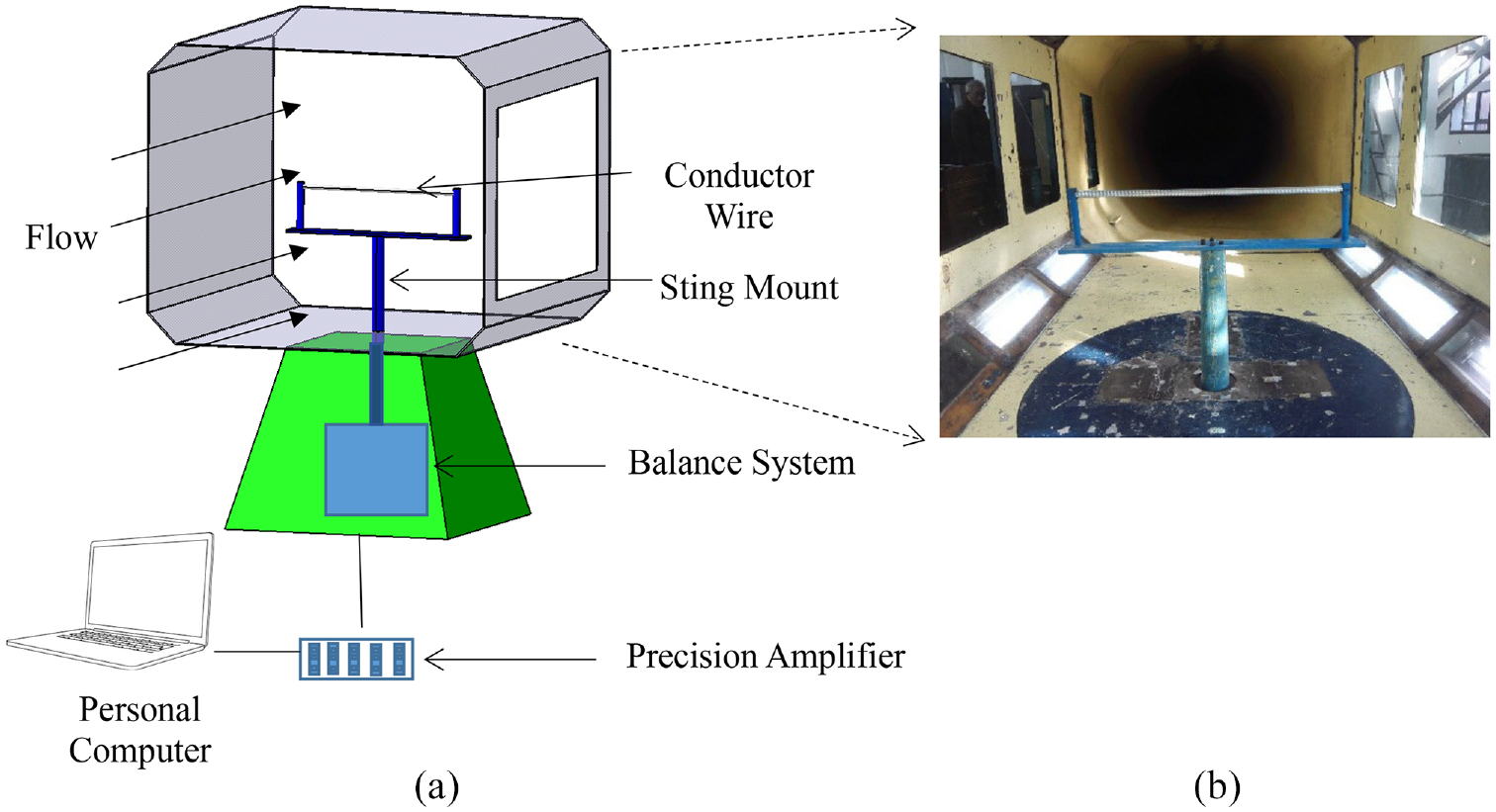
(a) Setup of the wind tunnel test and (b) view of the test section of the wind tunnel.

The configurations of the cross-section of the tested cylinder are presented in Figure 4. R was the outer radius and r was the inner radius of the grooves. A and C were two neighboring peak points, $∠ AOC$ was defined as the groove angle θ, and M was the middle-inner point between A and C. The three points A, M, and C were connected by a non-uniform rational B-spline curve. The groove depth was h (=R − r). Six cylinders with different groove angles θ and depths h were tested, and their particulars are given in Table 1. The diameter of the grooved cylinder D (=2R) was 34.76 mm, is comparable to that of the conventional steel-reinforced aluminum conductor JLX/G1A (DFY)-680/45.³³ The length-to-diameter ratio was 39 and the helical angle β was 82° (Figure 4(b)). There were thus only two variables, θ and h. The cross-sections of the cylinders tested in the experiment are presented in Figure 5. The different angles θ indicate the different numbers of spiral grooves distributed on the surface of the cylinder in the circumferential direction. A total of 24 and 18 spiral grooves are present when θ is 15° and 20°, respectively. There are 24 grooves in the circumferential direction for cases 1, 2, and 3, and 18 grooves distributed for cases 4, 5, and 6 with different depths.

Figure 4.

(a) Cross-sectional view of the tested cylinder surface and (b) angle of the helical groove.

Table 1.

Particulars of the grooved cylinders used in the experiment.

	D (mm)	θ (°)	h (mm)	β (°)
Case 1	34.76	15	0.3	82
Case 2	34.76	15	0.4	82
Case 3	34.76	15	0.8	82
Case 4	34.76	20	0.4	82
Case 5	34.76	20	0.8	82
Case 6	34.76	20	1.2	82

Figure 5.

Cross-sectionals of the cylinder with the steel-reinforced core (the solid black circle) used in the experiment: (a) Case 1: θ = 15°, h = 0.3 mm, (b) Case 2: θ = 15°, h = 0.4 mm, (c) Case 3: θ = 15°, h = 0.8 mm, (d) Case 4: θ = 20°, h = 0.4 mm, (e) Case 5: θ = 20°, h = 0.8 mm, and (f) Case 6: θ = 20°, h = 1.2 mm.

Numerical methods for flow simulation

Turbulence model

To numerically solve the turbulence flow,²⁴ the LES is much cheaper than the direct numerical simulation (DNS) at higher ranges of the Re but is more computationally expensive than RANS method. RANS method models the turbulent scales based on certain assumptions. For the LES, only small turbulent scales are modeled while the remaining scales are still fully resolved through the DNS to solve the Navier–Stokes (NS) equations. Although the DNS is most accurate since the NS equations are directly solved, it is computationally expensive at high Re. The LES is thus most often used to solve the complex turbulence flow over a circular cylinder due to its accuracy and reliability.²⁴

This study uses the LES to accurately capture complex flows around the spiral grooved cylinder. Large-scale structures of the turbulent flow were directly simulated while the small scales were modeled using the sub-grid-scale models. The filter function was required to distinguish the small scales from the turbulent spectrum. A sufficiently fine grid was created to discretize small and nearly isotropic turbulence.²⁶

The filter operation for the variable $\bar{f} (x)$ as proposed by Leonard is²⁷:

\bar{f} (x) = \int_{- \infty}^{+ \infty} f (ζ) G (x - ζ) d_{ζ}

(1)

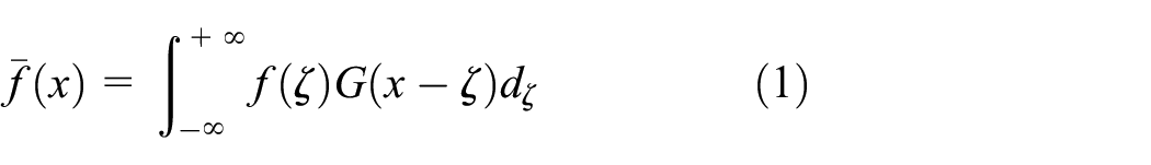
The over bar in the equation represents the filtered quantity. The function f is decomposed into a resolved-scale component $\bar{f} (x)$ and a sub-grid-scale component $f' (x)$ :

f (x) = \bar{f} (x) + f' (x)

(2)

In equation (1), the function $G$ is the filter function. The box filter is the most popular one, and can be expressed as

G (ζ) = {\begin{matrix} \frac{1}{Δ}, if | ζ | < \frac{Δ}{2} \\ 0, otherwise \end{matrix}

(3)

Δ implies the characteristic length scale of the isotropic grid cells, that is, $Δ = {(Δ x_{1} Δ x_{2} Δ x_{3})}^{1 / 3}$ . Δx₁, Δx₂, and Δx₃ are the lengths of the elements in the x, y, and z directions. Substituting equation (2) and applying the filter operation to the NS equations for the flow of an incompressible, viscous, and Newtonian fluid,²⁶ we obtain

\frac{\partial {\bar{u}}_{i}}{\partial x_{i}} = 0

(4)

\frac{\partial {\bar{u}}_{i}}{\partial t} + \frac{\partial}{\partial x_{j}} ({\bar{u}}_{i} {\bar{u}}_{j}) = - \frac{1}{ρ} \frac{\partial \bar{p}}{\partial x_{i}} - \frac{\partial τ_{ij}}{\partial x_{j}} + 2 ν \frac{\partial}{\partial x_{j}} {\bar{S}}_{ij}

(5a)

{\bar{S}}_{ij} = \frac{1}{2} (\frac{\partial {\bar{u}}_{i}}{\partial x_{j}} + \frac{\partial {\bar{u}}_{j}}{\partial x_{i}})

(5b)

where ρ is the fluid density. u_i is the fluid velocity. The subscripts i and j are used here. i or j = 1 represents the x-direction, i or j = 2 represents the y-direction and i or j = 3 represent the z-direction. p is the pressure. $ν$ is the turbulent viscosity, ${\bar{S}}_{ij}$ is the rate of the strain tensor for the resolved large scales, and $τ_{ij}$ is a sub-grid-scale stress tensor:

τ_{ij} = \bar{u_{i} u_{j}} - \bar{u_{i}} \bar{u_{j}}

(6)

$\bar{u_{i} u_{j}}$ is unknown, and needs to be modeled. The Boussinesq hypothesis is employed to calculate the Smagorinsky sub-grid-scale (SGS) stress²⁸:

τ_{ij} = \frac{1}{3} τ_{kk} δ_{ij} - 2 ν_{t} {\bar{S}}_{ij}

(7)

$ν_{t}$ (=μ_t/ρ) is the sub-grid-scale turbulent viscosity.

The wall-adapting local eddy-viscosity (WALE) SGS model was employed to model sub-grid scale turbulence.²⁵ Compared with the Smagorinsky SGS model, the WALE model has the advantage that it considers the effects of turbulent flow near the wall as well as the transfer of momentum. In the WALE model, the viscosity of the sub-grid vortex is zero in the region of pure shear flow. This ensures the accuracy of the modeled numerical flow field within near-wall laminar flow. Moreover, this model is nearly insensitive to the grid resolution for predicting flow separation and swirls.²⁹ In the WALE model, the sub-grid scale turbulent viscosity is described as

ν_{t} = {(C_{w} Δ)}^{2} \frac{{(S_{ij}^{d} S_{ij}^{d})}^{3 / 2}}{{({\bar{S}}_{ij} {\bar{S}}_{ij})}^{5 / 2} + {(S_{ij}^{d} S_{ij}^{d})}^{5 / 4}}

(8)

C_w is a constant, set to 0.325 by default. $S_{ij}^{d}$ is described as ²⁵:

S_{ij}^{d} = \frac{1}{2} ({\bar{g}}_{ij}^{2} + {\bar{g}}_{ji}^{2}) - \frac{1}{3} δ_{ij} {\bar{g}}_{kk}^{2}

(9)

where $δ_{ij}$ is the Kronecker symbol.

{\bar{g}}_{ij} = \frac{\partial \bar{u_{i}}}{\partial x_{j}}

(10a)

{\bar{g}}_{ij}^{2} = {\bar{g}}_{ik} {\bar{g}}_{kj}

(10b)

Computational domain and numerical schemes

The O-shaped computational domain is used to generate an orthogonal mesh by adapting the circular shape of the cylinder as shown in Figure 6. The cylinder is in the center of the domain, and has a radius of 20 D, where D is its diameter. In the literature, the range of the aspect ratio considered between the span length of the cylinder and D varied from zero (2D case) to 2π.²⁴ The span-wise length used here was πD, as in Parnaudeau et al.³⁰ The dimensions and boundary conditions applied to the domain are shown in Figure 6(a). In the flow direction, the front semi-circular surface of the cylinder of the domain was the inlet and the remaining half was the outlet. The free-stream condition was applied to the inlet and the outlet, and cyclic boundary conditions were applied to the top and bottom of the domain. The no-slip boundary condition was imposed on the wall of the cylinder.

Figure 6.

Computational domain and applied boundary conditions (a), and zoomed-in mesh near the surface of the cylinder (b).

As introduced in the previous section, an LES using the WALE SGS turbulence model was employed to predict flow over a circular cylinder at a Re of 1.4 × 10⁵. The open-source computational fluid dynamics (CFD) tool OpenFOAM seven was used as a solver.³² The second-order accuracy PIMPLE algorithm was used to deal with pressure–velocity coupling. It is a combination of Pressure Implicit with Splitting of Operator (PISO) and Semi-Implicit Method for Pressure-linked Equations (SIMPLE). The second-order implicit Euler method was used for time discretization.

Mesh verification

The numerical methods have been employed to approximate the flow separation and turbulent eddies over the spiral grooved cylinder. The results have been validated by benchmarking with the experimental results, as discussed in Chao et al.³⁹ For mesh independence studies, case four was selected for the analysis. Two different meshes N_θ × N_r × N_z were generated, that is, coarse mesh has 414 × 238 × 63 cells and fine mesh has 540 × 300 × 80 cells. N_θ is the number of mesh elements in the θ direction; N_r is the number of mesh elements in the r direction; N_z is the number of mesh elements in the spanwise direction. A very fine mesh was created and attached to the cylinder wall to resolve the viscous sublayer within the flow boundary layer. The first layer of the grid was 3 × 10⁻⁴ D thick and its growth ratio was low, 1.025, in order to capture the steep gradient and discontinuities of the flow. The mesh around the cylinder is shown in Figure 6(b). The time step Δt was adjustable for all cases in temporal iterations to secure y⁺ < 1 based on the criterion that the maximum CFL (Courant number) <0.5. Figure 7 shows the drag coefficients C_D obtained over the non-dimensionlized time T (=tU/D) at Re = 1.4 × 10⁵. It exhibits similar fluctuations as the smooth and rough circular cylinders considered.^40,41,45 There is only a 2% difference in averaged C_D values between two meshes. The fluctuation in C_D is caused by the unstable turbulence in the wake field. In the application of the overhead high-power conductors, the drag exerted on the wire by the strong wind is more concerning than the lift. The mesh resolution of coarse mesh is therefore fine enough to understand the physical insight of the high Re flow. The fine mesh, however, will be used to carry out the rest of the simulations at the different wind speeds to explore the flow behavior in details particularly in the region of flow separation over a wide range of Re. In addition, the mesh is much finer in the cross-sectional plane than the one used in the Cheng et al.²²

Figure 7.

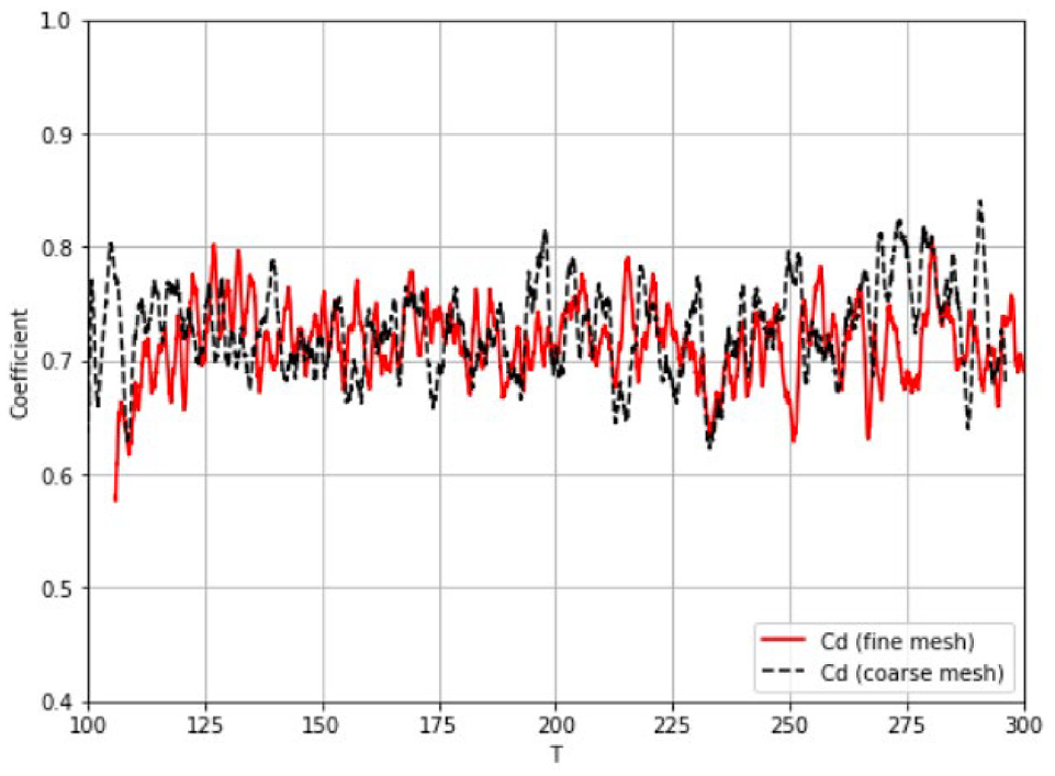
Numerical results of grid independence study based on the coarse mesh and the fine mesh.

Experimental results and discussion

Incoming flow encountered the circular cylinder and clung to its surface before the separation point as shown in Figure 8. The vortices were detached after this point and turbulent flow formed downstream. The flow slowed down in the wake, and a region of much lower pressure was formed. Drag arose due to the difference of the pressure distribution on the windward and leeward surfaces of the cylinder. A number of uncertainties could have influenced the measured values of drag coefficient C_D, such as the level of incoming flow turbulence,³⁷ blockage, and the aspect ratio of the cylinder.¹³ All of these could have yielded different ranges of flow of the critical Re, where the separation angle measured from the front stagnation point changed from about 80° to 100°.¹⁷

Figure 8.

Schematic view of flow separation around a circular cylinder. α = 0° is the most windward point of the cylinder surface and measured in the clockwise direction.

The experimental results of the spiral grooved cylinder exhibited a similar trend on the curve of C_D as a function of Re as was noted by Eguchi et al.² In addition, they fell in the same critical flow region of Re. The performance of the cylinder in case two nearly matched Eguchi et al.’s results as shown in Figure 9. The similarity of the trends of the curves of C_D between their results and ours can be attributed to the similar spiral grooved surfaces of the circular cylinders used. Twelve engraved semi-circular grooves were used in their experiment, as shown in Figure 1(c) and (d).

Figure 9.

Comparison of experimental results of the drag coefficient between the cylinders with semi-circular grooves developed by Eguchi et al.² and the cylinders used in the present study.

The parameter h had a significant effect on the drag coefficient C_D. In the typhoon condition, when Re > 9.3 × 10⁴, the decrease in h led to a lower C_D at both groove angles θ = 15° and 20°. The surface roughness was responsible for this characteristic. The grooves on the surface of the cylinder enlarged the surface area exposed to the flow. This led to an increase in the skin friction and, thus, lower local velocity near the surface. For a lower h, the flow stream clung to the curved surface and delayed the flow separation to the leeward side of the cylinder. However, the disturbance of the grooves at higher values of h led to the formation of the vortices trapped within them. The free shear layer over the opening of the groove was oscillatory.² The shed fluctuation flow grew into large vortices and joined the turbulence wake. This disturbance might have caused the separation point to shift slightly upstream. Thus, the region of turbulence wake was slightly enlarged, which led to a higher C_D. As mentioned above, the use of spiral grooves on the surface of the cylinder to reduce C_D acted like dimples fabricated on a golf ball. The conclusion regarding the effect of h on C_D showed good agreement with that in the study by Aoki et al.⁴ That is, the shallower dimples exerted a lower wind drag.

The different angles θ indicate the different numbers of spiral grooves distributed on the surface of the cylinder in the circumferential direction. The lower θ is, the rougher the surface of the cylinder is. In typhoon conditions, the cylinder with the lower roughness exhibited a lower C_D as shown in Figure 9 by comparing cases 2 and 4, and cases 3 and 5. However, it lost these advantages at lower wind speeds. A significant increase in C_D was noted, especially for case four when Re < 9.3 × 10⁴. To explore the underlying behavior of the fluid, a CFD analysis of this case was considered in the next section.

The experimental results of the spiral grooved cylinder for the mean drag coefficient against Re are shown in Figure 10. The C_D curve of a smooth cylinder was used to estimate the shifting of critical Re, and deviation was observed. This was consistent with the findings by Alonzo-García et al.¹¹ That is, the increase in the surface roughness caused the critical Re to decrease. Figure 10 shows that the critical Re region shifted to the left for all spiral grooved cylinders compared with the smooth cylinder. The drag coefficient was sensitive to Re and decreased only in the flow region of the critical Re. This observation was consistent with the results of wind tunnel tests.¹³

Figure 10.

Comparison of experimental results of the drag coefficient between the smooth cylinder reported by Tritton³⁸ and the spiral grooved cylinders used in this study.

Numerical results and discussion

Drag and lift coefficients

The numerical results of case four at the different wind speeds are presented in Figure 11. The position of the boundary layer separation from the surface of the cylinder affects the frequency of vortex shedding and stabilization of the C_D.⁴¹ The different positions of flow separation determined the behaviors of the shear layers. The roughness of the surface of the cylinder triggered small-scale fluctuations in the separation layer. In Figure 11(a), the transition from the critical to the supercritical flow region of the Re = 1.1 × 10⁵ generated the smallest fluctuation in magnitude of C_D. The same positions of flow separation between the upper and lower surfaces stabilized the pattern of wake flow and reduced the fluctuations in the C_D.⁴² The fluctuation reflected vortex shedding in the wake. It was much regular at Re = 1.1 × 10⁵ compared with the other properties of the flow which performed noisy time series of the force. The coincidence of flow separation on the surface of the cylinder and the alternate vortex shedding in the wake might have caused this. The oscillation of the C_L values was owing to the alternately vortex shedding from the two lateral sides of the cylinder.⁷ The amplitude of fluctuation of the lift was greater than that of the drag. It was hard to find the dominant frequency for Re = 9.3 × 10⁴ and 1.4 × 10⁵. On the contrary, for other cases, flow separated from the surface of the cylinder suppressed the vortex in the wake, resulting in regular variations in C_L magnitude.

Figure 11.

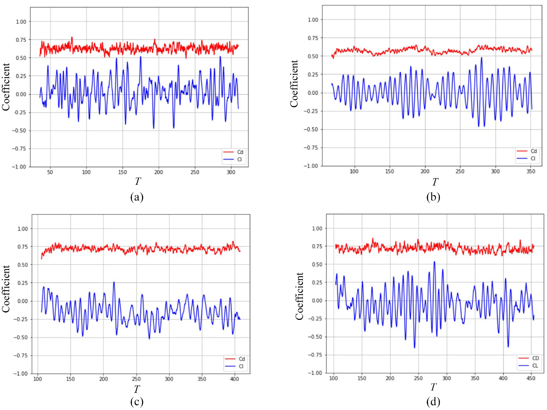
Time histories of C_D and C_L at different speeds of the incoming flow: (a) Re = 9.3 × 10⁴; (b) Re = 1.1 × 10⁵; (c) Re = 1.4 × 10⁵; and (d) Re = 1.6 × 10⁵.

The features of wake flow were represented by the Strouhal number St, which is expressed as fD/U, where f is the frequency of vortex shedding. Figure 12 illustrates the FFT (fast Fourier transformation)-based spectral analysis of C_L. Each part shows a unique characteristic with varying incoming flow velocities. A broad spectral content with more than one large amplitude was observed in the flow region of the critical Re = 9.3 × 10⁴. It reflects the unstable flow state due to the presence of the low-frequency spectrum. This can be attributed to the mixture of other typical vortices of the oscillations of the wake, because of which the shedding frequency became ambiguous. The same phenomenon was presented by Kiani and Javadi on a flagged short-finite circular cylinder.⁴³ This flow behavior can also be found in the region of super flow at critical values of Re from 5 × 10⁵ to 3.5 × 10⁶ for a smooth circular cylinder.⁴⁴ As the velocity increased, the dominant frequency of vortex shedding was as shown in Figure 12(b) and (d). The flow fell in the transitional state from critical to supercritical Re flow. The amplitudes increased. Only Figure 12(b) presents a narrowband spectrum with S_t = 0.13. The high frequencies of the St values at the peak amplitudes as a function of Re are plotted in Figure 13(a). The St value at Re = 9.3 × 10⁴ was more than 0.2, similar to that of the smooth circular cylinder at a subcritical Re.¹⁵ The decrease in values of St was evident as wind speed increased. The average values of the C_D were compared with the experimental results as shown in Figure 13(b). They matched each other well. The maximum difference is 11% at Re = 1.4 × 10⁵.

Figure 12.

FFT spectra of the lift coefficient C_L at different speeds of incoming flow: (a) Re = 9.3 × 10⁴; (b) Re = 1.1 × 10⁵; (c) Re = 1.4 × 10⁵; and (d) Re = 1.6 × 10⁵.

Figure 13.

(a) Strouhal number St against the Re and (b) comparison between experimental and numerical results for case 4.

Flow separation from the surface of the cylinder

The presence of the grooves enhances the roughness of the cylinder surface. It causes the complexity of the flow characteristics. To explore flow separation because of the influence of the spiral grooves, the streamlines of the mean velocity in the middle cross-sectional plane of the cylinder are plotted for different Re in Figure 14. The letters in figure indicate different flow behaviors inside each groove. “N” stands for attached flow, “C” for the trapped separation bubble in the clockwise direction, “P” for the position of the primary recirculation zone of the mean flow which is denoted with dashed red line, and “A” for the trapped separation bubble in the anti-clockwise direction. At Re = 9.3 × 10⁴ as shown in Figure 14(a), one “C” was noted at x = 0 before the primary recirculation zone “P.”²² The groove-sized “P” owing to the higher shear stress near the wall, followed by a clock-wise second bubble “C.” On the contrary, “P” was followed by the anti-clockwise trapped bubbles for Re = 1.1 × 10⁵, 1.4 × 10⁵, and 1.6 × 10⁵ which was similar to the observation of LES results.²² When Re = 1.1 × 10⁵ as shown in Figure 14(b), the primary recirculation zone “P” moved slightly upstream, followed by an anti-clockwise flow bubble within the same groove. Further downstream, a groove-scale anti-clockwise flow bubble was formed. The primary recirculation zones and their upstream clockwise bubbles became larger as Re was increased from Re = 1.1 × 10⁵ to Re = 1.6 × 10⁵. Furthermore, they had similar flow bubbles except that the anti-clockwise flow bubble became very small when Re = 1.6 × 10⁵, as shown in Figure 14(d). In a nutshell, the grooves caused the recirculation flow and the separation bubbles to form within them.^45,46 Due to their presence, flow separation from the cylinder surfaces is delayed, resulting in much narrower wake fields than those observed in the same range of Re for a smooth cylinder (see Figure 14(e)).⁴⁷ This resulted in a decrease in C_D. It is consistent with the Wan Yahaya et al.⁴⁸ Thus, the grooved cylinders have much lower C_D values as depicted in Figure 10.

Figure 14.

Streamlines of mean velocity in the middle plane of the grooved cylinder: (a) Re = 9.3 × 10⁴; (b) Re = 1.1 × 10⁵; (c) Re = 1.4 × 10⁵; (d) Re = 1.6 × 10⁵; and (e) streamlines for the smooth cylinder at Re = 1.0 × 10⁵.⁴⁷

Q-criterion field

Iso-surfaces of the Q-criterion⁴⁹ colored by u_x are plotted in Figure 15 to visualize the structure of instantaneous flow at different incoming flow speeds. The instantaneous iso-surfaces are Q = 5 × 10⁵. The figures in the left column show the zoomed-in view of the flow structure near the surface of the cylinder. The flow separated from the spiral grooved surface was noted, and joined the turbulence downstream. Along the span-wise direction, for all cases, the turbulent flow shed from the cylinder is observed parallel to the central axis of the cylinder. As the velocity increased, flow along each spiral quickly broke into small scales and irregularly shed from the surface of the cylinder. In Figure 15, the plots in the right column show the wake flow. The wake field became longer with increasing incoming velocity. In addition, the scale of the flow structure grew very large at higher velocities. At Re = 1.1 × 10⁵, alternate vortex shedding was observed along the wake but not in the other cases. This might have caused the regular fluctuation in the curve of lift coefficient in Figure 11(b). The disappearance of vortex shedding reduced fluctuation in the aerodynamics of the cylinder and further diminished the chance of fatigue in the conductor wire in the practical application. Unlike for the straight grooved cylinder, vortex shedding was more apparent in this case.²²

Figure 15.

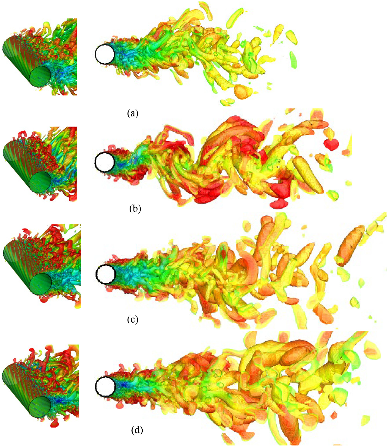
Structures of instantaneous flow near the surface of the cylinder and downstream flow when iso-surfaces of Q-criterion are at Q = 5 × 10⁵ colored by u_x: (a) Re = 9.3 × 10⁴; (b) Re = 1.1 × 10⁵; (c) Re = 1.4 × 10⁵; and (d) Re = 1.6 × 10⁵.

Pressure and skin-friction coefficients

The pressure distribution on the cylinder surface responds to the dominant part of the total drag. Figure 16 shows the pressure coefficient C_p for case four against the azimuthal angle α with different Re. A sketch of the projected groove profile alone the angle α is also shown in Figure 16 to localize the corresponding changes in pressure. Due to grooves on the surface of the cylinder, C_p showed a local rebound at each groove before reaching the minimum value at approximately α = 60° which is lower than the result at Re = 3900, the cylinder with straight grooves.²² After that, the C_p increased, then decreased, and finally rebounded back to become a flattened plateau. There is one groove between 60° and 90°. So the pressure increased due to the slowdown of the velocity within the groove. As shown in Figure 14, at 90°, the clock-wise separation bubble was formed within the groove, which caused the lower pressure compared to the smoothed surface cylinder.²² The plateau trend started around 120°. Comparing it to the smoothed surface cylinder, whose plateau region of C_p curve started at about 90° in the Cheng et al.,⁴⁷ it shifted backward. This implied that the flow separation points on the surface move further back in the cylinder leeward side. This caused a narrower low pressure wake. As a result, the drag on the cylinder was reduced.

Figure 16.

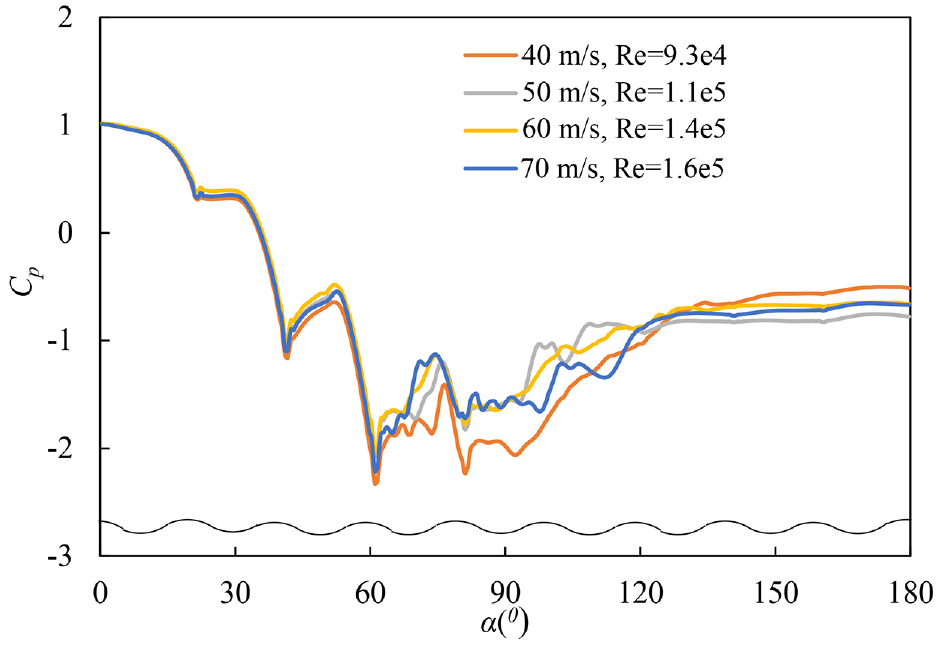
Pressure coefficient C_p over the grooved cylinder surface with different Re.

The skin-friction coefficient C_fθ over the grooved cylinder surface is presented in Figure 17. It is the ratio between the wall shear stress and the local dynamic pressure within flows along the boundary layer (= $τ / 0.5 ρ U^{2},$ $τ$ is the shear stress). With grooves, its rapid variation that occurred when α < 80° was similar to that of a circular cylinder with 12 columns of dimples on its surface.⁶ The maximum values C_fθ was at about α = 60° independent of Re, the wall shear stress was greatest whereas the pressure was the lowest as depicted in Figure 16. But for the surface smoothed cylinder, the maximum C_fθ was at about α = 50°.^6,22 As shown in Figure 17, the presence of the grooves caused C_fθ to decrease for the location of α < 80°. As a results, the skin friction drag was lower than that of the surface smoothed cylinder, since the skin friction drag is obtained by integrating. The same conclusion was also drawn from the dimpled circular cylinders.⁶ The peak C_fθ values decreased as Re increased at each bulge position of the cylinder for α < 80°. C_fθ values tended to be less fluctuation and closed to zero for α > 80°, after flow separation occurred. On the leeward surface of the cylinder, the separated bubbles were trapped within grooves, and led to a lower C_fθ. The higher C_fθ values before flow separation indicated that the surface shear stress on the windward surface dominated the overall value of C_fθ.

Figure 17.

Skin-friction coefficient C_fθ over the grooved cylinder surface with different Re.

Figure 18 shows the instantaneous surface skin-friction lines. 0° indicated on the cylinder surface is the stagnation point as presented in Figure 8. Figure 18(a) to (d) illustrate the windward walls of the cylinders at the different wind speeds. There is no significant difference in the lines pattern. At 0°, the stagnation points formed a vertical straight line in the spanwise direction. The horizontal straight skin-friction lines were visible at both sides of the stagnation points. Surface-smoothed cylinders exhibited the same flow patterns as the Cheng et al.²² The trajectories of skin-friction lines changed directions and followed the grooves pattern at about α = 30° and 330°. Disturbance of the grooves were probably responsible for this. The patterns of skin-friction lines on the windward side of the cylinder indicated the wall-attached boundary-layer flow. Chaotic flow separation began at about α = 80° as shown in Figure 18(e) to (h). This angle was approximately 72° for a surface-smoothed cylinder with Re = 10⁵. Therefore, grooves could reduce the turbulent flow region, thereby reducing the wind drag. The skin-friction coefficient was quite low after this angle, as shown in Figure 17.

Figure 18.

Skin-friction lines on the cylinder surfaces: (a–d) are windward views, (e–h) are side views. The incoming flow direction is depicted in Figure 8. Re = 9.3 × 10⁴ for (a, e), Re = 1.1 × 10⁵ for (b, f), Re = 1.4 × 10⁵ for (c, g), and Re = 1.6 × 10⁵ (d, h).

The top row of Figure 19 displays the vortex lines on the cylinders’ windward sides. The line patterns followed the grooves and were remarkably similar, no matter what the wind speed was. Similar to the skin-friction lines, the patterns were disrupted at approximately 80°. The critical transition points from the wall-attached flow to the vortex flow were difficult to identify, but the separation was obvious in the surface-smoothed cylinder at Re = 10⁵.²²

Figure 19.

Surface vortex lines on the cylinder surfaces: (a–d) are windward views, (e–h) are side views. The incoming flow direction is depicted in Figure 8. Re = 9.3 × 10⁴ for (a, e), Re = 1.1 × 10⁵ for (b, f), Re = 1.4 × 10⁵ for (c, g), and Re = 1.6 ×10⁵ (d, h).

Conclusions

Experimental and numerical studies have been conducted on the spiral grooved cylinder in the typhoon conditions. The findings are as follows.

The experimental results have shown that a decrease in groove depth h leads to a lower C_D at both groove angles θ = 15° and 20° when Re > 9.3 × 10⁴.

More spirals on the surface of the cylinder maybe detrimental to drag reduction in the typhoon conditions. A rougher surface of a cylinder increases the surface area exposed, reduces the local velocity, and increases skin resistance.

The critical Re decreases when the spiral grooves are applied to the surface compared with a smooth circular cylinder.

A lower drag coefficient has been obtained in the typhoon conditions, but the roughness exerted high wind drag in low-wind conditions when Re < 9.3 × 10⁴.The numerical results have shown a good agreement with the experimental results and the maximum difference is about 11%.

A larger fluctuation of the drag coefficient has been noted in the flow region of the critical Re, whereas the smallest fluctuation occurred in the region of transitional Re = 1.1 × 10⁵.

The mixture of typical vortices of the wake oscillations and the shedding frequency have led to higher magnitudes of fluctuation. As a result, the fluctuation has caused a much higher C_L than in C_D.

It has been observed that small-scale eddies shed from the spiral grooves and become the very large flow structures further downstream.

The increase in Re led to the longer wake and the lower surface shear stress on the windward surface of the cylinder.

Although this study provides a basis for future work in the area, the underlying physics of flow in flow regions of different Re values remains unclear. Furthermore, in the numerical analysis, the length of the cylinder may have a non-negligible impact on the features of the flow along the span-wise direction, and could help capture fluid behavior as seen in the wind tunnel. Further investigation is needed to consider cylinders with longer length in future research.

Footnotes

Appendix

Handling Editor: Chenhui Liang

Declaration of conflicting interests

The author(s) declared no potential conflicts of interest with respect to the research, authorship, and/or publication of this article.

Funding

The author(s) received no financial support for the research, authorship, and/or publication of this article.

ORCID iD

Jing Liu

References

Sakakibara

Iisaka

Mori

, et al. Development of low-wind-pressure conductors for compact overhead transmission line. IEEE Trans Power Apparatus Syst 1984; PAS-103: 3117–3124.

Eguchi

Kikuchi

Kawabata

, et al. Drag reduction mechanism and aerodynamic characteristics of a newly developed overhead electric wire. J Wind Eng Ind Aerodynamics 2002; 90: 293–304.

Hiratsuka

Matsuzaki

Fukuda

, et al. Field test results of a low wind-pressure conductor. In: Proceedings of IEEE region 10 international conference on electrical and electronic technology, TENCON 2001 (Cat. No. 01CH37239), August 2001, vol. 2, pp.664–668. New York: IEEE.

Aoki

Ohike

Yamaguchi

, et al. Flying characteristics and flow pattern of a sphere with dimples. J Visual 2003; 6: 67–76.

Zhou

Wang

Guo

, et al. Experimental study on flow past a circular cylinder with rough surface. Ocean Eng 2015; 109: 7–13.

Yan

Yang

Wang

Study of the drag reduction characteristics of circular cylinder with dimpled surface. Water 2021; 13: 197.

Canpolat

Sahin

Influence of single rectangular groove on the flow past a circular cylinder. Int J Heat Fluid Flow 2017; 64: 79–88.

Afroz

Sharif

MAR

. Numerical study of cross-flow around a circular cylinder with differently shaped span-wise surface grooves at low Reynolds number. Eur J Mech B/Fluids 2022; 91: 203–218.

Saito

Hasc

Eguchi

, et al. Spiral-elliptic conductor with low-drag coefficient [for overhead power lines. In: 2000 IEEE power engineering society winter meeting. conference proceedings (Cat. No. 00CH37077), January 2000, vol. 4, pp.2397–2402. New York: IEEE.

10.

Matsumura

Yura

Kikuchi

, et al. Development of low wind-pressure insulated wires. Furukawa Electr Rev 2002; 39–44.

11.

Alonzo-García

Gutiérrez-Torres

CDC

Jiménez-Bernal

JA.

Large eddy simulation of the subcritical flow over a U-grooved circular cylinder. Adv Mech Eng 2014; 6: 418398.

12.

Liu

Wang

Zhu

, et al. The influence of the opening angle of conductor surface on the drag coefficient. In: 2017 7th international conference on advanced design and manufacturing engineering (ICADME 2017), July 2017, pp.440–445. Atlantis Press.

13.

Ahmed

Haque

Rauf

MA.

Investigation of drag coefficient at subcritical and critical Reynolds number region for circular cylinder with helical grooves. Int J Marit Technol 2017; 8: 25–33.

14.

Farell

Blessmann

On critical flow around smooth circular cylinders. J Fluid Mech 1983; 136: 375–391.

15.

Yeon

Yang

Stern

Large-eddy simulation of the flow past a circular cylinder at sub- to super-critical Reynolds numbers. Appl Ocean Res 2016; 59: 663–675.

16.

Kim

Mohan

. Prediction of unsteady loading on a circular cylinder in high Reynolds number flows using large eddy simulation. In: International conference on offshore mechanics and arctic engineering, January 2005, vol. 41979, pp.775–783.

17.

Talley

Mungal

. Flow around cactus-shaped cylinders. Stanford, CA: Center for Turbulence Research Annual Research Briefs, 2002, p.363.

18.

Ladjedel

Yahiaoui

Adjlout

, et al. Experimental and numerical studies of drag reduction on a circular cylinder. World Acad Sci Eng Technol 2011; 77: 357–361.

19.

Travin

Shur

Strelets

, et al. Detached-eddy simulations past a circular cylinder. Flow Turbul Combust 2000; 63: 293–313.

20.

Wang

Liu

Zhang

QS.

Measurement of flow around a cactus-analogue grooved cylinder at red=5.4×10⁴: wall-pressure fluctuations and flow pattern. J Fluids Struct 2014; 50: 120–136.

21.

Catalano

Wang

Iaccarino

, et al. Numerical simulation of the flow around a circular cylinder at high Reynolds numbers. Int J Heat Fluid Flow 2003; 24: 463–469.

22.

Cheng

Pullin

Samtaney

Large-eddy simulation of flow over a grooved cylinder up to transcritical Reynolds numbers. J Fluid Mech 2018; 835: 327–362.

23.

Zhao

Duan

, et al. Numerical analysis of hydroenergy harvesting from vortex-induced vibrations of a cylinder with groove structures. Ocean Eng 2020; 218: 108219.

24.

Pereira

Vaz

Eça

. Flow past a circular cylinder: a comparison between RANS and hybrid turbulence models for a low Reynolds number. In: International conference on offshore mechanics and arctic engineering, May 2015, vol. 56482, p.V002T08A006. American Society of Mechanical Engineers.

25.

Nicoud

Ducros

Subgrid-scale stress modelling based on the square of the velocity gradient tensor. Flow Turbul Combust 1999; 62: 183–200.

26.

Nichols

RH.

Turbulence models and their application to complex flows, revision 4.01. University of Alabama at Birmingham (HPCMP/PET CFD Onsite–AEDC), 2009.

27.

Leonard

Energy cascade in large-eddy simulations of turbulent fluid flows. In: Dmowska

(ed.) Advances in geophysics. Amsterdam: Elsevier, 1975, vol. 18, pp.237–248.

28.

Smagorinsky

. General circulation experiments with the primitive equations: I. The basic experiment. Mon Weather Rev 1963; 91: 99–164.

29.

Arya

Effect of grid sensitivity on the performance of wall adapting SGS models for LES of swirling and separating–reattaching flows. Comput Math Appl 2019; 78: 2035–2051.

30.

Parnaudeau

Carlier

Heitz

, et al. Experimental and numerical studies of the flow over a circular cylinder at Reynolds number 3900. Phys Fluids 2008; 20: 085101.

31.

West

Apelt

CJ.

The effects of tunnel blockage and aspect ratio on the mean flow past a circular cylinder with Reynolds numbers between 10 4 and 10 5. J Fluid Mech 1982; 114: 361–377.

32.

Greenshields

CJ.

OpenFOAM user guide. version 6. New Castle, DE: Open FOAM Foundation Ltd, 2017.

33.

Wang

Zhang

, et al. 2016. Structure design and service performance study of low wind-pressure conductor. In: MATEC web of conferences, vol. 44, p.01094. EDP Sciences.

34.

Nader

dos Santos

Jabardo

, et al. Characterization of low turbulence wind tunnel. In: XVIII IMEKO world congress-metrology for a sustainable development, 2006.

35.

Manshadi

. The importance of turbulence in assessment of wind tunnel flow quality. In: Lerner

Boldes

(Eds.) Wind tunnels and experimental fluid dynamics research, 2011, pp.261–278.

36.

Cantwell

Coles

An experimental study of entrainment and transport in the turbulent near wake of a circular cylinder. J Fluid Mech 1983; 136: 321–374.

37.

Stroman

JC.

Aerodynamic drag coefficients of a variety of electrical conductors. Doctoral Dissertation, Texas Tech University, 1997.

38.

Tritton

DJ.

Physical fluid mechanics. 2nd ed. Oxford: Clarendon Press, 1988, pp.21–34.

39.

Chao

Jun

Mingnian

, et al. Large eddy simulation of flow over a new type of low-wind-pressure conductor using WALE model. In: 2019 16th international Bhurban conference on applied sciences and technology (IBCAST), January 2019, pp.811–815. New York: IEEE.

40.

Chen

XY.

Large-eddy and detached-eddy simulations of the separated flow around a circular cylinder. J Hydrodyn 2007; 19: 559–563.

41.

Rodriguez

Lehmkuhl

Piomelli

, et al. LES-based study of the roughness effects on the wake of a circular cylinder from subcritical to transcritical Reynolds numbers. Flow Turbul Combust 2017; 99: 729–763.

42.

Rodríguez

Lehmkuhl

Chiva

, et al. On the flow past a circular cylinder from critical to super-critical Reynolds numbers: wake topology and vortex shedding. Int J Heat Fluid Flow 2015; 55: 91–103.

43.

Kiani

Javadi

Investigation of turbulent flow past a flagged short finite circular cylinder. J Turbulence 2016; 17: 400–419.

44.

Halse

KH.

1997. On vortex shedding and prediction of vortex-induced vibrations of circular cylinders.

45.

Jie

Liu

YZ.

Large eddy simulation of turbulent flow over a cactus-analogue grooved cylinder. J Visual 2016; 19: 61–78.

46.

Zheng

Zhou

Zhong

, et al. An experimental investigation of drag and noise reduction from a circular cylinder using longitudinal grooves. Phys Fluids 2021; 33: 115–110.

47.

Cheng

Pullin

Samtaney

, et al. Large-eddy simulation of flow over a cylinder with from 3.9×10³ to 8.5×10⁵: a skin-friction perspective. J Fluid Mechanics 2017; 820: 121–158.

48.

Wan Yahaya

WMA

Samion

Mohd Zawawi

, et al. The evaluation of drag and lift force of groove cylinder in wind tunnel. J Adv Res Fluid Mech Therm Sci 2020; 68: 41–50.

49.

Haller

An objective definition of a vortex. J Fluid Mech 2005; 525: 1–26.

Experimental and numerical investigation of flow over spiral grooved cylinders

Abstract

Keywords

Introduction

Experimental setup

Numerical methods for flow simulation

Turbulence model

Computational domain and numerical schemes

Mesh verification

Experimental results and discussion

Numerical results and discussion

Drag and lift coefficients

Flow separation from the surface of the cylinder

Q-criterion field

Pressure and skin-friction coefficients

Conclusions

Footnotes

Appendix

Declaration of conflicting interests

Funding

ORCID iD

References