Sage Journals: Discover world-class research

Abstract

The driving safety of heavy-haul train is affected by the train’s traction weight, the length of train, the line profile, the line speed limit, and other factors. Generally, when the train is running on a continuously long and steep downgrade line, it needs using the circulating air braking to adjust speed. When it is braking, the brake wave is transmitted non-linearly along the direction of the train. When it is relieved, it must be ensured that there is sufficient time for the train to be inflated. Therefore, it is difficult to ensure the safe operation of the heavy-haul train. In this article, a new method of the train’s driving strategy based on improved genetic algorithm is proposed. First, a mathematical model for the operation of heavy-haul train is established with multiple parameters. Then, according to the improved genetic algorithm and the mathematical model of the heavy-haul train, the driving strategy of the chromosome of the train is studied. Finally, the driving curve which can ensure the safe running of the heavy-haul train can be obtained. By comparing the simulated driving curve with the actual one, the results show the effectiveness of the proposed method.

Keywords

Heavy-haul train improved genetic algorithm driving strategy simulation modeling multi-particle model

Introduction

During the driving process of the heavy-haul train, the train will be subjected to the joint force in the transverse, longitudinal, and vertical directions in the course of operation, and the force condition is more complicated.¹ Lateral dynamics mainly affects the stability of train’s operation. The force in the vertical direction is mainly the support force of the train. The safe operation control focuses on the relationship between the force and the acceleration during the train’s operation, so the longitudinal stress of the train along the track direction is mainly considered. The safe operations of heavy-haul trains are subjected to many restrictions in practical applications, and their performances are related to many complex factors, such as traction force, train’s length, speed limitations, and continuous long and steep downgrade grades. In particular, when the train is running in the section that the line grades change frequently, the train’s braking or traction always makes the longitudinal impulsive force of the train intensified, and the longitudinal force of each vehicle is increased. For heavy-haul trains with air braking, the vibrated longitudinal force can cause more severe damages. In specific, the change in longitudinal force brings changes in the longitudinal length of the train, which eventually transforms the train into a complicated vibration system of multi-degree of freedom. In practice, it is a big challenge to ensure the safety of running trains on heavy-haul lines. This article aims to propose a scheme based on the conditions of railway lines (line grade, length, speed limit, etc.) and the situation of the train marshalling (which includes traction weight of trains and the train’s length) to obtain a optimal driving strategy of train to ensure the safety of the running train.

There are many existing studies on the control strategy of rail transit trains. In terms of urban rail transit, the dynamic adjustment of train’s operation process was realized using the fuzzy self-tuning control strategy of differential evolution in Chang and Xu.² Mitsukawa³ carried out an expert system to realize the control of the automatic speed of the rail transit train. An automatic control of train is realized by combining a fuzzy control and predictive control algorithm in Yu and Chen.⁴ But this algorithm had high computation complexity, and it needs to take a large amount of computing resources. Yu et al.⁵ proposed a particle swarm optimization algorithm to achieve multi-objective train control, which, however, is time consuming for practical implementations. Xun et al.⁶ presented a cellular automata to realize the multi-objective optimal control of train’s operation process. But the considered factors in this study are not comprehensive, such as the track of the running of the train and the operation curve. Zhao and Gao⁷ studied a method of automatic operation of urban rail transit trains based on improved predictive control. This approach uses a way to reduce overshoot to optimize multiple targets. And multi-step prediction, online optimization, and feedback correction of the optimization results were also carried out. Hou et al.⁸ discussed an application based on the model-free adaptive control of train control and parking algorithm. This algorithm achieved a good control effect by iterative learning of train’s operation data. Yin et al.⁹ proposed an intelligent train operation algorithm for subway by expert system and reinforcement learning, which can obtain a good result in train’s energy-saving and time-saving for urban rail transit.

In high-speed railways, a parameter identification technology based on the train’s model of train’s operation control system was employed.^10,11 Song and Song¹² adopted an adaptive control technology, which can realize the automatic speed control of the train. Li¹³ studied an optimization strategy of electric multiple unit (EMU) operation and proposed a rolling optimization by the method of evaluation of the advantages of extension theory. Feng¹⁴ presented a linear quadratic regular (LQR) control algorithm into automatic train control (ATO), and many of its performance targets achieved good results. Li¹⁵ proposed an adaptive control algorithm of high-speed train to control the speed. And a Lyapunov function was used to calculate the mass of the train under stochastic variation. During the course of train’s operation, Sandidzadeh and Shamszadeh¹⁶ discussed a kind of fuzzy control rule combining the actual driving experience to improve the control effect.

Nevertheless, it is worth mentioning that the existing control strategies on urban rail trains and high-speed trains are difficult to be applied to the heavy-haul railway due to the following reasons:

The length of the heavy-haul train can be very long and each train can be composed by more than 100 vehicles. And the maximum length of the train is more than 1.5 km.¹⁷ When the train is using the air braking, there is a huge elastic deformation force produced by the changes in internal longitudinal movement. Meanwhile, the whole train, like an elastic mechanical vibration system, has longitudinal tensile and compression. In the operation of urban rail transit and high-speed railway, the train connection is considered to be rigid, indicating that there is no tension and compression change.¹⁸ In the urban rail transit train, there are many power vehicles. The train usually uses a power vehicle to drag a carriage. Therefore, when the train is braking or in traction, its internal longitudinal force change is relatively small and the train’s integrity is good, while heavy-haul trains are single locomotive, pulling hundreds of vehicles. When the train is accelerating or braking, the longitudinal force of the train changes greatly and it is very easy to damage the coupler, causing accidents. Therefore, when calculating the driving strategy of the heavy-haul train, it is particularly needed to consider the effect of train’s longitudinal forces.

The heavy-haul train in the long and steep downhill needs to take the circulating air braking to adjust the speed.¹⁹ And in this process, the transmission of air-braking wave has nonlinear characteristics, which may easily cause fracture of coupler under the condition of improper driving strategy. Since urban rail transit and high-speed railway line have small gradients, the train mainly adopts the dynamic braking to realize the synchronous adjustment of the speed. So, the driving strategy of the heavy-haul train must take into account the safety of trains running on long and steep slopes.

The equivalent virtual braking distance and time are mainly related to the length of the train and the number of vehicles. The number of vehicles in each heavy-haul train is more than that of urban rail trains and high-speed trains, which will inevitably lead to a long braking time and distance of the heavy-haul train. In addition, the pressure gradient of long trains has an effect on the braking force of the rear vehicles. So, when the train is braking, if the braking time and distance cannot be calculated accurately, it is prone to exceed the speed limit and it cannot guarantee that the train has enough air-filled time, which is likely to cause accidents.

Many scholars are studying the driving control technology of heavy-haul trains, and they have made a lot of achievements. Chou et al.²⁰ analyzed the train’s longitudinal impulse of the heavy-haul train equipped with electrically controlled pneumatic (ECP) braking system and designed the LQR closed-loop optimal controller based on full-state feedback. In addition, when we analyze and calculate the longitudinal force of the train in our study, the method we used refers to the method of the cited article. Also, our work is inspired by this article in terms of train’s modeling and the validity description of the result. Khmelnitsky²¹ proposed the decentralized control model to control the speed of a single vehicle. But the complexity of the algorithm is very high. Wong and Ho²² took advantage of crossover and selection mechanism of genetic algorithm and heuristic search to obtain the train’s coast points. But when the input data were large, the algorithm took a long time. Wang and Ma²³ carried out a basic principle and methods of artificial intelligence to the research on the expert system of the control technology of the heavy-haul train. But the subjectivity of expert system was much stronger, and it was difficult to obtain the database. Huang et al.²⁴ proposed a back propagation (BP) neural network algorithm to model the train’s braking operation process. But the method needed a large number of actual driving data for neural network learning. Qin et al.²⁵ studied a fuzzy control strategy to analyze the whole operation process of the heavy-haul train. Kang²⁶ proposed the predictive control theory to estimate the train’s running speed, and a good result was obtained using this method to determine the train’s working condition conversion point. Ke et al.^27,28 presented a max–min ant algorithm based on the fuzzy control algorithm, which studied the train’s operation control strategy under the condition of variable ramp and variable speed. Bing et al.²⁹ explored an ATO control strategy designed by combining fuzzy control with proportional–integral–derivative (PID) control method. The train’s operation model is established by extracting the experimental data, which improves the system response speed and accuracy. Khmelnitsky²¹ considered the specific constraints (such as temporary speed limit, line condition, and running time) and proposed an iterative algorithm to solve the velocity curve. The driving model based on the traction characteristics of speed and displacement is established, which took the kinetic energy as the state variable. Howlett and colleagues^30,31 carried out the maximum principle for optimal operation strategy of train. For different trains and different ramp lines, the mode conversion condition of train’s energy-saving driving is studied. Vu³² proposed a control strategy based on Pontryagin principle to help train stay on time and reduce energy use. Zhang and Zhuan³³ tried to schedule the train during a long period of travel in a model predictive control (MPC) framework and designed an optimal control methodology for heavy-haul trains with the objective to optimize the train’s operation in terms of energy consumption, velocity tracking, and operation safety. Zhuan and Xia³⁴ proposed an approach of output regulation with measurement feedback for the control of heavy-haul trains.

When a new heavy-haul line is opened, it is necessary for experienced drivers to drive the train for many times to obtain the driving curve to ensure the safe driving of the train. There are huge security risks. The method proposed in this article can be used for different train groups and different line information, and automatically generates the driving curve to ensure the safety of trains. First, we establish the running equation of the train by analyzing the force of the train in the running process on the line, and find the train’s operating constraints, such as running time, distance, speed limit, and line gradient. The formulated model is a nonlinear optimization problem with complex constraints. In this article, the constraints of several conditions are transformed into penalty functions and the problem is converted into a nonlinear unconstrained problem. Second, the genetic algorithm is developed, in which the first step is to encode the driving control model of the train. The running state of the train in the interval is mainly decided by the combination order of four kinds of working conditions, that is, traction, inertia, dynamic braking and air braking, and the position of switching. In this article, the train’s running condition and location are used as variables to encode the chromosome. Thus, the sequence of these conditions constitutes the gene of the chromosome. And the operating conditions are calculated according to the constraints of the train’s traction calculation, running time, and air-braking characteristics. Then, we calculate the fitness function from the two aspects of speed and punctuality rate. Finally, in the process of propagation and evolution of genetic algorithm, we use selective replication operator, crossover operator, and mutation operator to get the simulation results and verify the results.

Since the line conditions of the heavy-haul train are complicated, on the one hand, the data of train’s running time, distance, line speed limit, and line gradient are considerable; on the other hand, the constraints on the train control model will also increase. As well, the number of train groups is increasing, which will inevitably lead to the deterioration of the air braking and the multiplied increase in the longitudinal force. In this case, the calculation of traction calculation and air braking can be very complicated. The traditional genetic algorithm always falls into the local optimal solution and causes premature. And it is generally unable to find a global operation strategy to ensure the security, or it is difficult to find the optimal solution to solve the problem in a finite time. Therefore, the improved genetic algorithm is adopted in this article to overcome this issue.

In this article, we propose an improved genetic algorithm. To avoid emergence of premature caused by not finding the global optimal driving strategy, the strategy of multi-populations evolving in parallel is employed. Different populations use the same genetic strategy, and the various populations are not able to interchange information until they meet the conditions. So, the performance of the algorithm can be improved.

In addition, due to the huge amount of data that the train needs to process, an adaptive adjustment strategy of crossover operator and mutation operator parameters is used to ensure that the algorithm can obtain the results in a reasonable time. When the number of outstanding individuals in the population increases, the probability of crossover and mutation operators will become smaller and smaller, so as to ensure the optimal solution in the population proportion increases.

Train’s operation equation and improved genetic algorithm

In this article, an appropriate model to study the train’s operation was established according to the train’s position, speed, and line ramp’s slope and length, speed, and other parameters, combined with the analysis of longitudinal force dynamics along the running direction of the train.

And then, using the natural selection and genetic mechanism of genetic algorithm, the running process of the train is studied by means of adaptive global optimization.³⁵

Train’s operation equation

When the train does not brake, the brake pipe pressure is kept constant which is generally 500 or 600 kPa. But when the train implements air braking, the pressure of the train pipe is reduced to slow down the speed of the train. The train’s decompression is nonlinear. When the train is filled with wind to relieve braking, air braking cannot simultaneously achieve remission of all wagons, because relief wave is transmitted from the front to back by the vehicle. So, it needs time to ensure the braking ability next time. When the train is in the continuous long and steep downgrade sections, the train needs a cycle of air braking. Therefore, it is difficult for the driver to operate. In this article, we study the train’s running in the following situation.

Assume that there are two or more continuous downgrades in front of the running line, and the length of the front downgrade is not less than 2 km. As shown in equation (1)

{\begin{matrix} j_{i} > 0 \cap j_{i + 1} < 0, j_{i + 2} < 0, \dots \\ j_{i} \leq 0 \cap j_{i + 1} < 0, j_{i + 2} < 0, \dots \\ (s_{i + 1} + s_{i + 2} + \dots) \geq 2000 \end{matrix}

(1)

where j(‰) is the gradient, s (m) is the slope length, and i represents the ith downgrade of the line.

In the running direction of the heavy-haul train, the traction force, the braking force, the basic resistance, and the additional resistance are four different types of forces. Among them, the basic resistance includes mechanical resistance and aerodynamic resistance, that is, friction resistance of axle bearings, rolling friction between wheel and rail, sliding friction resistance between wheel and rail, impact resistance, and air resistance.

When calculating the equation of train’s motion, we take a locomotive or vehicle as a unit, simplify it as a particle, and analyze the stress situation of each particle. A particle chain can be formed by connecting a plurality of locomotives or vehicles together. The model can accurately reflect the force of the train at the variable slope point and variable curvature point.

The force analysis is shown in Figure 1.

Figure 1.

Force analysis model of the train.

As shown above, for the analysis of the nth vehicle, we define that N_n is the force that the ground support for the train, G_n is the train gravity, and B_i is the braking force of the nth vehicle. When there is only dynamic braking on the ith vehicle, the value of it is the dynamic braking force. When the ith vehicle has air braking, the value is the air-braking power. When the two forces of the ith vehicle exist, there is the sum of the two braking forces. W_0n is the basic resistance of the nth vehicle, W_fn is the additional resistance of the nth vehicle, F_qn is the front coupler force, and F_hn is the rear coupler force. We can get the force analysis of the nth vehicle as follows

C_{n} = M_{n} (1 + γ) a_{n} = F_{qn} - F_{hn} - W_{fn} - W_{0 n} - B_{i}

(2)

where C_n is the resultant force of the nth vehicle. M_n is the mass of the nth vehicle, and a_n is the acceleration of the nth vehicle. According to Zhao and Wu,³⁶ when the train is running on the line, it still has a rotary motion while making a translational motion. In the process of energy conversion, not all kinetic energy can be converted into the train to run forward energy. Part of it is converted into the energy of the mechanical transmission within the train. $γ$ is the moment of inertia of nth vehicle. In this simulation, it is a constant, with a value of 0.06.

Then, force conditions of the locomotive and the vehicle are shown in the following formula

\begin{matrix} C_{1} = M_{1} (1 + γ) a_{1} = F_{q 1} - F_{h 1} - W_{f 1} - W_{01} - B_{1} \\ C_{2} = M_{2} (1 + γ) a_{2} = F_{q 2} - F_{h 2} - W_{f 2} - W_{02} - B_{2} \\ C_{3} = M_{3} (1 + γ) a_{3} = F_{q 3} - F_{h 3} - W_{f 3} - W_{03} - B_{3} \\ \dots \\ C_{i} = M_{i} (1 + γ) a_{i} = F_{qi} - F_{hi} - W_{fi} - W_{0 i} - B_{i} \\ \dots \\ C_{n} = M_{n} (1 + γ) a_{n} = F_{qn} - F_{hn} - W_{fn} - W_{0 n} - B_{n} \end{matrix}

(3)

The rear coupler force of the ith vehicle is equal to the front coupler force of the i+1 vehicle, that is, $F_{hi} = F_{qi + 1}$ .

Then, we consider the calculation of the additional resistance, that is, the force that the train encounters under slope, curve, and tunnel conditions. The additional resistance will be assigned to the average length of the train. In the process of traction calculation, the additional resistance for each step is calculated as the slope of the area covered by the train. The additional resistance³⁶ of the train’s position can be expressed as

w_{i} = \frac{\sum_{i = 1}^{N_{1}} (i_{i} \cdot l_{i}) + 600 \sum_{i = 1}^{N_{2}} \frac{l_{qi}}{R_{i}} + \sum_{i = 1}^{N_{3}} (ω_{si} \cdot l_{si})}{l}

(4)

where N₁, N₂, and N₃ represent the total number of slopes, curves, and tunnels, respectively. l is the train’s length, and i_i and l_i are the slope and length of the ith downgrade covered by the train, respectively. l_qi and R_i are the calculated length and radius of the ith curve covered by the train, respectively. ω_si and l_si are the unit tunnel resistance and length of the ith tunnel covered by the train, respectively.

There are many factors that affect the basic resistance of the train’s operation, including the friction between the train and air, the impact between the internal components of the vehicle, and the friction between the rail and the train. The Davis formula³⁶ is used to describe the unit force

w_{0} = b + c \cdot v + d \cdot v^{2}

(5)

where d, b, and c represent the constants that vary with the vehicle, and v is the velocity.

Train’s braking force is in contrast to the direction of the train’s operation and imposed by different types of braking devices. The size and the action time of the braking force can be adjusted by the driver.

It is pointed out by Zhao and Wu³⁶ that, the air-braking effect of heavy-haul train is realized by train pipe decompression and brake cylinder inflation. The air braking of heavy-haul trains is a gradual process, and the braking force of the whole train is not immediately produced. Train’s braking force is caused by passing air wave. Braking power from the first to the last one takes a certain amount of time, and the length of the time is related to the braking speed of the brake. The specific parameters are shown in Table 1.

Table 1.

Braking wave velocity of various types of brake.

Brake	103	GK	120	ABDW
Common brake (m/s)	180	81	225	120
Emergency braking (m/s)	240	160	270–280	293

103 is the selected type of train brake, so the train brake wave velocity is 180 m/s. The pressure change of the brake cylinder is shown in Figure 2.

Figure 2.

Brake pressure change diagram.

As shown above, when the train starts braking, the pressure gradually rises to the maximum along the AB line, and then the maximum value remains the same. To study the braking problem of the train conveniently and effectively, the braking force is simplified under the condition that the braking distance is constant. The change of braking force is simplified into two stages. For a period of OE, the braking force is 0, and after the E point, the braking force becomes the maximum.

The calculation formula³⁶ is as follows

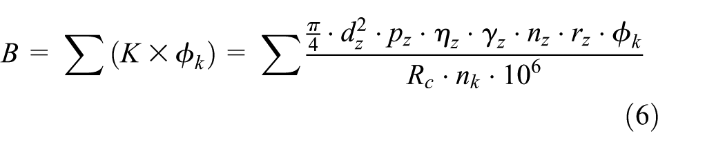
B = \sum (K \times ϕ_{k}) = \sum \frac{\frac{π}{4} \cdot d_{z}^{2} \cdot p_{z} \cdot η_{z} \cdot γ_{z} \cdot n_{z} \cdot r_{z} \cdot ϕ_{k}}{R_{c} \cdot n_{k} \cdot 10^{6}}

(6)

where K is the pressure on the single shoe, φ_k is the nominal friction coefficient and the formula can be queried through the regulations on railway train traction, d_z represents the diameter of the brake cylinder, p_z indicates the air pressure of the brake cylinder, η_z is the transmission efficiency of the braking apparatus, γ_z represents the braking leverage, n_z represents the number of brake cylinders equipped with a train, n_k represents the number of brake shoes installed in a single vehicle, r_z represents the radius of the brake disc, and R_c indicates the radius of the wheel. When the train is selected, it is possible to see that the size of the braking force is merely related to the speed of the train and the relevant operation of the brake.

When the train is running, the locomotive traction is related to the train’s speed under the certain motor parameters. When we calculate the traction force, a certain margin should be taken into account and take 90% of the maximum traction force.

Based on the descriptions above, we know that the train is subjected to a variety of forces at the same time in the process of operation and the actual running state of the train is determined by the co-action of all forces acting on it. The resultant force of the train can be expressed as follows

C = \sum_{i = 1}^{n} F_{q} - \sum_{i = 1}^{n} W_{fi} - \sum_{i = 1}^{n} W_{0 i} - \sum_{i = 1}^{n} B_{i}

(7)

where n is the total number of wagons in the train, C is the resultant force of the train.

During the operation of the train, there is still a rotary motion, and the train’s running time and distance equations are

{\begin{matrix} \int dt = \int \frac{1}{ξ \cdot c} dv \\ \int ds = \int \frac{v}{ξ \cdot c} dv \end{matrix}

(8)

where c is the unit resultant force of the train; S, v, and t denote the running distance, speed, and time, respectively; and $ζ$ is the acceleration coefficient³⁶ as

ζ = \frac{127 M}{M + \sum I / R_{h}^{2}}

(9)

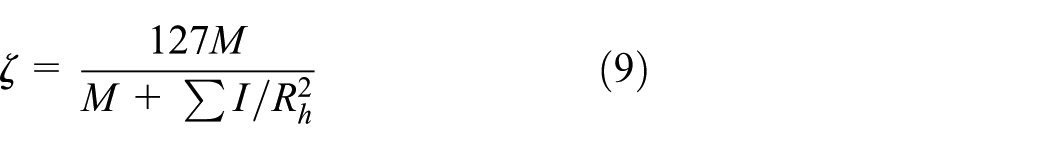
where M is the mass of the whole train, I is the rotational inertia of the rotary motion part, and $R_{h}$ is the radius of gyration of the rotary motion part.

Improved genetic algorithm

Genetic algorithm is based on the operation of all individuals in the population. The algorithm selects individuals based on their individual fitness values in the problem domain, and reengineering methods are borrowed from natural genetics to generate the optimal solution to the problem. This process leads to the evolution of individuals in the population.

The optimal solutions of many nonlinear complex systems can be obtained by genetic algorithm, but in this article, the safe driving curve of the heavy-haul train needs to be obtained. As constraints, a complete interval line data and vehicle information and grouping information, including the speed limit of the line, the line slope, the length of the train, the train traction calculation, and other data, are needed. To avoid the local optimal solution, guarantee the global safe driving strategy, and get the optimal solution of the problem in a reasonable time, an improved genetic algorithm is adopted in this article. Compared with the traditional genetic algorithm, it has the same basic principle, but has been improved in the following aspects:

In this article, we use the strategy of multiple sub-populations to evolve in parallel, the genetic information can be exchanged between the sub-populations, but no interference will occur.³⁷ We obtain the optimal solution of the continuous evolution of sub-populations. Until the condition is satisfied, the optimal solution of all sub-populations is finally compared, and then the global optimal solution is obtained. The superiority of this approach is embodied in the independent evolution of each sub-population so as to ensure the diversity of the population. Even the local optimal solution of the individual population will not have a great impact on the overall results.

Due to the huge amount of the train line data and the train formation information, including the line speed limit, slope, train length, line length, and other data, it is difficult for the algorithm to obtain the result in a reasonable time interval. In this article, we adopt the adaptive adjustment strategy of crossover operator and mutation operator. According to the fitness of each sub-population in the evolutionary process, the crossover probability and mutation probability of the individual within the population are determined. The probability of crossover and mutation operators will become smaller and smaller, so that the proportion of the optimal solution in the population will increase continuously.

In this article, the process of improving genetic algorithm is shown in Figure 3.

Figure 3.

Flow chart of improved genetic algorithm.

The steps of improving genetic algorithm are described below:

Step 1. The parameters needed for the improved genetic algorithm are initialized, such as population size, maximum genetic algebra, the use of the generation gap, the number of species, individual accuracy, the crossover probability of individuals, and individual variation probability.

Step 2. Reading enough traffic data, including the line data (line length, speed data, and slope data) and train data (total weight of the train, train’s locomotive traction, train’s air-braking characteristics, and train marshaling data), and calculating the running equation of the heavy-haul train.

Step 3. Key point code. Runtime state of the heavy-haul train mainly includes four conditions, namely, locomotive traction, coasting, braking resistance, and air braking, which is decided by their switching position. In this article, the train’s running condition is used as the gene to encode, where the sequence of these conditions constitutes the gene of the chromosome. The operating conditions are calculated according to the train’s traction calculation, the running time, and the condition of air brake characteristic. Using real-number encoding, and initializing the train’s conditions of the line, a chromosome represents a control plan with multiple genes to generate an initial population. To ensure the diversity of the populations, each population is randomly generated in the initial conditions, so every working sequence in the population is not same in the initial populations.

Individual genes GK_i represent a condition; its value and working conditions are shown in Table 2.

Table 2.

Corresponding relationship between the train’s working condition and the gene value.

Train’s working condition	Locomotive traction	Coasting	Braking resistance	Air braking
Gene value, GK_i	[0,1)	[1,2)	[2,3)	[3,4)

[0,1), [1,2), [2,3), and [3,4) in Table 2, respectively, represent the locomotive traction condition, coasting condition, braking resistance, and air braking condition of the train. And each condition is calculated as follows.

Assume that the running length of the section is represented by L, and it can be divided into N sections by dividing the position of the transition point.

When GK_i is the air brake condition

{\begin{matrix} a_{i} = (B_{i} + W_{fi} + W_{0 i}) / m \\ v_{(i, 1)} = \sqrt{v_{(i, 0)}^{2} + 2 a_{i} l_{i}} \\ t_{i} = | (v_{(i, 1)} - v_{(i, 0)}) / a_{i} | \end{matrix}

(10)

When GK_i is the coasting condition

{\begin{matrix} a_{i} = (W_{fi} + W_{0 i}) / m \\ v_{(i, 1)} = \sqrt{v_{(i, 0)}^{2} + 2 a_{i} l_{i}} \\ t_{i} = | (v_{(i, 1)} - v_{(i, 0)}) / a_{i} | \end{matrix}

(11)

When GK_i is the locomotive traction condition

{\begin{matrix} a_{i} = (F_{i} - W_{fi} + W_{0 i}) / m \\ v_{(i, 1)} = \sqrt{v_{(i, 0)}^{2} + 2 a_{i} l_{i}} \\ t_{i} = | (v_{(i, 1)} - v_{(i, 0)}) / a_{i} | \end{matrix}

(12)

When GK_i is the braking resistance condition

{\begin{matrix} a_{i} = (B d_{i} + W_{fi} + W_{0 i}) / m \\ v_{(i, 1)} = \sqrt{v_{(i, 0)}^{2} + 2 a_{i} l_{i}} \\ t_{i} = | (v_{(i, 1)} - v_{(i, 0)}) / a_{i} | \end{matrix}

(13)

where F_i is the traction of the train in the ith section, B_i is the air brake force of the train in the ith section, Bd_i is the braking resistance force in the ith section, W_fi is the additional resistance of the train in the ith section, W_0i is the basic resistance of the train in the ith section, a_i is the acceleration of the train in the ith section, v_(i,1) is the end speed of the train in the ith section, v_(i,0)is the initial speed of the train in the ith section, t_i is the train’s running time in the ith section, l_i is the length of the ith section, m is the quality of the train, and i is the ith section of the front line of the train’s running.

Changes in gene values mean changes in conditions. The quality of the gene is evaluated according to the function value of the fitness function.

Step 4. Calculate the fitness function.

To ensure the safe operation of the train, the heavy-haul train in the Shuo Huang Railway needs to adopt the circulating air brake when it is running on a continuously long and steep downgrade. When the train adopts circulating air braking, to ensure enough wind pressure on the next brake and make the train safe to brake next time, we must ensure that the train has enough air-filled time. If there is not enough time to fill the air, it will endanger the safety of the train, so the charge time must be controlled in a reasonable range. Therefore, the train’s running time is regarded as one of the indexes of fitness function. To ensure the safe operation and efficiency of the train, there is a constraint on the position and speed of the relief point and brake point. If the speed of the train in these positions does not meet the constraints, it will directly lead to the overspeed of the train and endanger the safe driving of the train. Therefore, the train’s running speed is used as the index of the fitness function. In this article, the two aspects of the speed and running time of the fitness value are calculated. Any chromosome in the population corresponds to a sequence of train’s working conditions. The quality of the sequence is mainly expressed by the fitness function value of the chromosome. The fitness function is transformed from the objective function. The fitness value represents the probability of the individual to the next generation, so it must be nonnegative.

According to the fitness function of heavy-haul train’s driving strategy, this article mainly calculates the fitness value from two aspects of overspeed and running time.

Overspeed fitness function

To ensure the safety of train’s operation, the train speed should be avoided exceeding the speed limit. To avoid the emergence of speeding queues, the overspeed fitness function is used as the basis for judging the evolutionary process of the population. Therefore, we get the criterion of overspeed fitness function

K_{v} = \sum_{i = 1}^{n} K_{vi}

(14)

K_{vi} = {\begin{matrix} v_{i} - v_{\lim} v_{\lim} \leq v_{i} \\ 0 v_{\lim} > v_{i} \end{matrix}

(15)

where $K_{vi}$ is the index to judge whether each acceleration change point is over speed, $v_{i}$ is the speed at which each acceleration changes, $v_{\lim}$ is the speed limit of each acceleration change point, $n$ is the number of acceleration change points, and $K_{v}$ is the overspeed fitness function value.

2. Running time fitness function

To ensure that the difference between the running time of the train and the running time of the plan is within the allowable range of the error, the difference is taken as the judgment index of the running time fitness function of heavy train

K_{t} = | T_{r} - T_{p} |

(16)

where T_r is the actual running time, T_p is the planned run time, and K_t is the running time fitness function value.

In summary, the two fitness functions have different effects on the control optimization of heavy-haul trains. To take into account both, in this article, the overall fitness function can be expressed as

K = w_{1} K_{v} + w_{2} K_{t}

(17)

Running time and running speed are two different factors, resulting in two optimization directions for the algorithm; the $w_{1}$ and $w_{2}$ are both 0.5 and the weighted sum is 1 using the target weighting method. And the two evolutionary directions have been integrated into one objective function.³⁸

According to the operation evaluation index mentioned above, combined with the running characteristics of heavy-haul train running in a continuously long and steep downgrade, the following optimization model can be established

\min F_{c} = w_{1} \sum_{i = 1}^{n} K_{vi} + w_{2} | T_{r} - T_{p} |

(18)

where $F_{c}$ is the target optimization function.

The constraints are as follows

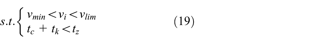
s . t . {\begin{matrix} v_{\min} < v_{i} < v_{\lim} \\ t_{c} + t_{k} < t_{z} \end{matrix}

(19)

where v_min is the minimum release speed for heavy-haul trains. In general, the value is not less than 30 km/h. v_lim is the smaller one in the static speed limit and the temporary speed limit. t_c is the air-filling time of the train pipe, t_k is the empty travel time of the train, and t_z is the time of the increase in train’s speed at which the train is coasting between two braking cycles.

Step 5. Determine whether the iteration termination condition is satisfied. If satisfied, turn to step 7; if not satisfied, turn to step 6.

Step 6. Operator part. First, the number of genetic iteration increases by 1. Second, there are three genetic operators in the calculation, that is, selecting operators, crossover operation, and mutation operation. The selecting operations are based on the individual fitness to determine the genetic opportunity for future generations. The law of individual being selected is as follows

p_{i} = \frac{Fi t_{i}}{\sum_{k = 1}^{n} Fi t_{K}}

(20)

where Fit_i is the fitness value of the individual. Individuals with higher fitness are selected to enter the next generation.

The crossover operation mainly consists of two parts: adaptive crossover rate calculation and crossover calculation.

The calculation of crossover rate P_C is the probability that generations of individual genes are exchanged after two generations of genes, and it will generate two new offspring after the process. With continuous superposition of genetic algebra and optimization of population, the probability of cross breeding among individuals should also be adapted to the change of the evolutionary algebra. In this way, the population has a high convergence rate.

In this article, the calculation formula of P_C is as follows

p_{C} = {\begin{matrix} K_{1} \frac{Fi t_{max} - Fit'}{Fi t_{max} - Fi t_{avg}} & (F' \geq F_{avg}) \\ K_{2} & (F' \leq F_{avg}) \end{matrix}

(21)

where Fit_max is the maximum individual fitness in the current population. Fit_avg is the average fitness of the current population. Fit′ is the larger fitness values between two individuals involved in the crossover operation. K₁ and K₂ are positive constants that cannot be greater than 1. The value of K₂ is relatively large, so that the individuals involved in the crossover operation are more likely to be exchanged. The value of K₁ is relatively small. After the crossover rate is obtained, the crossover calculation can be performed.

The mutation operation includes two parts: adaptive mutation rate calculation and mutation calculation. The calculation of mutation rate P_m is the probability of mutations in alleles in the chromosome, which serves to prevent premature convergence and maintain population diversity. However, with the increase in the number of outstanding individuals within the population, the mutation rate should be gradually adaptive to the change. The calculation formula of P_m is as follows

p_{m} = {\begin{matrix} K_{3} \frac{Fi t_{max} - Fit'}{Fi t_{max} - Fi t_{avg}} & (F' \geq F_{avg}) \\ K_{4} & (F' \leq F_{avg}) \end{matrix}

(22)

where K₃ and K₄ are positive constants that cannot be greater than 1. The value of K₄ is relatively large, which makes an individual, who is involved in the mutation, have a higher probability of being destroyed. The value of K₃ is relatively small.

After the mutation rate is obtained, the individual is subjected to mutation calculation. After three kinds of genetic operators, the population has been evolved, resulting in a new sub-population. And then return to step 4 to calculate the fitness of the individual.

Step 7. Get the current optimal case sequence, then calculate the train’s running equation under this scheme, and get the optimal driving curve of the heavy-haul train.

Research on driving strategy algorithm

In this article, the specific driving strategy research process is shown in Figure 4.

Step 1. Determine whether the train meets the constraint condition (1), if satisfied, proceed to step 2; otherwise, continue to query the judge.

Step 2. Gather the parameters of the train, including the speed, position, traction weight, train’s length information, and air brake information, when the train enters the restraint condition.

Step 3. Collect the line information in front of the train, including line speed limit, temporary speed limit, line slope, length, and other information.

Step 4. The train parameters in step 2 and the line data obtained in step 3 are taken as input parameters to obtain the train’s running equation.

Step 5. The train’s running equation is coded as the key point coding part of the genetic algorithm, and algorithm operations are then performed.

Step 6. After the algorithm is calculated, the optimal operating sequence is obtained.

Step 7. According to the optimal working sequence, the train’s driving curve is drawn.

Step 8. If the request is satisfied, the operation ends, go to the next cycle of control; otherwise, re-cycle.

Figure 4.

Driving strategy flow chart.

In consideration of above situation, it is necessary to consider the following restraint conditions in the process of the heavy-haul train operation

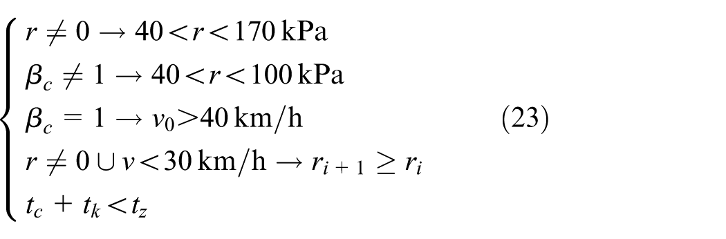
{\begin{matrix} r \neq 0 \to 40 < r < 170 kPa \\ β_{c} \neq 1 \to 40 < r < 100 kPa \\ β_{c} = 1 \to v_{0} > 40 km / h \\ r \neq 0 \cup v < 30 km / h \to r_{i + 1} \geq r_{i} \\ t_{c} + t_{k} < t_{z} \end{matrix}

(23)

In the conditions described above, r is the effective decompression target value and $β_{c}$ is a sign of emergency braking. When the heavy-haul train tube’s pressure is 600 kPa, to reduce the role of the internal longitudinal train force, the effective decompression value, that is, r is 40–170 kPa; when the train is in the usual braking, the decompression value is usually not more than 100 kPa. When applying emergency braking, the initial braking speed, that is, v₀ should not be less than 40 km/h; when braking is carried out and its speed v is less than 30 km/h, no air-filling mitigation action will be performed until parking. t_c is the air-filling time of the train pipe, t_k is the empty travel time of the train, and t_z is the time of the increase in train’s speed at which the train is coasting between two braking cycles.

Simulation cases and result analysis

Simulation parameters

The simulation experiment is realized using MATLAB simulation software. Taking the heavy-haul train as the research object, the driving strategy of the heavy-haul train’s running on the section of the three-aspect automatic block line is studied.

It is known that the length of sections is 25,950 m and the planned operation time is 26 min, that is, 1560 s. The speed that the train runs into the constraint model is set as 64 km/h, and the general decompression value is 50 kPa. First of all, the simulation parameters of the system are collected. According to Figure 3, the parameters mainly include the simulation of the basic line data and train data.

Line data mainly include interval length, line speed limit, line slope, and its length, which are shown in Table 3.

Table 3.

Parameters of the line.

Start point of the grade (m)	End point of the grade (m)	Slope length (m)	Slope value (‰)	Line speed limit (km/h)
0	840	840	−1.5	75
840	1340	500	−5.0	70
1340	1890	550	−1.3	70
1890	2420	530	−9.0	70
2420	2925	505	−10.0	70
2925	3840	915	−6.2	70
3840	16,640	12,800	−10.2	75
16,640	17,190	550	−10.8	75
17,190	17,690	500	−12.0	75
17,690	17,990	300	−10.7	75
17,990	18,990	1000	−12.0	75
18,990	19,740	750	−9.6	75
19,740	21,090	1350	−10.8	75
21,090	21,740	650	−11.3	75
21,740	22,290	550	−10.1	75
22,290	22,540	250	−10.8	75
22,540	23,490	950	−9.4	75
23,490	24,640	1150	−9.4	70
24,640	24,925	285	−11.2	70
24,925	25,245	320	−9.3	70
25,245	25,445	200	−2.0	70
25,445	25,950	505	−1.5	70
25,950				70

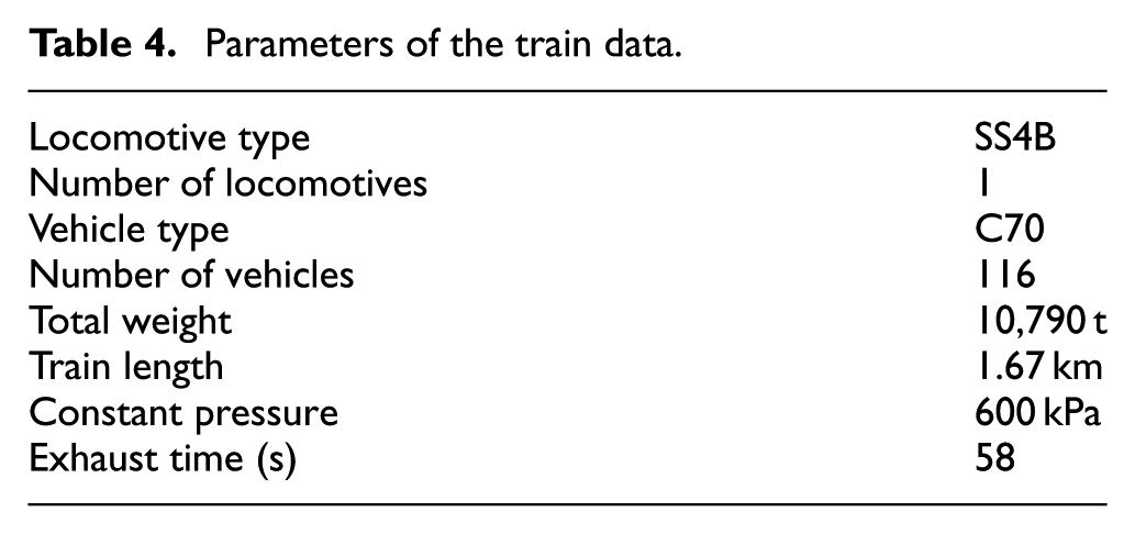
The train data mainly include locomotive and vehicle type, grouping mode, train length, train traction weight, and train pipe constant pressure. The data are shown in Table 4.

Table 4.

Parameters of the train data.

Locomotive type	SS4B
Number of locomotives	1
Vehicle type	C70
Number of vehicles	116
Total weight	10,790 t
Train length	1.67 km
Constant pressure	600 kPa
Exhaust time (s)	58

The control parameters of the genetic algorithm are shown in Table 5.

Table 5.

Improved genetic algorithm parameters.

Control parameters	Parameter value
Maximum hereditary algebra	100
Number of individuals	100
Number of sub-populations	10
Number of bits in a variable	8
Variable dimension	260
Variable range	[0,4]
K ₁	0.5
K ₂	0.85
K ₃	0.02
K ₄	0.05
Time term penalty factor (α)	10,000,000
Over-speed penalty coefficient (β)	10,000,000

Results and analysis

When the train satisfies the constraint condition (1), the above train parameters and the line parameters are used as inputs to calculate the train’s running equation, then the train’s operating equations and the control parameters of the genetic algorithm are brought into the genetic algorithm, and the optimal operation sequence of the train is calculated as shown in Figure 5.

Figure 5.

Optimal solution and ordinal number.

Figure 5 is the optimal solution of genetic algorithm with its sequence number. The figure shows the value of individual genes, corresponding to the value of the train’s running condition. Figure 6 shows the change in the objective function for each generation in the improved genetic algorithm.

Figure 6.

Evolution process.

It can be seen from the graph above that the objective function value of the optimal solution decreases gradually with the increase in the hereditary algebra and remains unchanged from the 12th generation, which shows a good convergence. And it can be seen that the optimal global optimal solution, which satisfies the constraints and requirements, has been optimized by the algorithm.

The final simulation results are shown in Figure 7.

Figure 7.

Simulation curve and driving curve.

In Figure 7, the solid green line is the speed limit of the train line, green dotted line is the forbidden releasing speed, the red curve is the train’s driving curve obtained by the improved genetic algorithm, and the blue curve is the actual operating curve. The actual driving curve is a curve used to guide the actual operation of the driver. And it comes from the data recorded on the site of Shuo Huang Railway in this article. It is a curve that can be verified by the field and can guarantee the safety of train’s running.

There are two or more continuous downgrades in front of the running line, and the train needs a cycle of air braking to adjust speed. To ensure the safety of train’s operation, the speed of the train is forbidden to exceed the speed limit of the line. When the train is relieved, the speed must be greater than 30 km/h. So, the speed of the train is like a saw tooth’s speed profile. The decline in the curve means that the train is executing the braking order, and the speed drops until the relief point. The ascent of the curve means that the train has executed the mitigation order, and the speed is up until the braking point is reached. So, the actual curve is shown in the blue curve.

Result analysis

Figure 8 shows the error contrast between the simulation curve and the actual driving curve.

Figure 8.

Error diagram of simulation curve and driving curve.

Figure 8 shows that the maximum value of the difference between the actual curve and the simulated one is nearly 4 km/h. The detailed comparison can be seen in Table 6.

Table 6.

Comparison of simulation results and real data.

Running distance (m)	Actual speed (km/h)	Simulation speed (km/h)	Difference (km/h)
100	63.23	63.81	−0.58
1100	61.75	61.65	0.1
2100	61.67	61.56	0.11
3100	60.8	62.31	−1.51
4100	62.73	63.29	−0.56
5100	65.2	65.89	−0.69
6100	69.86	69.77	0.09
7100	58.26	55.08	3.18
8100	55.92	57.77	−1.85
9100	64	65.56	−1.56
10,100	71.55	71.77	−0.22
11,100	66.81	65.08	1.73
12,100	49.4	50.57	−1.17
13,100	55.37	55.35	0.02
14,100	63.26	63.2	0.06
15,100	70.81	68.49	2.32
16,100	60.75	91.92	−31.17
17,100	50.42	52	−1.58
18,100	59.71	61.47	−1.76
19,100	68.91	70.13	−1.22
20,100	67.67	65.74	1.93
21,100	55.79	53.11	2.68
22,100	54.43	54.93	−0.5
23,100	60.25	61.38	−1.13
24,100	66.31	65.89	0.42
25,100	60.21	61.23	−1.02
25,950	61.71	63	−1.29

The first column in the table shows the running distance of the heavy-haul train, the second column shows the actual speed of the train at the corresponding distance, and the third column shows the running speed of the train’s simulation corresponding to the second column. From this table, we can obtain the following conclusions: the maximum difference between the two speeds is 3.82 km/h, the mathematical expectation of the speed difference is −0.33146, and the variance is 1.41500. The average running speed of the train is 61.99 and 61.66 km/h, which is calculated by the driving curve and the actual operating curve.

The above calculated data indicate that the difference between the simulated driving curve and the actual curve in the same position is smaller. It can be seen from Figure 7 that the simulation curve and the actual control curve have similar air brake timing, mitigation opportunities, and operating trends.

In addition, to better illustrate the effectiveness of the algorithm, from the algorithm to optimize the target, we compared the simulation data with the actual train’s operation data, as shown in Tables 7 and 8.

Table 7.

Comparison of train’s running time.

Planned run time	Actual running time of train
1560 s	1507 s

Table 8.

Comparison of average speed of train.

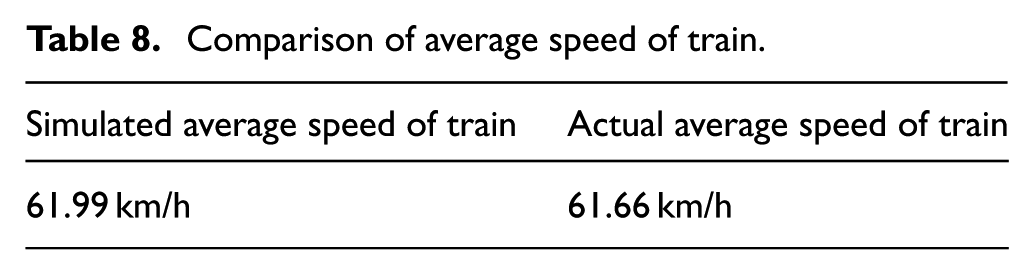
Simulated average speed of train	Actual average speed of train
61.99 km/h	61.66 km/h

From the data of the above two tables, it can be seen that the simulated running time of the train differs from the actual running time by 53 s, and the simulated average speed of the train is 0.33 km/h away from the one of the trains.

It shows that the simulation curve is approximately consistent with the actual curve. It is further shown that the simulation is very effective.

In the same way, to verify the effectiveness of the algorithm, we added another track line, which has positive and negative slope values. Specific line data and simulation analysis are shown in Table 9.

Table 9.

Parameters of the second line.

Start point of the grade (m)	End point of the grade (m)	Slope length (m)	Slope value (‰)	Line speed limit (km/h)
0	500	500	−6	75
500	1008	508	−2	75
1008	2012	1004	1	75
2012	3312	1300	3.5	75
3312	3719	407	6.3	75
3719	4313	594	6	75
4313	4820	507	−3	75
4820	5440	620	2	75
5440	5980	540	1	75
5980	6540	560	−2	75
6540	9100	1081	−2	75
9210	10,100	890	−5.7	75
10,100	10,659	559	−3	75
10,659	12,000	1341	−4.6	75
12,000

The final simulation results are shown in Figure 9.

Figure 9.

Simulation results of the second line.

The green line represents the actual driving curve of the train, and the blue curve represents the simulation curve. The further data of the two curves are compared to Table 10.

Table 10.

Simulation data contrast of the second line.

	Average speed	Average error	Variance of the speed difference	Running time
Actual driving curve	63.634	—	—	678.886
Simulation driving curve	63.188	0.321	0.4674	683.67

The results show that the velocity difference between the two curves is close, and the simulation can calculate the running curve of the train. The effectiveness of the algorithm is further illustrated.

To further illustrate the advantages of the improved genetic algorithm, we use the standard genetic algorithm for the calculation, and the calculation results are shown in Figure 10.

Figure 10.

Standard genetic algorithm curve and actual curve.

In the figure above, the solid green line is the speed limit of the train line, the green dotted line is the forbidden releasing speed, the black curve is the train’s driving curve obtained by the standard genetic algorithm, and the blue curve is the actual operating curve.

Using the data above, the following conclusions can be worked out. The maximum difference between the two speeds is 5.21 km/h, the mathematical expectation of the speed difference is 4.8622, and the variance is 5.6183. The average running speed of the train is 59.80 and 61.66 km/h, which is calculated by the standard genetic algorithm and the actual operating curve.

Table 11 is a comparison of the differences between the two different algorithms and the actual curve.

Table 11.

Comparison of the results of two algorithms.

	Mathematical expectation (km/h)	Variance	Computing time (s)
Improved genetic algorithm	−0.35146	1.41500	4
Standard algorithm	4.8622	5.6183	22

From the above table, the results of the improved genetic algorithm are closer to the actual driving curve. Moreover, the improved algorithm is less time-consuming.

Conclusion

In this article, an improved genetic algorithm based on the train’s running equation is proposed to ensure the safety of running trains in the intervals. This method does not require a large number of actual driving data as the basis. And in this method, the equations of train’s operation and the train’s driving strategies are related to each other. First, according to the line condition and the data of train’s formation, the force analysis of the train’s running process is carried out, then we find the constraint conditions, and establish the train’s operation equation. Second, the train’s running equation is coded to improve genetic algorithm. Finally, the optimal operation sequence is obtained, and we get the optimal train driving strategies to guarantee train’s safety.

According to the calculation results of improved genetic algorithm and standard genetic algorithm, the results of the improved genetic algorithm are more consistent with the actual driving curve. The conclusions are as follows based on the results of the improved genetic algorithm and the actual driving curve.

When the train is running on the line that satisfies the constraint condition (1), the method can be used to obtain the driving curve to ensure the safe operation of the train. The result shows that the maximum value of the difference is 3.82 km/h between the actual curve and the simulated one, and the mathematical expectation of the speed difference is −0.33146, which means that the average speed of both is very close. And the variance of the speed difference is 1.41500, which indicates that the shape of the simulation curve is very close to the actual curve. The train’s simulated running time differs from the actual running time by 53 s. It shows that the simulation results can meet the punctuality rate of trains. In addition, the simulation curve and the actual curve have a similar air brake timing, mitigation opportunities, and operating trends. So, these data prove that our curve can guarantee safety and the method is effective and feasible for practical applications.

Footnotes

Handling Editor: Luis Baeza

Declaration of conflicting interests

The author(s) declared no potential conflicts of interest with respect to the research, authorship, and/or publication of this article.

Funding

The author(s) disclosed receipt of the following financial support for the research, authorship, and/or publication of this article: This work was funded by the Beijing Municipal Natural Science Foundation under grant no. L161008, the Beijing Municipal Science and Technology plan projects under grant nos D151100005815001 and Z161100001016008, Shenhua Group Scientific Research funding projects under grant no. 20140269, and Civil Aviation Science and Technology project under grant no. 201501.

References

Sun

Mao

. Dynamic analysis of heavy haul train. In: China Railway Society of Heavy Haul Train Coupler, Buffer, Brake Symposium, Beijing, 1 August 1985, Beijing: China Railway Society.

Chang

. Differential evolution based tuning of fuzzy automatic train operation for mass rapid transit system. IET Electr Power App 2000; 147: 206–212.

Mitsukawa

. The automatic train operation equipment with expert system. Japan Tappi J 2002; 56: 309–315.

Chen

. Automatic speed control algorithm study based on fuzzy-predictive control logic. Appl Mech Mater 2012; 195–196: 1163–1168.

Qian

. Multi objective train operation optimization based on particle swarm optimization algorithm. J Southwest Jiaotong Univ 2010; 45: 70–75.

Xun

Ning

. Multi-objective optimization method for the ATO system using cellular automata. In: 2008 11th international conference on computer system design and operation in the railway and other transit systems (COMPRA1L08), Toledo, 16–17 September 2008, pp.173–182. Southampton: WIT Press.

Zhao

Gao

. A new control method of automatic train operation in urban rail transit based on improved generalized predictive control theory. In: Proceedings of the 2013 international conference on electrical and information technologies for rail transportation (EITRT2013), Changchun, China, 25–27 October 2013, pp.15–23. Berlin: Springer-Verlag.

Hou

Yin

et al . Terminal iterative learning control based station stop control of a train. Int J Control 2011; 84: 1263–1274.

Yin

Chen

. Intelligent train operation algorithms for subway by expert system and reinforcement learning. IEEE Trans Intell Transp Syst 2014; 15: 2561–2571.

10.

Yang

Liu

et al . Modeling and tracking control of high speed EMU braking process. J China Rail Soc 2016; 3: 80–86.

11.

Lang

Ying

Wang

. Modeling and simulation of high speed train braking and driving simulator. J Tongji Univ: Nat Sci Edi 1994; 2: 39–46.

12.

Song

. Data-based fault-tolerant control of high-speed trains with traction/braking notch nonlinearities and actuator failures. IEEE T Neural Networ 2011; 22: 2250–2261.

13.

. Research and simulation of train automatic driving algorithm based on extenics. J Railway Comput Appl 2013; 22: 1–4.

14.

Feng

. Optimal control of train autopilot system based on LQR algorithm. Southwest Jiaotong University 2014: 1–47.

15.

. Research on automatic train operation simulation based on adaptive control strategy. Beijing Jiaotong University 2013: 1–57.

16.

Sandidzadeh

Shamszadeh

. Improvement of automatic train operation using enhanced predictive fuzzy control method. In: Perpinya

(ed.) Reliability and safety in railway. Rijeka: InTech, 2012, pp.121–140.

17.

. Study on the development of railway heavy haul transportation in China. Rail Transp Econ 2011; 33: 42–46.

18.

Zhu

. Dynamic simulation of urban rail transit train based on single particle model. J Chin Rail Soc 2011; 33: 14–19.

19.

Zhang

. Heavy haul train drivers pragmatic. Chengdu, China: Southwest Jiaotong University Press, 2014.

20.

Chou

Xia

Kayser

. Modelling and model validation of heavy haul trains equipped with electronically controlled pneumatic brake systems. Control Eng Pract 2007; 4: 501–509.

21.

Khmelnitsky

. On an optimal control problem of train operation. IEEE T Automat Contr 2000; 45: 1257–1266.

22.

Wong

. Coast control for mass rapid transit railways with searching methods. IEE P: Elect Pow Appl 2004; 151: 365–376.

23.

Wang

. Intelligent maneuvering simulation of heavy haul train. J China Rail Soc 2009; 1: 17–20.

24.

Huang

Tan

Chen

et al . A neural network driving curve generation method for the heavy-haul train. Adv Mech Eng 2016; 8: 1–14.

25.

Qin

Peng

Zhang

. A robust fault estimation scheme for heavy haul trains equipped with ECP brake systems. In: 26th Chinese control and decision conference (CCDC), Changsha, China, 31 May–2 June 2014, pp.2831–2836. New York: IEEE.

26.

Kang

Research on automatic train driving system based on fuzzy predictive control. Southwest Jiaotong University 2006: 1–69.

27.

Chen

Lin

Block-layout design using MAX-MIN ant system for saving energy on mass rapid transit systems. IEEE T Intell Transp 2009; 10: 226–235.

28.

Lin

Lai

Optimization of train-speed trajectory and control for mass rapid transit systems. Control Eng Pract 2011; 19: 675–687.

29.

Bing

Dong

Zhang

. Speed adjustment braking of automatic train operation system based on fuzzy-PID switching control. In: Sixth international conference on fuzzy systems and knowledge discovery, Tianjin, China, 14–16 August 2009, pp.577–580. New York: IEEE.

30.

Howlett

Cheng

Optimal driving strategies for a train on a track with continuously varying gradient. J Aust Math Soc B 1997; 38: 388–410.

31.

Pudney

Howlett

Optimal driving strategies for a train journey with speed limits. J Aust Math Soc B 1994; 36: 38–49.

32.

Analysis of necessary conditions for the optimal control of a train, vol. 18. Adelaide, SA, Australia: University of South Australia, 2006, pp.139–144.

33.

Zhang

Zhuan

Development of an optimal operation approach in MPC framework for heavy haul trains. IEEE T Intell Transp 2015; 16: 1391–1400.

34.

Zhuan

Xia

Speed regulation with measured output feedback in the control of heavy haul trains. Automatica 2008; 44: 242–247.

35.

Tian

Research on improved adaptive genetic algorithm. J Nanjing U Aeronaut 2006; 2: 19–22.

36.

Zhao

Train traction calculation. Chengdu, China: Southwest Jiaotong University Press, 2013.

37.

Liu

Guo

et al . Study on optimization of energy saving operation of urban rail train based on multi population genetic algorithm. J Syst Simul 2010; 22: 921–925.

38.

. Multi-objective optimization algorithm based on genetic algorithm. Technol Inf 2011; 9: 38.

Research on the driving strategy of heavy-haul train based on improved genetic algorithm

Abstract

Keywords

Introduction

Train’s operation equation and improved genetic algorithm

Train’s operation equation

Improved genetic algorithm

Research on driving strategy algorithm

Simulation cases and result analysis

Simulation parameters

Results and analysis

Result analysis

Conclusion

Footnotes

Declaration of conflicting interests

Funding

References