Sage Journals: Discover world-class research

Abstract

Nowadays, many kinds of flexible manufacturing systems are used to process many complex manufacturing works due to their machine flexibility and routing flexibility. However, such competition (i.e. robots and machines) for shared resources by concurrent job processes can lead to the problem of a system deadlock. In existing researches, almost experts adopted place-based as controllers to solve the deadlock problems of flexible manufacturing systems whatever the concept of siphons or the reachability graph method are used. Among them, only the reachability graph ones can obtain maximally permissive live states. In this article, the authors try to propose one novel transition-based deadlock prevention concept to solve flexible manufacturing system’s deadlock problem. In addition, two algorithms are developed to support above concept. The experimental results indicate that the proposed policy not only can obtain maximally permissive controllers but also recover all original deadlock markings.

Keywords

Deadlock prevention maximally permissive Petri nets flexible manufacturing systems reachability graph

Introduction

Flexible manufacturing systems (FMSs)¹ are a variable working system using all kinds of machines, robots, and conveyors that are shared resources. The FMSs may consider varied resource allocation systems (RASs).² The deadlock occurs if two or more competing actions in shared resources. Thus, engineers must consider and solve the deadlock problems when they want to design and control the deadlock-prone FMS. Petri net^3–8 is good to model and analyze FMSs because of the wonderful dynamic and graphic representation. Therefore, almost researchers use Petri nets as their tool to obtain all kinds of controllers. Furthermore, there are three kinds of controllers used to solve FMS’ deadlock problems. They are control places based on siphon concept,^1,9–14 control places in reachability graph analysis,^15–17 control arcs,² and control transitions.^18–20

Liu et al.⁹ presented a concept of controllable siphon basis that adding a control place and related arcs to each strict minimum siphon forming a controllable siphon basis. A new deadlock prevention policy was proposed by an algorithm for constructing a controllable siphon basis. This novel deadlock prevention policy by controllable siphon basis is better than the elementary siphon algorithm.¹¹ But how to find a controllable siphon basis to get a best performance is a heavy cost to finish in the large Petri net (PN).

Wang et al.¹⁰ proposed an algorithm using an emptied siphon based on loop resource subnets to extract a desired emptied strict minimum siphon (DESMS). Then, they applied the mixed-integer programming (MIP) to obtain a maximally permissive liveness-enforcing supervisor. When one extracts a desire emptied strict minimum siphon, it must be going through three steps of processing. The complexity increases. Although the MIP obtains a maximally permissive liveness-enforcing supervisor, the marking states of PN will be sacrificed some.

Uzam and colleagues^15,16 develop a deadlock prevention policy based on theory of regions to obtain maximal liveness performance. However, the policy fails to determine all sets of event-state-separation-problems (ESSPs), and its application seems limited to some special nets only. Therefore, some works^21–24 aim to develop a computationally more efficient optimal deadlock control policy based on the theory of regions.

Another new method named interval inhibitor arcs² is proposed. Two main stages are present as follows: the first stage is to analyze the reachability graph of PN. The next step is searching the good markings, dangerous markings, bad markings, and dead markings. And, it prevents good markings into the bad markings. Finally, the deadlock system will be live. Note that this approach needs the reachability graph to distinguish the various markings. When the PN system is large, there are too many constraints and variables to consider. Thus, the method is hard likelihood to obtain a live PN. Furthermore, these too many constraints and variables cause not to be an achieved live PN.

Recently, Chen et al.^25,26 propose one novel technology called maximal number of forbidding first bad marking (FBM) problem (MFFP) to obtain optimal states with a small number of control places. It solves the time-consuming problem successfully. According to our survey, the MFFP method seems the best one in existing literature based on place-based controller concept. However, this policy merely can be used in some special nets. For general cases, deadlocks could still exist.

Above means adopt place-based or arcs-based to prevent deadlocks from occurring. The last mean is transition-based controller concept. Huang et al.¹⁸ first used the concept of control transitions to solve the deadlock problem. Advantage of control transition is that it can obtain more permissive markings using state equations.³ However, it is pity that it cannot identify the correct optimal number of reachability graph of one FMS. In following, Zhang and Uzam¹⁹ apply the reachability graph to obtain the control transitions using formulations of the set covering technique.²⁷ However, the efficiency seems too low of the proposed method since it depends on the reachability graph completely. In addition, it also cannot identify the correct optimal number of reachability graph of one FMS in advance.

Based on above disadvantages of two transition-based control policies, this article proposes two improved deadlock prevention policies. The two transition-based deadlock prevention policies not only can identify correct maximally permissive number of reachable markings of one FMS in advance but also recover all original illegal markings.

The rest of this article is organized as follows. Section “Preliminaries” briefly reviews the basic concept of PNs used in this article. Section “The proposed algorithm of transition-based controllers” presents our proposed two transition-based deadlock prevention policies. Section “Examples” gives two examples to test the efficiency of the proposed policy. Section “Conclusion” makes the conclusion.

Preliminaries

One PN original structure is defined as follows.

Definition 1

N = (P, T, F, W), where P = {p₁, p₂, p₃, …, p_m} is a finite, non-empty, and disjoint set of places. T = {t₁, t₂, t₃, …, t_m} is a finite, non-empty, and disjoint set of transitions.^1,3F ⊆ (P×T) ∪ (T × P) is a set of arcs called flow relation. The element F is a set of directed arcs with the arrows from places to transitions or from transitions to places. W(·) is assigned the weight to an arc. Furthermore, the set of arcs in PN are nonnegative integer. A PN n is called ordinary when its weight of arcs is equal to one. Furthermore, for one real FMS net (N) modeled by PN, we called it PN model (PNM). It can be defined as follows.

Definition 2

$PNM = (P_{i} \cup {p_{i}^{0}} \cup P_{Ri}, T_{i}, F_{i})$ , where P_i is the operation place. $p_{i}^{0}$ is the process-idle place. P_Ri is the resource places.²⁸T_i is the set of transitions. F_i is the set of arcs with weight.

Definition 3

Enabling and firing rule:¹⁸ in one PNM, if a node x ∈ P ∪ T, then the preset of node x is defined ^•x = {y ∈ P ∪ T | (y, x) ∈ F}. The post set of node x is defined as x^• = {y ∈ P ∪ T | (x, y) ∈ F}.

A transition t ∈ T is enabled at marking M by iff ∀p ∈ ^•t and M(p) ≥ W(p, t) that will be denoted as M[t>. Afterward firing and enabled a transition t at M will get a new marking M′. It indicates as M[t > M′. A marking M reaches to M′ shown by M[σ > M′ if there exists a firing sequence σ = t₁, t₂, t₃, …, t_n. The set of marking reachable from M in one PNM is called a reachability set as R(N, M₀). The R(N, M₀) is live iff ∀t ∈ T is enabled and dead iff ∃t ∈ T is disabled.

Definition 4

State equation:^3,18 ones write matrix equations, M_k denotes a m × 1 column vector. The entry jth of M_k denotes the token’s number in place j immediately after the firing sequence (kth firing). The kth firing vector u_k is a n × 1 column vector which are n − 1 zeroes and one nonzero entry. The “1” in the ith position indicates that transition i fires at the kth firing. Since the ith row of the incidence matrix A deduces the change in the marking as a result of the firing transition i, we can write the state equation as follows

M_{k} = M_{k - 1} + A^{T} \cdot u_{k}, k = 1, 2, \dots

Definition 5

Necessary reachability condition:^3,18 the assumption that a destination marked M_d is reachable from M₀ by a firing sequence {u₁, u₂, …, u_d}. According to the state equation for i = 1, 2, …, d and summing them, which can be rewritten as follows

A^{T} x = Δ M

where ΔM = M_d − M₀. Here, x is a n × 1 column vector of nonnegative integers that is called the firing-count vector. The ith entry of x deduces the number of times that transition i must fire to change M₀ to M_d.

Definition 6

Livelock:¹⁸x ∈ Z^m, x ≠ 0, is a T-invariant if A^Tx = 0, where x is called the firing-count vector and matrix A denotes the change of the marking. Z^m is the firing set of x.¹¹ One can deduce that a livelock is formed if a reachability graph is not a T-invariant. The characteristic of a livelock marking is not a deadlock and cannot reach the home state.

Definition 7

Reversibility:²⁹

1.A PN N has a home state M_h for an initial state M₀ if for every reachable state M_i ∈ R(N, M₀), a firing sequence σ_i exists such that M_i[σ_i > M_h.

2.A PN N is reversible for an initial state M₀ if M₀ is a home state.

Definition 8

Simple sequential processes with resources (S³PR):¹ An S³PR is defined as the union of a set of nets sharing common places P_Ri, such that $N_{i} = (P_{i} \cup {p_{i}^{0}} \cup P_{Ri}, T_{i}, F_{i} W)$ , where:

Places in P_i are called operation places. P_Ri are called resource ones. ${p_{i}^{0}}$ are called the process-idle places of N_i.

P_i ≠ ∅, p_i⁰ ∉ P_i; P_Ri ≠ ∅, $(P_{i} \cup {p_{i}^{0}}) \cap P_{Ri} = \emptyset$ .

∀p ∈ P_i,∀t ∈ ^•p, ∀t′ ∈ p^•, ^•t ∩ P_R = t′^• ∩ P_R = {r_p}.

∀p ∈ P_i, (^••p ∩ P_R = p ∩ P_R) ∧ (|p^•• ∩ P_R| ≦ 1).

N_i′ is a strongly connected state machine where $N_{i} = (P_{i} \cup {p_{i}^{0}}, T_{i}, F_{i})$ .

Every circuit of N_i′ contains the place $p_{i}^{0}$ , any two N_i′ are composed when they share a set of common resource places P_Ri, $p_{i}^{0}$ is the process-idle place of N_i.

T_i is a finite set of transitions and the function of T_i is defined by W(·).

W(·) is a function defined on the set of transitions.

F_i is the same as the functions I and O describe the input and output arcs of the transitions, respectively.

Definition 9

Saturated number of tokens in idle places: for one real PNM, the size of its reachability graph will become larger when the number of tokens in idle places is adding from small to large. Finally, the number of reachable states will reach to one maximal number whatever the number of tokens increased in idle places. Under the situation, we call the number of tokens saturated number. Please note that the situation also can be called the optimal number of tokens.

For example, in Figure 1, Table 1 shows the different number of tokens in two the idle places (i.e. p₁ and p₆). From Table 1, we can see that the PNM reaches the maximal reachable states when the (p₁, p₆) is (3, 3). The experimental groups 21–24 are just used to present that the maximal reachable states of the PNM are equal to 15. Furthermore, the maximal reachable states are 15 whatever how large number of tokens is added into or increased into the idle place. Therefore, the set of (3, 3) is what we want, it is the saturated number of tokens in idle places of this PNM.

Figure 1.

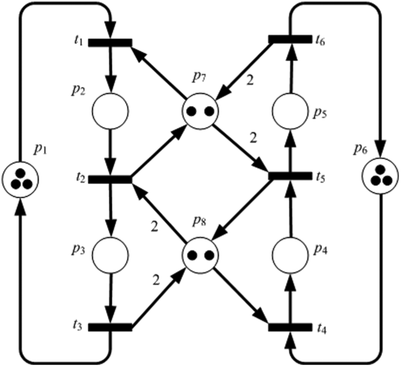
One small Petri net.⁶

Table 1.

The variety of the number of RG when given different number tokens of (p₁, p₆).

Group no.	M(p ₁)	M(p ₆)	Number of RGs	Group no.	M(p ₁)	M(p ₆)	Number of RGs
1	1	0	3	13	1	3	10
2	2	0	5	14	1	4	10
3	3	0	6	15	2	1	9
4	4	0	6	16	2	2	13
5	5	0	6	17	2	3	14
6	0	1	3	18	2	4	14
7	0	2	5	19	3	1	10
8	0	3	6	20	3	2	14
9	0	4	6	21	3	3	15
10	0	5	6	22	3	4	15
11	1	1	6	23	4	4	15
12	1	2	9	24	5	5	15

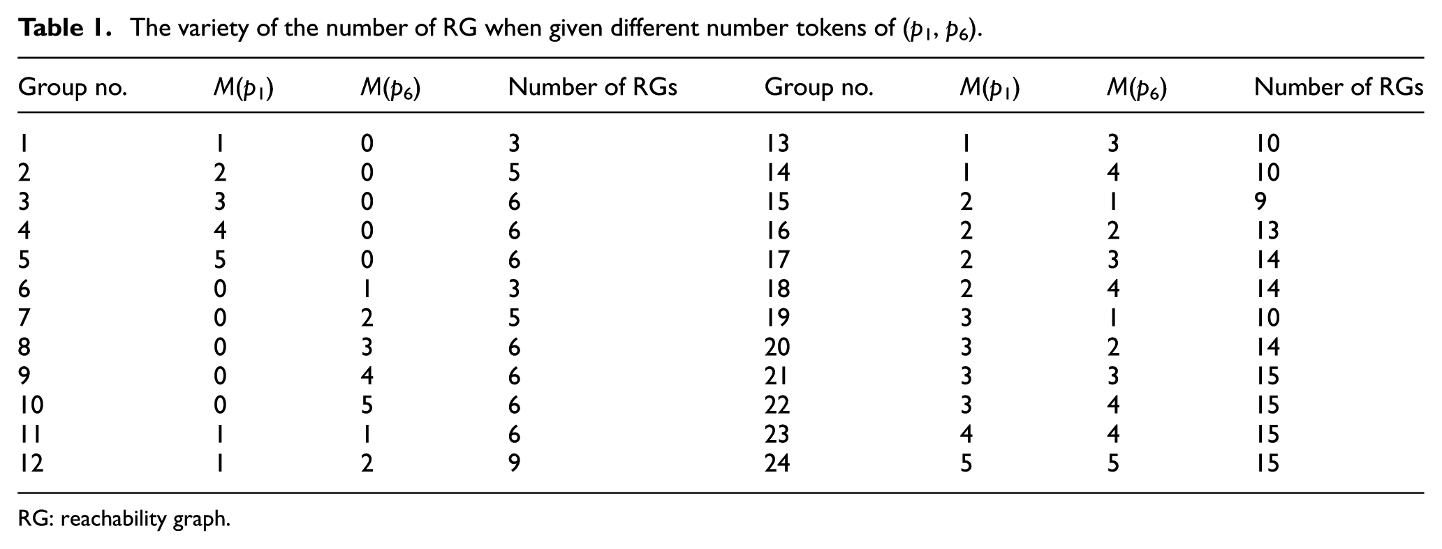
RG: reachability graph.

Definition 10

The first deadlock marking (FDM): based on Definition 9, for one real PNM, one deadlock marking appear first in this system while the number of tokens for idle places is adding from small to large. The deadlock marking is defined as the FDM.

The proposed algorithm of transition-based controllers

In this section, two novel algorithms based on control transitions will be developed. Please note that the proposed algorithms can not only solve the deadlock problem but also recover all original markings of one PNM whatever they are live or deadlock initially. In other words, in this article, the so-called “maximally permissive states” means that all original deadlock markings can be further recovered under the proposed algorithms. Please also note that under the two algorithms, the saturated number of tokens in one PNM’s idle places can be identified. Therefore, the maximal reachable markings of one PNM’s reachability graph can then calculated correctly. Huang et al.’s¹⁸ deadlock prevention policy just uses the dead marking and the initial marking to calculate the control transition. In other words, it does not know what the saturated number of tokens is. In this article, we can identify the correct and maximal number of one PNM’s reachable markings once the framework is established.

One small typical example⁶ shown in Figure 1 is used to illustrate the proposed algorithms. In Figure 1, one can see that there are two idle places (i.e. p₁ and p₃) in this PNM, and their saturated or called optimal value is equal to 3. Under this situation, the number of its reachable markings shown in Figure 2 is equal to 15. Please note that there are four illegal markings (i.e. three quasi-dead markings and one deadlock marking) in the reachability graph. The detailed information is shown in Tables 1 and 2, respectively.

Table 2.

The property of all reachable markings of Figure 2.

Marking no.	Classification	Information of marking
M ₀	Initial marking	M ₀ = 3p₁+3p₆+3p₇+2p₈
M ₁	Live marking	M ₁ = 2p₁+p₂+3p₆+p₇+2p₈
M ₂	Live marking	M ₂ = p₁+2p₂+3p₆+2p₈
M ₃	Live marking	M ₃ = p₁+p₂+p₃+3p₆+p₇
M ₄	Live marking	M ₄ = 2p₂+p₃+3p₆
M ₅	Quasi-dead marking	M ₅ = p₁ + 2p₂ + p₄ + 2p₆ + p₈
M ₆	Deadlock marking	M ₆ = p₁ + 2p₂ + 2p₄ + p₆
M ₇	Live marking	M ₇ = 2p₁+p₃+3p₆+2p₇
M ₈	Quasi-dead marking	M ₈ = 2p₁ + p₂ + p₄ + 2p₆ + p₇ + p₈
M ₉	Quasi-dead marking	M ₉ = 2p₁ + p₂ + 2p₄ + p₆ + p₇
M ₁₀	Live marking	M ₁₀ = 3p₁+p₄+2p₆+2p₇+p₈
M ₁₁	Live marking	M ₁₁ = 3p₁+2p₄+p₆+2p₇
M ₁₂	Live marking	M ₁₂ = 3p₁+p₄+p₅+p₆+p₈
M ₁₃	Live marking	M ₁₃ = 3p₁+2p₄+p₅
M ₁₄	Live marking	M ₁₄ = 3p₁+p₅+2p₆+2p₈

Figure 2.

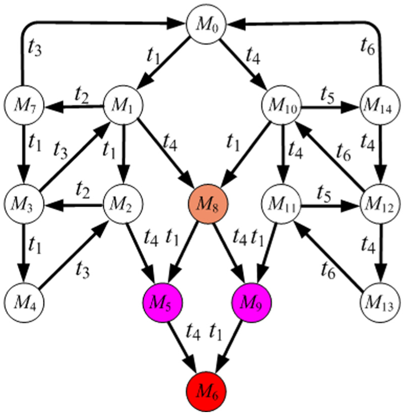
The reachability graph of Figure 1.

Transition-based controllers

Based on Definition 4, one formalized equation for seeking transition-based controllers is developed. First, recall the Definition 4, the state equation is M_k = M_k_− 1+A^T·u_k. Besides, it is assumed that a deadlock-prone PNM should contain at least one deadlock marking M_d in its reachability graph at which no transition is enabled. Therefore, Definition 4 can be replaced to M_d = M₀+A^T·u_d for a deadlock-prone PNM. Please note that M₀ is initial marking, A is the incidence matrix of a deadlock-prone PNM, and u_d is the firing sequence from M₀ to M_d. As a result, one must find another relatively firing sequence from M_d to M₀ as follows: M_d − A^T·u_d = M₀. The equation can be rearranged to M₀ = M_d − A^T·u_d. Then M₀ = M_d+A^T·(−u_d). Let y_d = −u_d. Then, one can obtain the new state equation for calculating transition-based controllers of a deadlock-prone PNM as follows

M_{0} = M_{d} + A^{T} \cdot (y_{d})

(1)

From above equation, undoubtedly, one can identify one set of firing sequence such that M_d can be recovered.

Two algorithms based on different viewpoints

Two algorithms based on different viewpoints are present as follows:

Algorithm 1: based on the all reachability graph viewpoint.

First, from Figure 2 and Table 2, one can identify that the property of the initial marking and the deadlock marking are M₀ = 3p₁+3p₆+2p₇+2p₈ and M₆ = p₁+2p₂+2p₄+p₆, respectively. Therefore, according to definitions 4 and 5, the control transition equation (CTE) can be listed as follows: M_h = M_d+(O(T_cx) − I(T_cx)). Thus, the output control transition is O(t₇) = 2p₁+2p₆+2p₇+2p₈ and the input control transition is I(t₇) = 2p₂+2p₄. When the set of control transition is put into the original PNM shown in Figure 3, all 15 reachable markings including the 4 illegal markings are live shown in Figure 4.

Figure 3.

A live Petri net system based on Algorithm 1.

Figure 4.

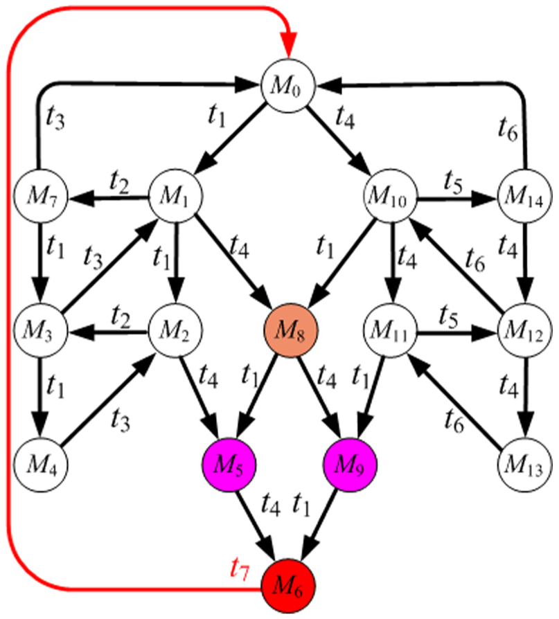
The reachability graph of Figure 3.

Algorithm 2: based on the FDM viewpoint.

In the following, according to Definition 10 one can identify that the system meets the FDM while the two idle places (p₁, p₆) are given (1, 1). The detailed information is shown in Tables 1 and 3.

Table 3.

The property of all reachable markings of Figure 5.

Marking no.	Classification	Information of marking
M ₀	Initial marking	M ₀ = p₁+p₆+2p₇+2p₈
M ₁	Live marking	M ₁ = p₂+p₆+p₇+2p₈
M ₂	Live marking	M ₂ = p₃+p₆+2p₇
M ₃	First deadlock marking (FDM)	M ₃ = p₂ + p₄ + p₇ + p₈
M ₄	Live marking	M ₄ = p₁+p₄+2p₇+p₈
M ₅	Live marking	M ₅ = p₁+p₅+2p₈

Based on Table 2, one can realize that the saturated number of the two idle places (p₁, p₆) is (3, 3). It means that the maximal number of the reachability graph of the PNM is equal to 15 whatever how many tokens are added into (p₁, p₆). This is also called the full reachability graph viewpoint. On the contrary, in Algorithm 2, we just check when the first one deadlock marking will be produced by the PNM. Since the 12th group starts to produce the FDM, we use its data to calculate the controller. From Table 3, one can identify the deadlock marking is M₃, and its property is p₂+p₄+p₇+p₈. Besides, the property of the initial marking M₀ is p₁+p₆+2p₇+2p₈. From CTE, one can obtain the output control transition O(t₈) = p₁+p₆+p₇+p₈ and the input control transition I(t₈) = p₂+p₄. The PNM is deadlock-free when we put the controller into it. Figures 5 and 6 show the results.

Figure 5.

A live Petri net system based on Algorithm 2.

Figure 6.

The reachability graph of Figure 5.

Algorithms 1 and 2 present the very different viewpoints. Furthermore, Algorithm 1 adopts the viewpoint of global framework. However, Algorithm 2 adopts the viewpoint of local framework. Whatever what viewpoint is adopted, the PNM will be live and can also hold the maximally permissive states. More important, both of the proposed algorithms recover the all deadlock markings.

Theorem 1

Proposed algorithms can recover the deadlock PNM and is maximally permissive.

Proof

According to equation (1), one set firing sequence must exist, such that, M_d can be led back to M₀ once controllers exist. And, the controllers will not make the dead markings vanished. Therefore, the proposed algorithms can recover the deadlock PNM and is maximally permissive.

Examples

In this section, we want to present the high efficiency of the two proposed algorithms by testing two classical examples.^15,18 The first example is used to present the proposed algorithms and the second example is used to make comparison with previous literature. First of all, two deadlock prevention policies are listed based on the two algorithms as follows.

Deadlock Prevention Policy I.

Step 1: Input one deadlock-prone PNM

Step 2: Identify saturated number of idle places

Step 3: Run its full RG based on saturated number of idle places

Step 4: Identify the properties of initial and all deadlock markings

Step 5: Calculate all the controllers based on CTE

Step 6: Add controllers into the deadlock-prone PNM

Step 7: Output one deadlock-free PNM

Deadlock Prevention Policy II.

Step 1: Input one deadlock-prone PNM

Step 2: Run partial RG until the first deadlock marking (FDM) is produced

Step 3: Identify the properties of initial and first deadlock markings

Step 4: Calculate the controller based on CTE

Step 5: Add the controller into the deadlock-prone PNM

Step 6: Repeat steps 2–5 until initial reachable markings are live

Step 7: Output one deadlock-free PNM

In the following, we use example 1 to test the proposed Deadlock Prevention Policies I and II. Figure 7 shows its PNM. According to the Deadlock Prevention Policy I. The full reachability graph is surely needed to run. Figure 8 presents the full reachability graph of Figure 7.

Figure 7.

One classical S³PR system.^15,16

Figure 8.

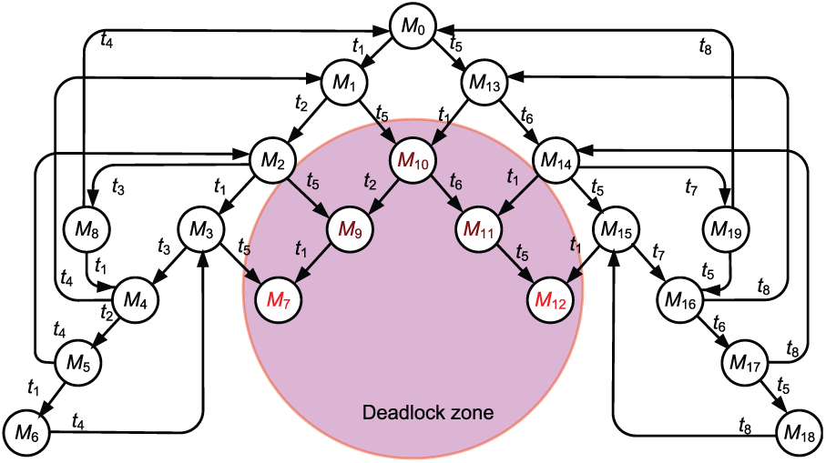
The full reachability graph of Figure 7.

Due to the limitation of paper space, we just show the properties of initial markings and two deadlock markings in Table 4.

Table 4.

The properties of initial and two deadlock markings based on Algorithm 1.

Marking no.	Classification	Information of Marking
M ₀	Initial marking	M ₀ = 3p₁+p₃+p₆+p₉+3p₁₁
M ₇	Deadlock marking	M ₇ = p₁+p₂+p₅+p₁₀+2p₁₁
M ₁₂	Deadlock marking	M ₁₂ = 2p₁+p₂+p₇+p₁₀+p₁₁

Then, we can obtain two controllers t₉ and t₁₀ based on Table 4 and the CTE. The detailed information of t₉ and t₁₀ are I(t₉) = p₂+p₅+p₁₀, O(t₉) = 2p₁+p₃+p₆+p₉+p₁₁, and I(t₁₀) = p₂+p₇+p₁₀, O(t₁₀) =p₁+p₃+p₆+p₉+2p₁₁, respectively. When the set of control transition is put into the original PNM of Figure 7, all 20 reachable markings including the 5 illegal markings (i.e. M₇, M₉, M₁₀, M₁₁, and M₁₂) are live (please refer to Figures 9 and 10).

Figure 9.

The two controllers are added into the PNM of Figure 7 based on Algorithm 1.

Figure 10.

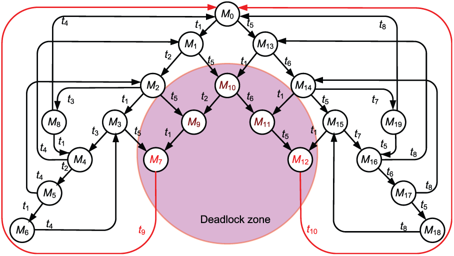
The full live reachability graph of Figure 8 based on Algorithm 1.

In the following, we adopt Deadlock Prevention Policy II to test the example 1. The system meets two FDM while the two idle places (p₁, p₁₁) are given (1, 1). The detailed information is shown in Tables 5.

Table 5.

The properties of initial and two deadlock markings based on Algorithm 2.

Marking no.	Classification	Information of marking
$M'_{0}$	New initial marking	M ₀ = p₁+p₃+p₆+p₉+p₁₁
M_D ₁	First deadlock marking	M_D ₁ = p₃+p₅+p₁₀
M_D ₂	First deadlock marking	M_D ₂ = p₂+p₇+p₉

Similarly, we can obtain two controllers t₁₁ and t₁₂ based on Table 5 and the CTE. The detailed information of t₁₁ and t₁₂ are I(t₁₁) = p₅+p₁₀, O(t₁₁) = p₁+p₆+p₉+p₁₁, and I(t₁₂) = p₂+p₇, O(t₁₂) = p₁+p₃+p₆+p₁₁, respectively. Please notice that, when the two sets of control transition are put into the original PNM of Figure 7, all 20 reachable markings (also including the 5 illegal markings) are live (please refer to Figures 11 and 12).

Figure 11.

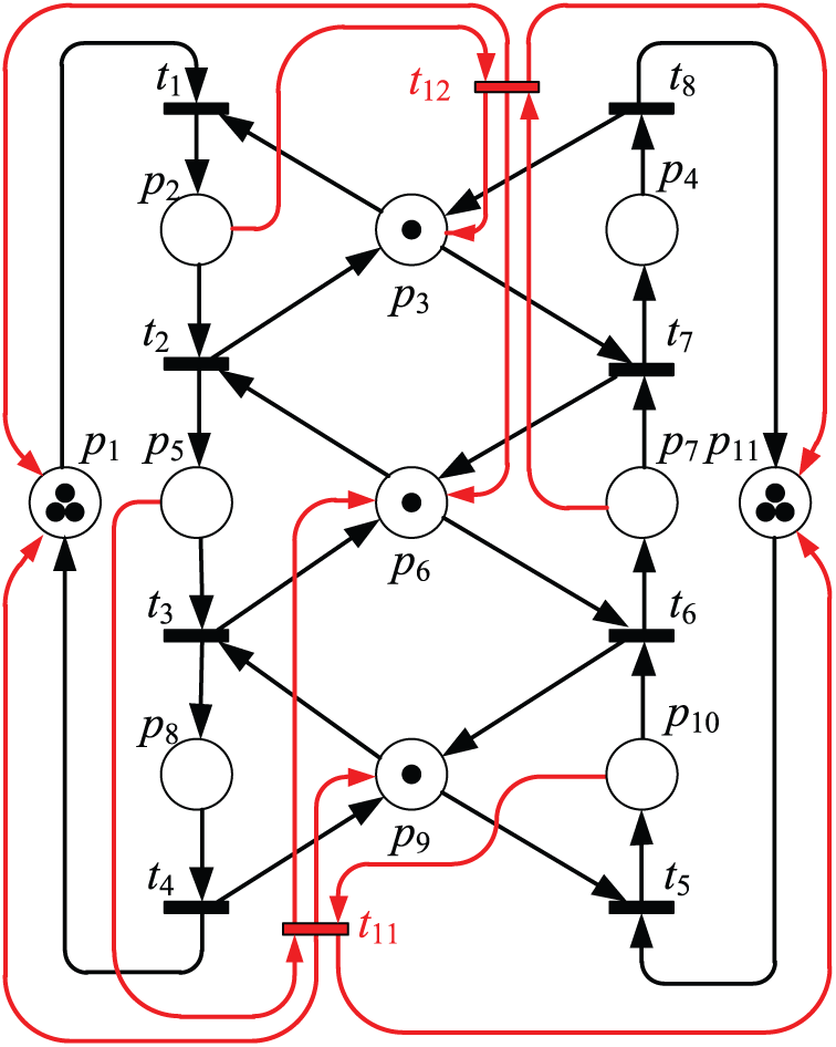
The two controllers are added into the PNM of Figure 7 based on Algorithm 2.

Figure 12.

The full live reachability graph of Figure 8 based on Algorithm 2.

The second example shown in Figure 13 is from Huang et al.¹⁸ and Zhang and Uzam.¹⁹ Huang et al.¹⁸ identify 32 reachable markings including 4 deadlock markings (e.g. 2p₀+p₅+p₆+p₈+p₉, p₀+p₂+p₆+p₈+p₉, p₂+p₃+p₈+p₉, and p₀+p₃+p₅+p₈+p₉). Finally, they recover all reachable markings by their two control transitions (I(t_i) = 2p₇+p₁₁+p₁₂ and O(t_i) = p₈+p₉; I(t_j) = p₇+p₁₀+p₁₁ and O(t_j) = p₈+p₉).

Figure 13.

The second example from the literature.^18,19

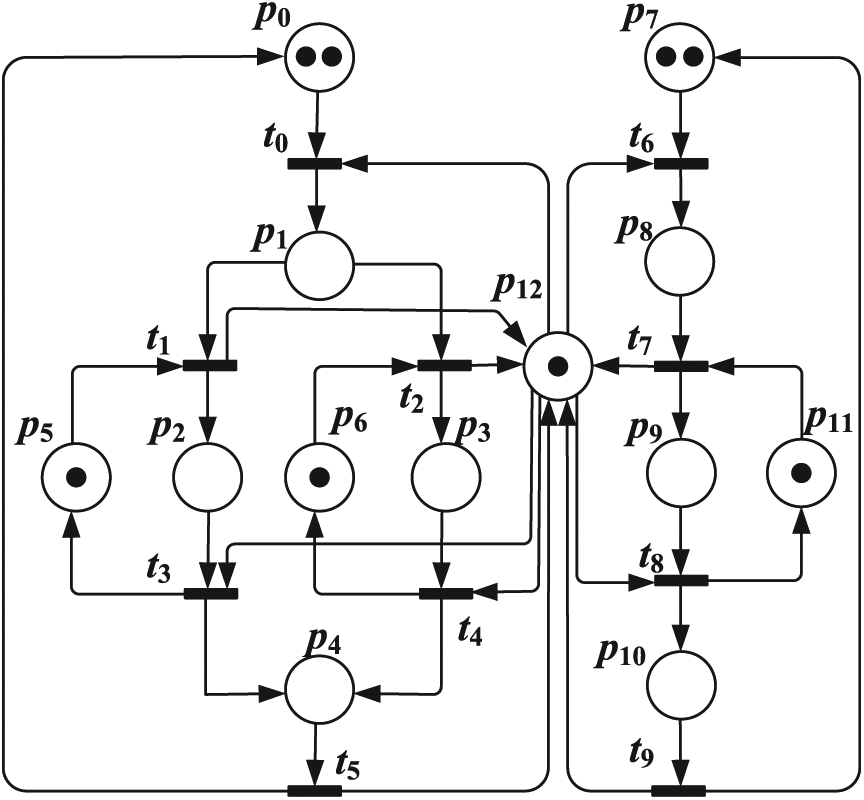
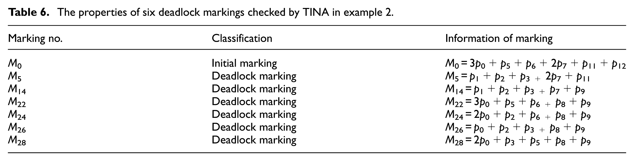
Zhang and Uzam¹⁹ discover a set covering problem and obtain two control transitions to solve the deadlock problem of this example. They also use two same transition-based controllers to make the system deadlock-free. However, in example 2, in fact, according to our study in this article, there should be 34 reachable markings including 6 deadlock markings (shown in Table 6) when the idle places (p₀, p₇) are equal to (3, 2). Furthermore, saturated number of tokens in idle places for example 2 should be (3, 2). Please note that the six deadlock markings are checked by famous software TINA.³⁰ Due to the limitation of paper space, we just show the property of the 6 deadlock markings.

Table 6.

The properties of six deadlock markings checked by TINA in example 2.

Marking no.	Classification	Information of marking
M ₀	Initial marking	M ₀ = 3p₀+p₅+p₆+2p₇+p₁₁+p₁₂
M ₅	Deadlock marking	M ₅ = p₁+p₂+p₃ ₊ 2p₇+p₁₁
M ₁₄	Deadlock marking	M ₁₄ = p₁+p₂+p₃ ₊ p₇+p₉
M ₂₂	Deadlock marking	M ₂₂ = 3p₀+p₅+p₆ ₊ p₈+p₉
M ₂₄	Deadlock marking	M ₂₄ = 2p₀+p₂+p₆ ₊ p₈+p₉
M ₂₆	Deadlock marking	M ₂₆ = p₀+p₂+p₃ ₊ p₈+p₉
M ₂₈	Deadlock marking	M ₂₈ = 2p₀+p₃+p₅+p₈+p₉

Finally, two controllers (I(t₁₃) = p₈+p₉, O(t₁₃) = 2p₇+p₁₁+p₁₂, and I(t₁₄) = p₁+p₂+p₃, O(t₁₄) = 3p₀+p₅+p₆+p₁₂) are hence obtained under the proposed Deadlock Prevention Policy II, and all 34 reachable markings are recovered when the two controllers are added into example 2.

Conclusion

In the existing literature, almost all researches adopt place-based deadlock prevention method to solve the FMS deadlock problem. However, they cannot obtain real maximally permissive controllers since some bad and deadlock markings could not be recovered in the process of controlling FMS. Based on above reason, this research presents one novel deadlock recovery policy using transition-based technology. The proposed policy is obvious better than all existing literatures even all publishing transition-based deadlock prevention policies. Moreover, the proposed policy not only obtains maximally permissive controllers but also recovers all original deadlock markings. Preciously, we can make all markings alive whatever they initially belong to deadlock or illegal ones. In other words, this work is the innovation in deadlock prevention domain. In future works, we will use the proposed policy to test all kinds of FMS or a larger PNM.

Footnotes

Handling Editor: Artde Lin

Declaration of conflicting interests

The author(s) declared no potential conflicts of interest with respect to the research, authorship, and/or publication of this article.

Funding

The author(s) received no financial support for the research, authorship, and/or publication of this article.

ORCID iD

Yen-Liang Pan

References

Ezpeleta

Colom

Martinez

A Petri net based deadlock prevention policy for flexible manufacturing systems. IEEE T Robotic Autom 1995; 11: 173–184.

Chen

Barkaoui

et al . New Petri net structure and its application to optimal supervisory control: interval inhibitor arcs. IEEE T Syst Man Cy A 2014; 44: 1384–1400.

Murata

Petri nets: properties, analysis and applications. Proc IEEE 1989; 77: 541–580.

Zhou

MC.

Deadlock resolution in automated manufacturing systems: Petri net approach. London: Springer-Verlag, 2009.

Zhou

MC.

Elementary siphons of Petri nets and their application to deadlock prevention in flexible manufacturing systems. IEEE T Syst Man Cy A 2004; 34: 38–51.

Huang

Jeng

Xie

et al . Siphon-based deadlock prevention policy for flexible manufacturing systems. IEEE T Syst Man Cy A 2006; 36: 2152–2160.

Zhou

MC.

On siphon compution for deadlock control in a class of Petri nets. IEEE T Syst Man Cy A 2008; 38: 1348–1350.

Wang

Xing

et al . Research on finding elementary siphon in class of Petri nets. Comm Com Inf Sc 2012; 289: 435–442.

Liu

Xing

et al . Deadlock prevention for flexible manufacturing systems via controllable siphon basis of Petri nets. IEEE T Syst Man Cyb 2015; 45: 519–529.

10.

Wang

Zhou

WH.

Design of a maximally permissive liveness-enforcing supervisor with reduced complexity for automated manufacturing systems. Asian J Control 2015; 17: 190–201.

11.

Zhou

MC.

Clarifications on the definitions of elementary siphons in Petri nets. IEEE T Syst Man Cy A 2006; 36: 1227–1229.

12.

Piroddi

Cordone

Fumagalli

Selective siphon control for deadlock prevention in Petri nets. IEEE T Syst Man Cy A 2008; 38: 1337–1348.

13.

Piroddi

Cordone

Fumagalli

Selective siphon control for deadlock prevention in Petri nets. IEEE T Syst Man Cy A 2008; 38: 1337–1348.

14.

Huang

Jeng

Xie

et al . Deadlock prevention policy based on Petri nets and siphons. Int J Prod Res 2001; 39: 283–305.

15.

Uzam

An optimal deadlock prevention policy for flexible manufacturing systems using Petri net models with resources and the theory of region. Int J Adv Manuf Tech 2002; 19: 192–208.

16.

Uzam

Zhou

MC.

An iterative synthesis approach to Petri net-based deadlock prevention policy for flexible manufacturing systems. IEEE T Syst Man Cy A 2007; 37: 362–371.

17.

Ghaffari

Rezg

Xie

XL.

Design of a live and maximally permissive Petri net controller using the theory of regions. IEEE T Robotic Autom 2003; 19: 137–142.

18.

Huang

Y-S

Pan

Y-L

P-J.

Transition-based deadlock detection and recovery policy for FMSs using graph technique. ACM T Embed Comput S 2013; 12: 11.

19.

Zhang

Uzam

Transition-based deadlock control policy using reachability graph for flexible manufacturing systems. Adv Mech Eng 2016; 8: 1–9.

20.

Pan

Tseng

Row

TC.

Design of improved optimal or suboptimal deadlock prevention for FMSs based on place invariant and reachability graph analysis methods. J Algorithm Comput Technol 2017; 11: 261–270.

21.

Pan

Huang

Jeng

et al . Enhancement of an efficient control policy for FMSs using the theory of regions and selective siphons method. Int J Adv Manuf Technol 2013; 66: 1805–1815.

22.

Pan

Huang

Weng

et al . Computationally improved optimal control methodology for linear programming problems of flexible manufacturing systems. J Appl Math 2013; 2013: 294835.

23.

Huang

Pan

YL.

An improved maximally permissive deadlock prevention policy based on the theory of regions and reduction approach. IET Control Theory A 2011; 5: 1069–1078.

24.

Huang

Pan

Zhou

Computationally improved optimal deadlock control policy for flexible manufacturing systems. IEEE T Syst Man Cy A 2012; 42: 404–415.

25.

Chen

Zhou

MC.

Behaviorally optimal and structurally simple liveness–enforcing supervisors of flexible manufacturing systems. IEEE T Syst Man Cy A 2012; 42: 615–629.

26.

Chen

Khalgui

et al . Design of a maximally permissive liveness-enforcing Petri net supervisor for flexible manufacturing systems. IEEE T Autom Sci Eng 2011; 8: 374–393.

27.

Caprara

Fischetti

Toth

A heuristic method for the set covering problem. Oper Res 1999; 47: 730–743.

28.

Marsan

Balbo

Conte

et al . Modeling with generalized stochastic Petri nets. New York: John Wiley & Sons, 1995.

29.

David

Alla

Discrete, continuous and hybrid Petri nets. Berlin: Springer Verlag, 2005.

30.

TINA (Time Petri Net Analyzer) has been developed in the OLC then VerTICS, research groups of LAAS/CNRS, http://projects.laas.fr/tina//download.php

Group no.	M(p ₁)	M(p ₆)	Number of RGs	Group no.	M(p ₁)	M(p ₆)	Number of RGs
1	1	0	3	13	1	3	10
2	2	0	5	14	1	4	10
3	3	0	6	15	2	1	9
4	4	0	6	16	2	2	13
5	5	0	6	17	2	3	14
6	0	1	3	18	2	4	14
7	0	2	5	19	3	1	10
8	0	3	6	20	3	2	14
9	0	4	6	21	3	3	15
10	0	5	6	22	3	4	15
11	1	1	6	23	4	4	15
12	1	2	9	24	5	5	15

Group no.	M(p ₁)	M(p ₆)	Number of RGs	Group no.	M(p ₁)	M(p ₆)	Number of RGs
1	1	0	3	13	1	3	10
2	2	0	5	14	1	4	10
3	3	0	6	15	2	1	9
4	4	0	6	16	2	2	13
5	5	0	6	17	2	3	14
6	0	1	3	18	2	4	14
7	0	2	5	19	3	1	10
8	0	3	6	20	3	2	14
9	0	4	6	21	3	3	15
10	0	5	6	22	3	4	15
11	1	1	6	23	4	4	15
12	1	2	9	24	5	5	15

Maximally permissive deadlock prevention policies for flexible manufacturing systems using control transition

Abstract

Keywords

Introduction

Preliminaries

Definition 1

Definition 2

Definition 3

Definition 4

Definition 5

Definition 6

Definition 7

Definition 8

Definition 9

Definition 10

The proposed algorithm of transition-based controllers

Transition-based controllers

Two algorithms based on different viewpoints

Theorem 1

Proof

Examples

Conclusion

Footnotes

Declaration of conflicting interests

Funding

ORCID iD

References

Group no.	M(p ₁)	M(p ₆)	Number of RGs	Group no.	M(p ₁)	M(p ₆)	Number of RGs
1	1	0	3	13	1	3	10
2	2	0	5	14	1	4	10
3	3	0	6	15	2	1	9
4	4	0	6	16	2	2	13
5	5	0	6	17	2	3	14
6	0	1	3	18	2	4	14
7	0	2	5	19	3	1	10
8	0	3	6	20	3	2	14
9	0	4	6	21	3	3	15
10	0	5	6	22	3	4	15
11	1	1	6	23	4	4	15
12	1	2	9	24	5	5	15