This article formulates the properties of achievable consensus of linear interconnected discrete systems with multiple internal and external point delays. The formulation is stated in an algebraic generic context as the ability of achievement of (a non-necessarily zero) finite-time common error between the various subsystems. The consensus signals are generically defined so that they can be, in general, distinct of the output or state components. However, the consensus signals of all the interconnected subsystems have the same dimension for coherency reasons. A particular attention is paid to the case of weak interconnection couplings in both the open-loop case and the closed-loop one under, in general, linear output feedback. Some further extensions are given related to consensus over intervals and related to consensus of positive interconnected systems.
The so-called “consensus objective” between a set of agents integrated in networked multi-agent systems is of usefulness in relevant problems like formation flight of unmanned air vehicles, clusters of satellites, self-organization, auto-matched highway systems, congestion control in communication networks, and others.1 A typical example of consensus in dynamic interconnected subsystems is that being reached by a set of coupled oscillators satisfying Kuramoto’s model.2,3 However, a quantized consensus problem of undirected time-varying graphs is proposed while a protocol with fast convergence time to consensus points is used for that purpose.4 In Philip Chen et al.,5 an observer-based adaptive back-stepping scheme is proposed for multi-agent consensus, while a nonlinear consensus protocol for optimal distributed networks of dynamic agents is proposed and discussed in Bauso et al.6 In Li et al.,7 each agent within the multi-agent structure shares information with a subset of the remaining agents. In Zhu and colleagues,8–10 a consensus of fractional-order multi-agent systems is reached via observer-type protocols while the consensus objective is formulated for multi-agent fuzzy dynamic systems with dropout compensation in Han et al.11 It can be pointed out that there are apparent conceptual differences between the consensus objective and the master–slave objective. In particular, in the first case, no particular agent drives its counterparts toward a common consensus objective which is reached by sharing the available information and taking the needed driving actions governed by the appropriate protocols. However, in master–slave problems, the master agent decides the objective to be also reached by the slaves. The achievement of consensus between a set of measurable signals of a system, typically associated with subsystems with the range of agents, or between a vector of measurements of several interconnected systems is receiving important attention in the last years. The deterministic-type consensus objective is generally understood as the asymptotic achievement of zero error between the measurable signals where consensus is claimed. There are also many stochastic-type consensus variants available in the background literature where the defined consensus signals mutually track each other with probability one. In this article, the consensus objective is stated for discrete systems as follows in the most general case: (1) a finite-time deterministic objective in a discrete time-varying linear control system; (2) the error between the various relevant candidate signals for consensus is neither necessarily zero nor identical to any non-zero prefixed value for each pair of compared signals; (3) the various signal candidates for the consensus achievement are not necessarily state or output components of the various subsystems in the interconnected structure; (4) the discrete system can be subject to internal and external commensurate delays; and (5) the problem treatment is based on algebraic tools. In fact, they can consist of linear combinations of measurable signals according to design needs. The above issues are the main contributions of this article related to the background literature and they are developed based on algebraic tools including formal comparisons with controllability and output controllability.
This article is organized as follows. Section “Problem formulation” gives the various concepts and results on finite-time consensus for a linear time-varying discrete system consisting of several coupled subsystems with eventual internal and external point delays. It is not assumed in the general case that either the initial conditions or the consensus error are prefixed or that such an error is zero as it is assumed in most of the background literature. Also, the consensus signals are not necessarily identified with the output or state of the involved subsystems and the control sequence leading to the achievement of the consensus objectives is characterized explicitly. The consensus objectives are characterized algebraically through a so-called consensus Gramian, which is based on the (state) controllability Gramian (see, for instance, Kailath12 and Ionescu et al.13) by first defining a consensus vector signal according to the consensus objectives and its associated consensus error signal. Section “Alternative consensus tests in the time-invariant case” gives some particular consensus results for the time-invariant case, and some of the results are established based on spectral tests. The asymptotic consensus objectives are also formulated. Section “Consensus under feedback: some extensions to time-interval consensus and positive systems” generalizes the former results of section “Problem formulation” to the case when there is a primary control generated by linear output or state feedback while another reference signal is synthesized to achieve the consensus objectives. An extension is also proposed for finite-time consensus objective over a temporary interval of consecutive samples. Finally, a further extension is given under the framework of positive systems which implies some extra restrictions on the consensus controllability Gramian, in particular, that it be monomial. Some examples are given and discussed in section “Examples” and, finally, conclusions end this article. To fix some ideas for consensus objectives in the Control Theory context, we identify the following: (1) the states of the interconnected subsystems of the whole dynamic system as the agents of a multi-agent network disposal; (2) the synthesized control law leading to reach zero (or, in general, prefixed) values of the errors between the consensus signals as the consensus protocol. It is also pointed out that the finite-time consensus objective is a weaker objective than the output or state controllability objectives in the sense that the needed parametrical constraints are weaker since not all the vector components are necessarily fixed to identical values. Note that, for the achievement of consensus, not all the variables are asked to reach prefixed values but rather the errors between them are prefixed to suitable values or, in particular, zeroed. Roughly speaking, the relevant measurable signal for achievable consensus of any of the subsystems in the network can become arbitrary without a specific design action. But since the above idea is applicable to any of the subsystems integrated in the interconnected network, the consensus objective is also weaker compared to the achievement of a tracking objective in master–slave(s) tandems. Note that the consensus sub-vector of the relevant signals of any of the subsystems could be fixed to a prescribed value. However, this fact does not mean that such a subsystem has a master–slave privilege over the other subsystems of a tandem since any of the remaining subsystems could decide not to follow it.2 In this case, a consensus objective of the whole tandem of subsystems could not be achieved. It is not assumed, in the most general context, that the initial conditions and/or the targeted consensus error are necessarily prefixed to zero or that they are necessarily an asymptotic objective.
This article focuses on the achievement of the consensus objective in discrete linear systems consisting of coupled subsystems under an algebraic framework. The whole system can be time-varying and eventually subject to internal and external (non-necessarily commensurate) point delays. The various consensus objectives proposed in this article body are characterized as the achievement of the consensus property either at a finite time, that is, for a finite set of discrete samples, or asymptotically. In particular, both the finite-time and asymptotic objectives are described and analyzed from an algebraic point of view. Such a duality generalizes the usual statements proposed in the background literature. The structure of the proposed framework is summarized as follows. A set of coupled subsystems is dealt with which are described trough an extended system dynamics. Such an extended system incorporates the self-dynamics of the various interconnected subsystems and the coupled dynamics among subsystems. A consensus signal vector is defined as being associated with such an extended system which contains linear combinations of the output or state components. Finally, a consensus vector error is defined by the errors of the consensus signals of adjacent subsystems of the interconnected tandem of interconnected subsystems. This last signal has a dimension of times the dimension of each consensus vector signal of an individual subsystem in the whole tandem. The control sequences leading to the achievement of the consensus objectives are characterized explicitly via a so-called consensus Gramian which is defined to characterize the consensus achievement. The consensus objective is defined as the achievement of a prefixed value of the consensus vector error either in finite-time or asymptotically. Further extensions are studied to formulate the consensus objective for positive systems which implies some extra restrictions on the consensus Gramian, in particular, that it be a monomial matrix.
Notation
for any , , , is the set of integer numbers;
, , is the set of real numbers, and is the set of complex numbers;
The superscript “T” denotes transposition;
“” and “” denote, respectively, positive definiteness and positive semi-definiteness of real matrices and vectors;
The different concept of positivity of matrices versus their positive definiteness is also invoked in some parts of this article. If is a real matrix of any order then it is non-negative, denoted by , if all its entries are non-negative; it is positive, denoted by , if it is non-negative with at least one positive entry; and it is strictly positive, denoted by , if all its entries are positive;
denotes the identity matrix;
denotes the spectrum (i.e. the set of eigenvalues) of the matrix ;
and denote, respectively, the minimum and maximum eigenvalue of the symmetric real matrix ;
and are Landau’s “big O” and “little o” of the real function , that is, if for some non-negative real constants and , for any real and some real ; and if for any real constant , with as .
Problem formulation
Consider the time-varying discrete dynamic system consisting of coupled interconnected subsystems
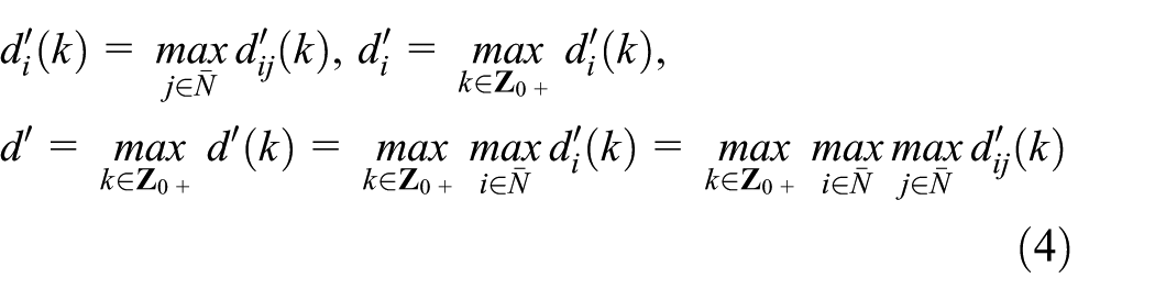
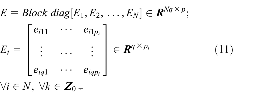
, , where , , , and are, respectively, the state, input, output, and consensus signal of the subsystem, of respective dimensions , , and , subject to and ; , and ; , where all the parameterizing matrices are uniformly bounded and of orders being compatible with the above vectors, and the various internal and external delays are
where , ; are the component-wise accounting for maximum internal (i.e. in the state) and external (i.e. in the output) delays of the subsystems at the sampling time. See De la Sen14 and Niculescu15 and some references therein for the state-space description of systems under internal and external delays. Define the whole system through the state of dimension with a control signal of dimension , output of dimension , and a consensus signal of dimension Nq. The consensus error is of dimension . The proposed idea of “consensus” described in simple wording is that the consensus signals achieve arbitrary prefixed errors between adjacent components of the consensus signal. In the background literature, this has been often particularized to the achievement of identical consensus component signals of dimension , ; (equivalently, a zero consensus error signal) at a certain discrete time (or sample) . It turns out that one of the sub-vectors is arbitrary and non-necessarily of prefixed value. Therefore, the “consensus” consists of achieving the vector conditions ; of component-wise equivalent conditions ; , .
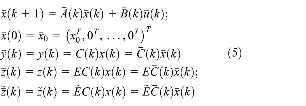
However, define for further formulation use an extended system of state of dimension , output , consensus signal of dimension , and control of dimension . The extended system together with the associated consensus signal is described as
, with and for ; , , and are of respective dimensions , , and , and
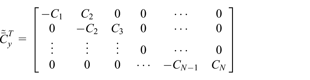
with for and for ; . The matrix with being its row; , , being such that for ; . In the same way, the matrix with being its row; , , being such that for ;
with and . Note that the particular cases of absence of internal and/or external delays can be discussed as a particular case in equations (5)–(12) being obtained from the corresponding particular case of (1). The finite-time consensus objective is defined below as the ability to fix the consensus signals of all the subsystems to have a set of arbitrarily prescribed finite mutual errors between adjacent subsystems at some finite time.
Finite-time consensus objective (FTCOA): we consider three concepts for finite-time consensus as follows:
• The interconnected system (1)–(2) achieves a (strong) finite-time consensus objective, or that it is finite-time consensus objective achievable, if there is some such that ; for any given and any given ; , under some control sequence , which can be dependent on and ; . Then, it is said that the system (1)–(2) is .
• The interconnected system (1)–(2) achieves a standard finite-time consensus objective (SFTCOA) if there is some such that ; for any given , under some control sequence , which can be dependent on . Then, it is said that the system (1)–(2) is . This is a very usual consensus objective being invoked in most of the background consensus literature in the sense that the consensus errors of all the interconnected subsystems achieve zero values, or if there is an interconnection-free system, then all its consensus signal components achieve the same values. In addition, and usually, the consensus objective is stated as an asymptotic one. See, for instance, the literature1,2,3,5,7 and references therein. However, the consensus objective stated in this article can be also and optionally a finite-time one while targeting non-zero errors between the candidate signals for the consensus achievement. So, the consensus can be stated as a finite-time or as asymptotic objective according to design requirements. A consensus vector signal is defined with ordered groups of sub-vectors being candidates to achieve the consensus. As a result, a consensus error signal, being defined as errors between the adjacent groups of sub-vectors, is targeted to reach a prefixed value (being zero or non-zero, in general) in either finite-time or asymptotically. This is the base of the proposed methodology rather than the definition of consensus protocols. Concerning the background literature, the design of linear consensus protocols and their asymptotic convergence properties have been investigated in Saber and Murray.1 In Saber et al.,2 the concept of cooperation is interpreted as giving consent to providing a state and following a common protocol that serves the group objectives. In Philip Chen et al.,5 the consensus objective is basically asymptotic and the related design is based on observers. However, the problem of designing optimal protocols, associated uniqueness and asymptotic reachability is focused on in Li et al.7 Also, an interpretation of consensus to the light of the synchronization of several coupled Kuramoto’s modeled oscillators is focused on in Strogatz.3 The synchronization objective is asymptotic in the sense that they reach common asymptotic limit cycles so the errors between their solutions are ideally targeted as zero.
• The interconnected system (1)–(2) achieves a weak finite-time consensus objective (WFTCOA) if there is some such that ; for any given and some ; , under some control sequence , which can be dependent on and ; . Then, it is said that the system (1)–(2) is , where . Note that if the system (1)–(2) is , then it is for any given (and all ).
The following result is concerned with finding explicit conditions on the consensus Gramian for the consensus achievement in finite time in the strong and weak senses. Also, the minimum number of samples for consensus achievement in the time-invariant case is related to the degree of the minimal polynomial of the matrix of dynamics of the whole system.
Theorem 1
The following properties hold:
(i) The system (1)–(2) is if and only if , where is the consensus Gramian on defined by
where and , since , are full rank sparse matrices with zero/unity entries such that and ; , where
where the effective implementable control sequence is generated by the components of below
Furthermore, it can be always found some for any given such that the system (1)–(2) is for any .
(ii) Assume that system (1)–(2) is time-invariant. Then, it is if and only if , where
is the consensus Gramian on , where ; with being the degree of the minimal polynomial of and being the controllability matrix of the pair . Equivalently, the time-invariant system (1)–(2) is if and only if . If , then this condition becomes simplified to .
(iii) If the time-invariant system (1)–(2) is , then it is for any . If it is , then it is for any arbitrary for the state got from any initial and any control on the interval . If it is not , then it is not for any .
Proof
Consider the auxiliary extended control
for some to be determined. Such a control can give repeated (then redundant) components in the presence of point external delays. Direct calculations yield
Since the consensus Gramian is positive definite, any predefined under the constraint
is achieved for any given via
through the unique control sequence
where
and such a control sequence (19) exists, depending on each given and if and only if is full rank, that is, if and only if the consensus Gramian matrix factorized as
is non-singular. The sufficiency part of Property (i) has been proved. The necessity part follows from the Rouché–Frobenius theorem from linear algebra by noting that the linear algebraic system
where and are, in general non-unique, matrices with zero and unity entries of respective full row and column ranks used to equalize the identical components of the auxiliary input vectors, with redundant repeated components, and with their independent component vectors in the identities and ; . Note that the linear algebraic system (21) has a unique solution for any given left-hand-side if and only if the matrix is full rank, that is, if and only if the consensus Gramian , then being non-singular since is full rank with at least as many columns as rows. Thus, the Gramian is full rank since it is a square matrix.
Remark in the proof
If the Gramian is rank-defective, then a singular matrix, but Rouché–Frobenius still holds (i.e. the left-hand side of equation (21) depends linearly on the columns of the Gramian), then the algebraic system is still solvable, but compatible indeterminate, and then it has infinite solutions.16 However, note that if is full rank then the Gramian is also full rank in view of its factorization as a matrix product with its transpose, both full rank and non less columns of the first one compared to the number of its rows. Thus, it is non-singular since it is a square matrix and the solution is unique.12,13 In this case, the algebraic linear system is compatible determinate and the left-hand side of (21) always depends linearly on the columns of the Gramian.
However, it turns out that, if the vector belongs to the linear span of the column vectors of the right-hand side matrix of equation (20) for any given and some existing , then Rouché–Frobenius theorem still holds leading to an indeterminate compatible linear algebraic system (20) having a (in general, non-unique) control sequence solution. Hence, it can be always found some for any given such that for any . To prove Property (ii), note that, in the time-invariant case, the minimum value for is since from Cayley–Hamilton theorem for some set of real constants dependent on each given integer , and since one then has, for any given integer , that
If , then is full row rank, and then non-singular, so that the conditions (22) are equivalent to with . Property (ii) has been proved. Property (iii) is obvious from equation (22) and the facts that, for any
and, for any
Note that is the (state) controllability matrix of the pair , is the output controllability matrix of the triple while is the consensus-error controllability matrix of the triple with respect to the auxiliary input . Theorem 1 leads directly to the two subsequent results. The first one proves the achievement of the weak finite-time consensus provided that the strong one version is achievable, the last one also implying the achievement of the standard finite-time consensus for zero consensus error signal. The second subsequent result compares finite-time consensus achievability to state/output controllability in the time-invariant case and establishes that they are, in general, different properties.
Corollary 1
If the system (1)–(2) is time-invariant, then:
(i) If it is then it is for any given .
(ii) It is if and only if it is .
Corollary 2
The following properties hold:
(i) If the system (1)–(2) is controllable and (respectively, output-controllable and for some ), it cannot be for any and conversely.
(ii) Assume that the system (1)–(2) is either controllable with ; or output-controllable with ; . Then, it is for some . The converse assertions are not true, in general.
are, respectively, the output controllability and the controllability Gramians, with respect to the input sequence . Thus, one has for any
so that a full rank of does not imply full ranks of and and conversely. Property (i) has been proved. To prove Property (ii), first assume that and ; . If the controllability Gramian is full rank so that the state can be prefixed to any value at finite time so that the consensus Gramian is full rank and the errors can be prefixed to any prefixed value; , . The converse is not necessarily true since each component has dimension so that, if the consensus Gramian is full rank, (i.e. of order ), this does not imply that the controllability Gramian is full rank (i.e. of order ). Now, assume that and ; . A close conclusion arises for respective ranks (consensus) and (output controllability) with .
Corollary 2 establishes that if controllability holds and the consensus signal is the state signal itself, then the consensus error can be fixed at any value through some control sequence in finite time. The converse is not true, in general. For instance, assume that the system is not completely controllable so that some sub-state cannot be prefixed in finite time. It still would be possible that all the remaining sub-states track that one with some non-zero or zero-error so that finite-time consensus is achievable while the system is uncontrollable. A similar reasoning can be given for output controllability if the consensus signal consists of the outputs of the subsystems. Now, rewrite the consensus Gramian of (13) as follows
where is a nominal consensus Gramian subject to a parametrical consensus error
It is of interest to characterize in terms of norms a certain tolerance to parametrical disturbances being compatible with the maintenance of the nominal consensus. It is well-known that the continuity of the eigenvalues with respect to the matrix entries implies that a non-singular matrix is still non-singular under a certain tolerated amount of additive uncertainty. Based on this principle, Banach’s Perturbation Lemma17 leads the following finite-time consensus result.
Theorem 2
Assume that the nominal consensus Gramian is positive definite, that is, . Then, the system (1)–(2) is if
The constraint (31) is guaranteed if is sufficiently small with respect to the minimal eigenvalue of such a nominal Gramian, where one has from equations (8)–(10) that
for and .
Proof
The condition (31) guarantees that equation (29) holds so that
from the continuity of all the eigenvalues with respect to all the matrix entries. To prove that equation (31) holds for a sufficiently small , first note that for any given real symmetric matrices and , then the real symmetric matrix if the constraint
holds since then . If , then equation (35) holds. Otherwise, if , then equation (31) is guaranteed under the sufficiency-type condition
The subsequent part of the proof is organized to guarantee the fulfillment of equation (36) by ensuring that the minimum eigenvalue of the nominal consensus Gramian exceeds the of the consensus Gramian error. Then, one gets from equation (13) that
where
where is Landau’s little o. Since , it follows from equation (38) that , for a small enough compared to . Then, .
Asymptotic-type consensus objectives are now defined as follows:
The standard asymptotic consensus objective (SACOA) is formulated as the achievement of the property as ; for any given , under some control sequence which can be dependent on . Then, it is said that the system (1)–(2) is , that is, standard asymptotic consensus objective achievable.
The trivial standard asymptotic consensus objective (TSACOA) is defined for the particular case of the system (1)–(2) being with as ; . Note that this asymptotic objective is directly fulfilled, in a sufficiency-type context, for any consensus signal of dimension not exceeding that of the state and defined by some linear transformation from the output (or the state) while it becomes independent of the control, output, and consensus error matrices (and then independently of the definition of the consensus signal) if the unforced system (1) is globally asymptotically stable. See, for instance, the literature11,18,19 and references therein. Thus, it turns out that asymptotic consensus objectives can merit some attention only in cases when asymptotic stability fails.
The asymptotic consensus Gramian is defined by taking the limit as , provided that such a limit exists, as follows
Asymptotic consensus objectives are now formulated based on the above consensus Gramian.
Theorem 3
Assume that the asymptotic consensus Gramian exists. Then, the following properties hold:
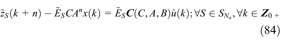
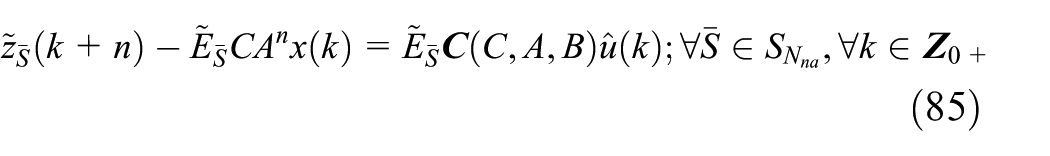
(i) The system (1)–(2) is if
(ii) The system (1)–(2) is if for some .
Assume, in addition, that
or, in particular, that
Then
(iii) If the system (1)–(2) is for some finite and ; for some finite non-negative integer , then it is .
Proof
Property (i) follows from the definition of the limit defining asymptotic consensus Gramian (39) which is, furthermore, positive definite and then finite. Property (ii) follows since the given condition implies that the system (1) is globally asymptotically stable. Property (iii) is obvious since, by construction
and the minimum eigenvalue of is positive from equation (40), and
Since and the sequences and are bounded, then the maximum eigenvalue of is bounded from equation (41). Thus, all the eigenvalues of are positive and uniformly bounded for any integer . Furthermore, since is positive definite for all since the system (1)–(2) is , then, from the assumption of Property (iii), the consensus Gramian superior and inferior limits as are finite so the limit exists, and it is positive definite.
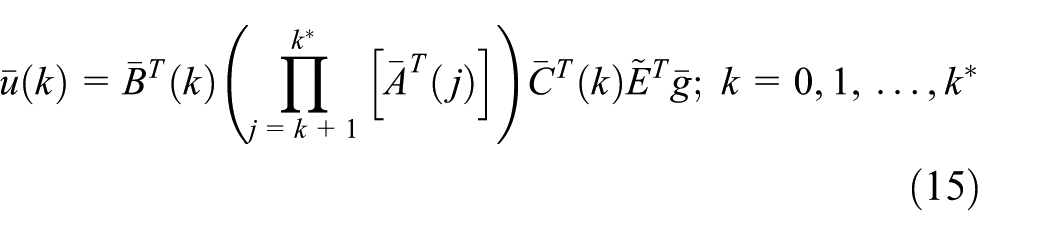
The control sequence defined from (19) as
is valid to achieve the standard asymptotic consensus objective.
Note that the global asymptotic stability of the system is not necessary for Theorem 3 to hold since the asymptotic consensus Gramian can exist even if is unbounded and does not vanish as . It is easy to see that two variables fulfilling the asymptotic consensus objective can both diverge with identical sign while its mutual error converges asymptotically to zero. This is not the case for the standard asymptotic stability. For instance, if equation (39) is evaluated with and being identity matrices of the same order so that the Gramian is associated with the whole state, its positive definiteness would require, as expected, that as , that is, that the system matrix is convergent so that the unforced system is globally asymptotically stable.
Alternative consensus tests in the time-invariant case
In the time-invariant case, it is possible to derive “ad-hoc” spectral tests for finite-time consensus. To discuss if the system (1)–(2) is , we can extend the Popov–Belevitch–Hautus controllability eigenvalue test12,13 as follows. Take time-derivatives in equation (5) in the time-invariant case and then take Z-transforms so that one gets
where is the Z-transform argument, being formally equivalent to the one-step discrete advance operator, and the superscript “hat” denotes the Z-transforms of their un-superscripted signal counterparts. Note that the generic rank (i.e. the maximum rank) of for is , even if the system is not controllable, that is, this matrix can be (eventually) rank-defective for being an eigenvalue of and then
, provided that . If the left-hand-side rank equalizes the generic rank, then there is always a solution to equation (44) for each given initial condition. Thus, the following result follows from equations (44) and (45) related to consensus of time-invariant systems based on Popov–Belevitch–Hautus spectral tests
Theorem 4
Assume that the system (1)–(2) is time-invariant. Then, the system is for if and only if:
(i) Eigenvalue test
for which a necessary condition is that provided that and are full row rank (see Theorem 1 (i)).
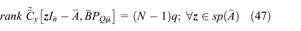
If , then the above property is guaranteed under output-controllability while it holds if and only if
where and
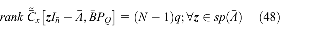
If , then the above property is guaranteed under controllability while it holds if and only if
where and ; and has a close form to that of by replacing the by identity matrices of appropriate orders, where:
(ii) Eigenvector test: assume that is the set of left-eigenvectors of . Then, the system is if and only if is not orthogonal to ; . If , then the property holds if and only if is not orthogonal to . If , then the property holds if and only if is not orthogonal to ; .
Note that the above tests are performed to give necessary and sufficient conditions for fixing the consensus error (rather than the consensus signal) to arbitrary prefixed values. Similar test on the consensus signal yield just sufficiency-type conditions with the replacement . Such tests can be easily extended to the asymptotic consensus objectives in the time-invariant cases by just considering the critically stable and unstable eigenvalues. Define . Then, the following result follows from Theorem 4
Corollary 3
Assume that the system (1)–(2) is time-invariant. Then, the system is under the eigenvalue (respectively, eigenvector) tests of Theorem 4 by checking them only for the subset of (respectively, for their corresponding eigenvectors).
Remark 1
Note that the above Corollary is applicable to the . Note also that the other two consensus objectives of section “Problem formulation” for finite time have not precise sense in the asymptotic context under the eigenvalue/eigenvector tests as time tends to infinity since the achievement of such objectives to non-zero consensus errors in infinity time depend on the whole spectrum and not only on the critically stable and unstable modes.
Consensus under feedback: some extensions to time-interval consensus and positive systems
Consider a feedback system subject to internal and external delays and linear output feedback
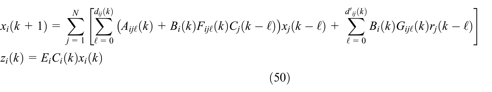
control agents for controlling an interconnected tandem of subsystems; , , , , and are, respectively, the state, control input, measured output, consensus signal, and reference signal of the subsystem for subject to , ; and ; , where and are, respectively, the internal and external delays of the subsystem at the sampling instant. All the parameterizing matrix functions are of sizes being compatible with the above vectors. The closed-loop description is
. Define a whole system through the state of dimension and an external reference signal of dimension , with maximum finite delays , ; and and . Define also an extended system of state of dimension , output , consensus signal , and reference signal of dimension . Then, one gets under zero initial conditions
, with initial conditions , and the consensus error is
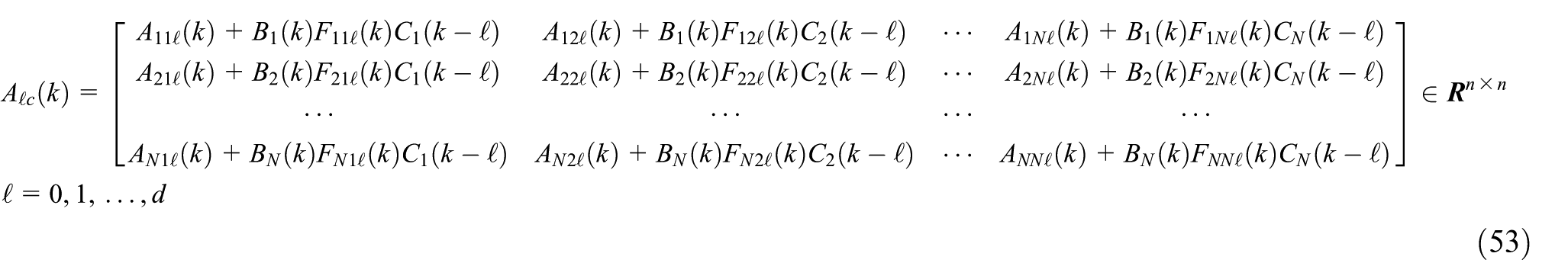
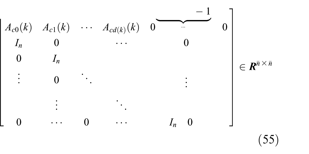
, with and for , , , and are of respective dimensions , and , and
Remark 2
If the state vector is available for measurement and state linear feedback is used instead of output feedback, then the above closed-loop description remains valid by deleting the output matrices in equations (50) and (53).
Remark 3
The results of the above sections remain valid under the parameterization replacements in equations (6), (7), (8), and (9) by those of equations (53), (54), (55), and (56), respectively, and the control (18)–(19) being accordingly modified with the new parameterization and the control being replaced with while keeping the same structure. Note that the use of the internal linear feedback does not allow the achievement of the positive definiteness of the modified consensus Gramian in the case that the one for the control does not fulfill such a property.
It is of interest to characterize the situation when a consensus is got over a set of consecutive samples with the consensus error being not necessarily zero, or even identical, for all the samples. Based on Theorem 1, we can now extend it for its validity over a set of consecutive samples. We limit the description for Theorem 1 (i).
Theorem 5
Assume the system (1)–(2) with
and let the consensus Gramian on for be
where
and define also
. Then, the system (1)–(2) is ; for some given if and only if is full row rank.
Proof
Define
where
with
Thus, if is full row rank, and since it has no less rows than columns, a necessary condition being , then has a unique solution for any given initial conditions and set of consensus error vectors .
It is also interesting to characterize the consensus objectives in the case of positive systems, that is, those which have non-negative values of the state and output components for all time under non-negative components of the initial conditions and controls.14,20 It is well-known that a linear discrete system is positive if all its parameterizing matrices (i.e. the matrix of dynamics or system’s matrix, control matrix, and output matrices) are non-negative. Also, a positive monomial matrix (then being non-singular since it has just a positive entry per row and per column) has a positive inverse and conversely. Due to the positivity-type constrains on the parameterization, the consensus errors and signals cannot be fixed arbitrarily irrespective of the initial conditions and consensus errors while keeping the positivity of the controls. In particular, for fixed initial conditions, the consensus errors are not arbitrary but they are subject to certain constraints. Therefore, the strong consensus objective as stated in Section 2 is not compatible with the positivity. A consequence of such a fact and Theorem 1 for positive systems is the following result:
Theorem 6
Assume that the system (1)–(2) is positive and its consensus Gramian on fulfills . Then, the following properties hold the following:
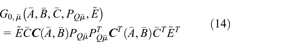
(i) The system (1)–(2) is for any given initial condition and any consensus signal vector satisfying if and only if the consensus Gramian (i.e. that defined with respect to the consensus z-output with ) is positive and monomial, where
(ii) Define, equivalently, the Gramian of (63) by its entries as
where
, where and are, respectively, the to the matrices and all of them being non-negative. Thus, a necessary and sufficient condition for Property (i) to hold is the existence of a set of non-necessarily disjoint nonempty subsets of ; such that the subsequent set of scalar conditions hold for all and
that is, is similar to except by the replacement , that is, the consensus error signal is replaced by the consensus signal to construct the respective controllability Gramian. However, note from equations (13), (15), (18), and (19) that a replacement can be performed on the control expression (19) achieving the consensus objective by replacing: (1) , and (2) . A unique control law being very close to equation (19), which achieves a weak consensus objective satisfying for any given is
Since , by hypothesis, and such a Gramian is monomial then its inverse is also monomial and positive. Since all the matrices which parameterize (1)–(2) are positive, then (1)–(2) is positive, while and , the weak consensus objective is achieved at time . The proof of Property (i) is complete. To prove Property (ii), one gets from (64) that
since
Note that is positive monomial (then also non-singular), so that its inverse exists being positive and monomial as well, if
which holds if Property (ii) holds. Note that, if is full row rank, then
Therefore, the hypotheses of Theorem 6 can be simplified and reformulated in a simpler way as follows.
Corollary 4
Assume that the system (1)–(2) is positive, is full row rank and is positive, positive definite, and monomial. Then, the system (1)–(2) is for any given initial condition and any consensus signal vector satisfying .
Examples
Example 1: consensus objective under centralized control
Consider an interconnected discrete linear and time-invariant delay-free dynamic system with subsystems with state, output, consensus, and input sequences , , , and , whose elements have respective dimensions , and , with ; and parameterizing matrices (system matrix), (control matrix), (output matrix), output-consensus matrix, and error consensus matrix. The consensus error signal, whose components are the errors between two adjacent consensus signals, is defined by the sequence .The system is subject to time-varying linear output feedback with gain sequence . One gets the following description
where is the controllability matrix of the pair and ; is generated via linear output feedback for , that is
from equation (73), where is the observability matrix of the pair , and
provided that the controller gain matrix is chosen such that the inverse in the right-hand side of equation (78) exists, where is the output-controllability matrix of the triple . If, in addition, is non-singular, then so that equation (79) can be rewritten as
, where denotes the Kronecker product of two matrices, that is, ; and denotes the vectorization of the matrix , that is, a vector with the entries of ordered by the order of its rows and the entry of each row. Note that the number of unknowns to solve (80) is since , ; , and the number of data in the left-hand side of equation (80) is since , . We get the following conclusions in view of equations (73) and (80):
If , then for any given , the system is through some control sequence ; and a necessary condition is that be full row rank. So, all other weaker consensus objectives are also achievable. The consensus objectives are also achievable if is output controllable and the consensus signal is the output or if is controllable and the consensus signal is the state. However, the two last conditions are not necessary, in general. These considerations agree with Theorems 1 and 4 for the delay-free case.
Assume that . The system is not for and any consensus error , for instance, if and under output linear feedback control (75). It is if under a zero control sequence. It is also for any and output linear feedback control for some sequence of controller gains if is full row rank and the system is observable. Note that if and the system is observable since is full row rank, which equalizes that of , which is also full, and can be chosen for any given so that be linearly dependent on the columns of so that the linear algebraic system (80) is compatible determinate (if provided that the obtained is non-singular, then have to be also non-singular for ) or compatible indeterminate (if ) in the unknown vector solution . After computing any such solution can be obtained since is known. If and is chosen so that
Then, the weak consensus objective is also achievable for some existing controller gains, but the objective is redundant in the sense that the consensus objective could be redefined by deleting some of the consensus signal components. If is eventually singular while is non-singular, then equation (79) is rewritten as
where can be uniquely calculated from each solution to equation (81) provided that at least one solution exists for . Thus
has at least a solution if
3. In the presence of state discrete delays, the problem can be solved in a similar way using the augmented system which includes in its state the necessary number of consecutive delayed states.
Example 2: consensus objective under decentralized or partially decentralized control
Decentralized control is a powerful tool for the case when the feedback information is too exhaustive to be handled simultaneously by multiple control agents.21 More recent related discussions are given in Mahmoud22 for decentralized delay-dependent stability and stabilization methods and in Mahmoud23 for decentralized reliable control under control failures. Also, a wide and general framework for decentralized control of large-scale systems is provided in Mahmoud.24 Note that Example 1 uses, in general, centralized linear output feedback control of the form ; in the sense that each subsystem controller has the feedback information of the output of the whole interconnected system. It can happen that the consensus objective is achievable under decentralized control of the form for , (i.e. each subsystem has a local controller based on measurements on its own output or, in other words, the whole output feedback gain matrix is block diagonal for all samples21). Finally, it can happen that the consensus objective, supposed to be achievable under centralized control, is not achievable under decentralized control while it can be achieved under partly decentralized control. This control action refers to the fact that at least one subsystem needs information from the outputs of other subsystems while at least one of such subsystem needs only feedback from its own output. In this case, the whole output feedback gain matrix is either lower-triangular or upper-triangular. Under decentralized or partially decentralized control, the control effort becomes cheaper related to the centralized case since the global output information is not supplied to all the local controllers (which are in certain applications allocated in different locations, and may be, at long mutual distances, for example, in tandems of hydroelectric power stations along a river).
Now, assume Example 1 with ; with and and define , such that and , and assume that . Thus, is the (non-necessarily unique) number of subsystems for which the consensus is achievable and is the (non-necessarily unique) number of subsystems for which the consensus objective is not achievable. If the consensus is achievable for the whole set of the interconnected subsystems , then . Note that . Since the consensus is not achievable for the whole set of subsystems, but only for some non-necessarily unique subset of them, it is possible to use linear output feedback on the non-consensus subsets to try to increase the admissible cardinals of the consensus sets from to some integer . Note that there are combinations of interconnected subsystems each of cardinal for which the consensus is directly achievable (the ideal case being when is unity, that is, with ) and combinations of subsystems of cardinal for which the consensus is not directly achievable. Thus, let and be, respectively, the sets of all combinations of subsystems for which consensus is achievable or non-achievable. The proper subset of combinations of all the existing subsets has cardinal if consensus is achievable for all of such subsets. Otherwise, we have the set of subsets of respective cardinal of the interconnected system where the consensus is achievable
and the set of subsets of respective cardinal of the interconnected system where the consensus is not achievable
Note that the matrices and for and, respectively, for , are obtained directly from , and , , ; , and ; . Then, we consider the system (72)–(73) with (73) being split into two parts as follows
And, we perform three steps:
Step 1. Check if consensus if possible under decentralized control, that is, under a block diagonal controller gain, in particular, by resolving Example 1 through a block diagonal controller matrix. In the case of the objective failure, it is possible to check for partially decentralized control by first checking the consensus achievability of the system with the set of tentative control laws with as many subsystems as possible under decentralized local control. This gives (at least) a maximum subset of subsystems of the whole set .
Then, check, in a second step, if at least one of such feedback laws under partial decentralized control combined with centralized control for the remaining subsystems leads to consensus achievability.
Step 2. Use (partially) centralized linear output feedback only on the subsystems where the consensus is not primarily achievable under decentralized control, that is
for each for a set of gains , for , with being the set of admissible parameterizations of the controller gains.
Step 3. We check , where the “bar” superscripts define the corresponding matrices or controller domains by completing with appropriate zero matrix blocks those which are not affected by control feedback since are referred to . If , then the injected partial linear output feedback has improved the consensus achievement between the various subsystems. If , then the consensus objective achievement is not improved via partial linear output feedback.
Example 3: consensus objective in a set of network oscillators
Consider a simple network of second-order oscillators with linear interconnections. Each individual oscillator can be modeled as a pendulum clock and such a model can be linearized as
for small angular displacements around the equilibrium point , where denotes the natural frequency of the ith oscillator, which is subject to a forcing term defined as
Such a forcing term consists of an external input and an additional feedback term that couples the position state from other pendula. The coefficients denote the coupling strength between oscillators i and j. It is assumed that each clock is not coupled to itself so ; and the couplings between oscillators i and j are reciprocal so ; with .
The system of coupled oscillators can be represented in state variables form by defining the state vector of each oscillator as , . Such a model is given by
where , , and are, respectively, the input, output, and state vectors of the system. The matrices of this system representation are , , and , where each block is given by
with . Note that the components of the output vector are the angular positions of each individual oscillator in this system representation.
In particular, a network with oscillators is considered. The natural frequencies of such oscillators are, respectively, , , , and while the coupling strength between oscillators is given by the matrix
where . The zeros in the diagonal of indicate that each oscillator is not coupled to itself. The entry ; with is the coupling strength between the oscillators i and j. Also, such a coupling matrix indicates that each oscillator is coupled to its nearest neighbor with the maximum coupling magnitude and the coupling magnitude decreases exponentially with the relative distance between oscillators. In this context, the coupling strength between the oscillators i and j, , would be , where denotes the relative distance between such oscillators.
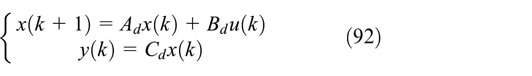
The continuous-time model (89)–(91) is discretized using a zero-order hold (ZOH) with a sampling period in order to illustrate some of the consensus results described in the previous sections of this article. In this way, a discrete model given by
where , , and denotes the state, input, and output at the kth sampling instant , and the matrices , , and of the discrete representation of the system are related to those of the continuous-time one by means of
The consensus signals are chosen as the angular positions of the individual oscillators so and , where denotes the forth-order identity matrix. Then, the consensus error vector is , so the matrix is given by
By direct calculations from equation (92), it follows that the evolution of consensus error vector is given by
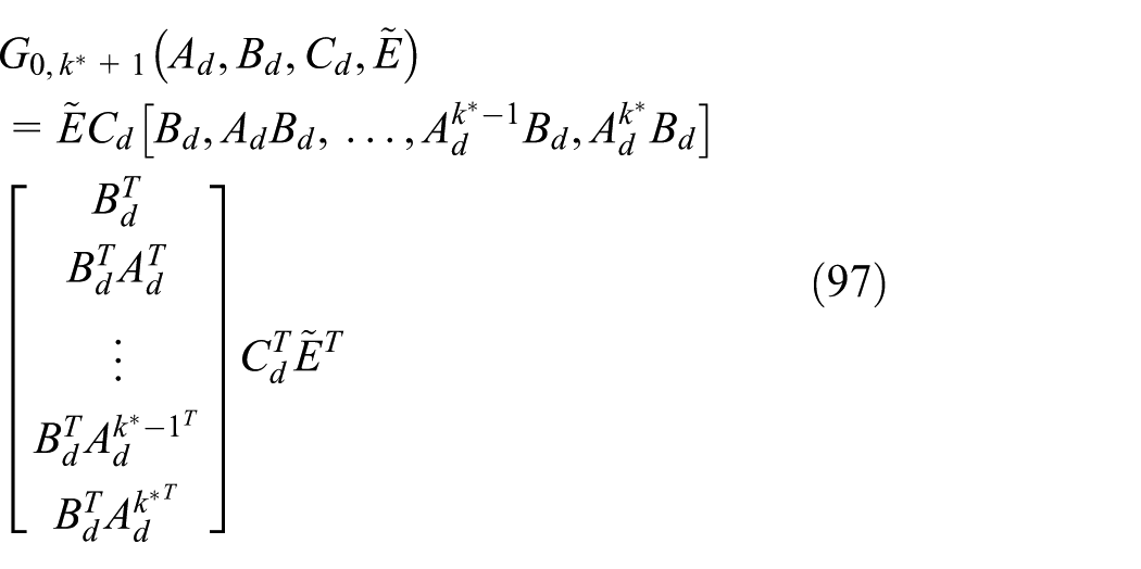
under the application of an input vector whose values at each sampling instant, from to , are grouped as
where , , and is the consensus Gramian defined as
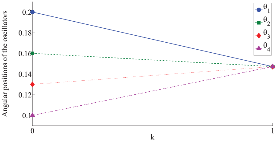
The standard finite-time consensus objective of the system for an arbitrary initial condition at a given sampling instant , with , is achievable under a control sequence defined as (96) with
if the Gramian is not singular, that is, invertible. In particular, if the initial condition is , that is, ; and , , , and , and the control vector leads the system to the standard consensus at the sampling instant as it can be seen in Figure 1. Note that the angular positions of the four individual oscillators concur at such a consensus sampling time instant.
Evolution of the angular positions of the oscillators from the initial instant to the consensus instant .
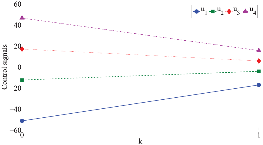
The control vector sequence with and leads the system to the standard consensus at the sampling instant from the same initial condition if as it is shown in Figure 2. The evolution of the control signals to achieve such a consensus is displayed in Figure 3.
Evolution of the angular positions of the oscillators from the initial instant to the consensus instant .
Evolution of the control signals to achieve the consensus at the instant .
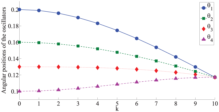
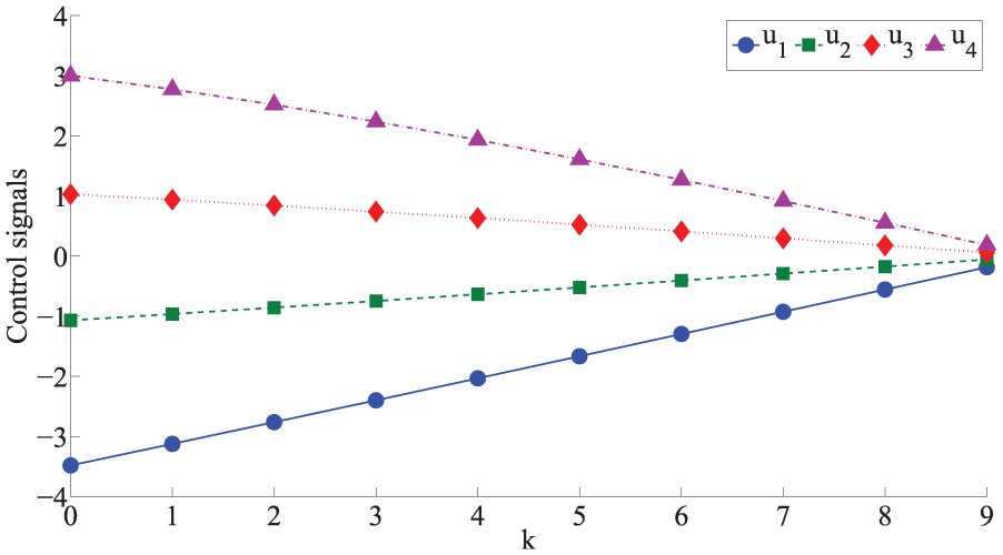
In the same conditions, if one desires to achieve the consensus at the instant (i.e. if ), then the evolution of the angular positions and control signals are, respectively, displayed in Figures 4 and 5.
Evolution of the angular positions of the oscillators from the initial instant to the consensus instant .
Evolution of the control signals to achieve the consensus at the instant .
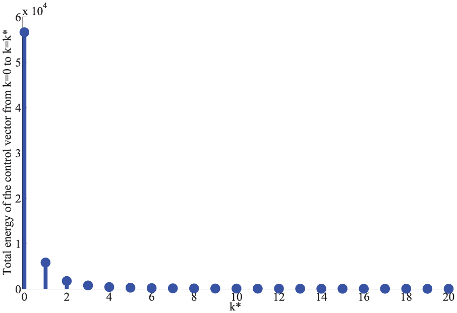
One can see that the amplitude of the control signals is large when one requires the consensus objective to be achieved fast, that is, in a little number of sampling instants. In this sense, one can define a cost function to measure the average of the control effort per sampling instant to achieve the consensus objective as follows
where is the energy of the signal from the initial sampling time to the sampling time . In this context, Figures 6 and 7 display the total energy of the control signals, that is, , to lead the angular positions of the oscillators from their initial positions to a consensus position at the instant for different values of . Figure 7 shows a more detailed information for values of larger than 3. Figures 8 and 9 display the average energy of the control signals per sampling time to lead the angular positions of the oscillators from their initial positions to a consensus position at the instant for different values of , that is, . Figure 9 shows a more detailed information for values of larger than 3. Finally, Figures 10 and 11 display the maximum energy of the control signals at the sampling time instants from the initial time to the consensus time at the instant for different values of . Figure 11 shows a more detailed information for values of larger than 3. Note that such a maximum value is always taken at the initial sampling instant. Also, note that the required energy, the average energy and the maximum value of the energy of the control signals at the sampling instants to lead the system from the initial condition to the consensus state decrease as the consensus time instant increases. Moreover, such quality measures about the control signals converge as the value of the consensus time instant goes to infinity. As a consequence, a trade-off between the energy of the control input signals and the speed of the system to achieve the consensus can be taking into account to choose the instant for the consensus. For instance, a value can be appropriate in the example of the four oscillators since the consensus is achieved in a sufficiently short time interval while the control energy required for such a purpose is small enough. Furthermore, the faster the consensus is targeted, the smaller computational effort is needed while, however, the needed control energy increases. In other words, if the consensus is targeted for larger time intervals, then the necessary control energy consumption is usually smaller compared to the case when the same objective is tried on smaller time intervals.
Total energy of the control signals to achieve the consensus at the instant .
Total energy of the control signals to achieve the consensus at the instant .
Average energy of the control signals per sampling instant to achieve the consensus at the instant .
Average energy of the control signals per sampling instant to achieve the consensus at the instant .
Maximum of energy of the control signals from the initial sampling instant to achieve the consensus at the instant .
Maximum of energy of the control signals from the initial sampling instant to achieve the consensus at the instant .
Conclusion
This article has dealt with the conditions for consensus under appropriate controls in linear interconnected discrete systems with, in general, multiple internal and external, in general, incommensurate delays. The consensus signals can be defined as being distinct of the output/state components of the interconnected subsystems and can be linear combinations of some of such components. The formulation and discussion of the consensus objectives are stated using algebraic tools. It has not being assumed, in the most general context, that the initial conditions and/or the consensus error are prefixed to zero and that this is necessarily an asymptotic objective. In this way, the consensus errors for the various adjacent subsystems can be distinct, in general, for purposes of generalization of the concept of consensus. The control sequences leading to the achievement of the consensus objectives are characterized explicitly via a so-called consensus Gramian. The various given consensus objectives, which have been defined in this article, are related to their achievability either at finite time, that is, for a finite set of discrete samples, or asymptotically. A further extension is given to formulate the consensus of positive systems which implies some extra restrictions on the consensus Gramian, in particular, that it be monomial. Finally, some worked examples have been presented and discussed.
Footnotes
Acknowledgements
The authors are also very grateful to the referees by their interesting suggestions.
Handling Editor: Jose Ramon Serrano
Declaration of conflicting interests
The author(s) declared no potential conflicts of interest with respect to the research, authorship, and/or publication of this article.
Funding
The author(s) disclosed receipt of the following financial support for the research, authorship, and/or publication of this article: The authors are very grateful to the Spanish Government and European Fund of Regional Development FEDER for Grant DPI2015-64766-R and to the UPV/EHU by its support via Grant PGC 17/33.
ORCID iD
Manuel De la Sen
Santiago Alonso-Quesada
References
1.
SaberROMurrayRM. Consensus protocols for networks of dynamic agents. In: Proceedings of the 2003 American control conference, vols. 1–6, Denver, CO, 4–6 June 2003, pp.951–956. New York: IEEE.
2.
SaberROFaxJAMurrayRM. Consensus and cooperation in networked multi-agent systems. Proc IEEE2007; 95: 215–233.
3.
StrogatzSH. From Kuramoto to Crawford: exploring the onset of synchronization in populations of coupled oscillators. Physica D2000; 143: 1–20.
4.
BasarTEtesamiSROlshevskyA. Convergence time and quantized metropolis consensus over time-varying networks. IEEE T Automat Contr2016; 61: 4048–4054.
5.
Philip ChenCLWenGXLiuYJ. Observer-based adaptive backstepping consensus tracking control for high order nonlinear semi-strict-feedback multiagent system. IEEE T Cybernetics2016; 46: 1591–1601.
6.
BausoDGiarreLPesentiR. Non-linear protocols for optimal distributed consensus in networks of dynamic agents. Syst Control Lett2006; 55: 918–928.
7.
LiYVoosHDarouachM. Nonlinear protocols for distributed consensus in directed networks of dynamic agents. J Frankl Inst2015; 352: 3645–3669.
8.
ZhuWLiWZhouP. Consensus of fractional-order multi-agent systems with linear systems via observer-type protocol. Neurocomputing2017; 230: 60–65.
9.
YangCLiWZhuW. Consensus analysis of fractional-order multi-agent systems with double-integrator. Discrete Dyn Nat Soc2017; 2017: 9256532.
10.
ZhuWChenBYangJ. Consensus of fractional-order multi-agent systems with input timed delay. Fract Calc Appl Anal2017; 20: 52–70.
11.
HanFFengGWangY. A novel dropout compensation scheme for control of networked T-S fuzzy dynamic systems. Fuzzy Set Syst2015; 235: 44–61.
12.
KailathT. Linear systems. New Jersey: Prentice-Hall, 1980.
13.
IonescuVOaraCWeissM. Generalized Riccati theory and robust control. A Popov function approach. Chichester: John Wiley & Sons, 1999.
14.
De laSen M. On positive stability of a class of time-delay systems. Nonlinear Anal: Real2007; 8: 749–768.
15.
NiculescuSI. Delay effects on stability. A robust control approach (LNCIS Lecture Notes in Control and Information Sciences No. 269). Berlin: Springer, 2001.
16.
WatkinsDS. The matrix eigenvalue problem. GR and Krylov subspace methods. Pennsylvania: SIAM, 2007.
17.
OrtegaJM. Numerical analysis. New York: Academic Press, 1972.
18.
DelasenM. Online optimization of the free parameters in discrete adaptive-control systems. IEE P: Contr Theor Ap1984; 131: 146–157.
19.
Bilbao-GuillernaADelaSenMIbeasA. Robustly stable multiestimation scheme for adaptive control and identification with model reduction issues. Discrete Dyn Nat Soc2005; 2005: 31–67.
20.
DelasenM. Preserving positive realness through discretization. Positivity2002; 6: 31–45.
21.
SinghMG. Decentralized control, systems and control series. Amsterdam: 1981.
22.
MahmoudMS. Decentralized stabilization of interconnected systems with time-varying delays. IEEE T Automat Contr2009; 54: 2663–2668.
23.
MahmoudMS. Decentralized reliable controls of interconnected systems with time-varying delays. J Optimiz Theory App2009; 143: 497–518.
24.
MahmoudMS. Decentralized systems with design constraints. London: Springer-Verlag, 2011.