Sage Journals: Discover world-class research

Abstract

Supercritical water fluidized bed is a promising reactor which can realize the efficient and clean gasification of coal to produce hydrogen. As the high pressure and temperature inside supercritical water fluidized bed, the study of the detail flow behaviors needs the help of numerical method. Considering the limitation of the two-fluid method and discrete element method, the computational particle fluid dynamics method was applied to this work. When particle size distribution was taken into consideration, the simulated results showed that the transformation from fixed bed regime to fluidized bed regime is a gradual process. With the increase in superficial fluid velocity, particles in small diameter migrate to the top of the bed and there exits layering phenomenon in the bed. Besides, though the particles are categorized as Geldart B group, the minimum fluidization velocity is not equal to the minimum bubbling fluidization velocity and there is a complicated bed expansion process after incipient fluidization. The bed expansion process is also influenced by the particle size distribution.

Keywords

Supercritical water fluidized bed computational particle fluid dynamics method particle size distribution Geldart B

Introduction

With the environmental pollution and energy shortage problems becoming increasingly serious, hydrogen, an ideal energy carrier, has gained more and more attention. Supercritical water (SCW) gasification technology has been proved that it is a promising approach for conversing coal and wet-biomass into hydrogen efficiently and cleanly.^1,2 Supercritical water fluidized bed (SCWFB) is a new-type reactor which can avoid plugging and slagging problems often taking place in tubular reactor and improve the gasification efficiency. The concept of SCWFB was first proposed by Matsumura and Minowa.³ Lu et al.⁴ successfully developed the first SCWFB reactor for the gasification of biomass. Jin et al.⁵ further improved the reactor for the efficient gasification of high concentration coal slurry with long continuous time. But there are still not enough theories for the design of SCWFB. So far, little work has been done for the study of fluidizing bed operating at high temperature and pressure. Liu et al.⁶ studied the supercritical CO₂ fluidized beds, in which the granular materials belonging to Geldart groups A, B, and C and proposed a criterion to determine the fluidized regime. Vogt et al.⁷ carried out a comprehensive experimental investigation to study the fluidization behavior with supercritical CO₂ at pressure up to 30 MPa for Geldart A and B powders. Potic et al.⁸ introduced a SCW micro-fluidized bed to study the correlations for homogeneous bed expansion and minimum bubbling velocity for process conditions up to 773 K and 244 bar. Lu et al.⁹ did a series of experiments to study the hydrodynamics of SCWFB within the range of 633–693 K and 23–27 MPa, evidencing that Ergun’s equation is applicable for SCWFB and deriving the empirical equation for the minimum fluidization velocity. But the details of particle distribution and fluid hydrodynamics characteristics remain unclear. As a result, there are some key problems which cannot be solved for the lack of in-depth study.⁹ Thanks to the development of computer technology, numerical simulation can be an effective way to study the complex solid–fluid flow behaviors inside SCWFB, which is necessary for the design, scaling up, and operating condition optimization of the reactor.

Recently, there are two major numerical methods applied to particle fluid flow simulation: the Euler–Euler method and the Euler–Lagrange method. In Euler–Euler two-fluid model (TFM), both particle phase and fluid phase are treated as interpenetrating continuous medium, and the conversation equations are derived and correlated via constitutive relationships that obtained from empirical formula and kinetic theory.¹⁰ TFM has the advantages of high calculation speed and wide applicable rang. However, there are many controversies for the assumption of treating the particle phase as continuous medium.¹¹ In Euler–Lagrange method, one is discrete element method (DEM),¹² in which the particle phase is treated as discrete phase and individual particle motion is obtained by solving Newton’s second law. Forces caused by collision of particles are taken into account, making the model more precise for the simulation of granular flow. DEM has a high accuracy, and it is easy to generate detailed particle-scale information, which is important to elucidate the mechanism of complicated particle fluid flow behavior. Unfortunately, DEM is limited in applicability for the complex dense particle–particle interaction calculations when a large number of particles involved. It is usually restricted to the two-dimensional (2D) simulations.¹³

To compensate the limitation of TFM and DEM, the computational particle fluid dynamics (CPFD) method has been developed in recent years. CPFD method models fluid phase as continuum with strong coupling with the discrete particles. The particle phase is modeled as discrete phase following the multiphase-particle-in-cell (MP-PIC) numerical method from Andrews and O’Rourke¹⁴ and Snider et al.,¹⁵ which is a Lagrangian description of particle motion via ordinary differential equations with coupling with the fluid. Compared to DEM, CPFD method eliminates the difficulties associated with calculating inter-particle interactions for dense particle flows with high volume fractions by the normal stress model, which is robust and can eliminate the need for an implicit calculation of the particle normal stress on the grid. A concept of computational particle is also defined where particles with the same properties (species, size, density, etc.) are grouped. The computational particle is a numerical approximation which reduces the simulation costs for an industrial-scale simulation containing huge number of particles. In recent years, CPFD method has been successfully applied to studying fundamental granular flow characteristics,^16,17 and these works validated the accuracy and reliability of CPFD method in turn.

In this article, CPFD method was used to investigate the fluidization characteristics in SCWFB with consideration of particle size distribution in three dimensions. The simulation results were compared to concerned experimental and numerical results published in the literature.^18,19

Numerical method

In CPFD method, the equations of fluid phase are derived from the kinetic theory for dilute gases or continuum points of view. The volume averaged fluid mass and momentum equations²⁰ are

\frac{\partial ε_{f} ρ_{f}}{\partial t} + \nabla \cdot ε_{f} ρ_{f} u_{f} = 0

(1)

\frac{\partial ε_{f} ρ_{f} u_{f}}{\partial t} + \nabla \cdot ε_{f} ρ_{f} u_{f} u_{f} = - \nabla p - F + ε_{f} ρ_{f} g + \nabla \cdot ε_{f} τ_{f}

(2)

where ε_f is the fluid volume fraction, ρ_f is the fluid density, u_f is the fluid velocity, p is the fluid pressure, g is the gravitational acceleration, and τ_f is the fluid stress tensor. F is the rate of momentum exchange per volume between the fluid and particles phases which is given below. The particle phase is modeled by the Lagrangian method following Newton’s second law. The particle acceleration is

\frac{d u_{p}}{dt} = D_{p} (u_{f} - u_{p}) - \frac{1}{ρ_{p}} \nabla p + g - \frac{1}{ε_{p} ρ_{p}} \nabla τ_{p}

(3)

where u_p is the particle velocity, D_p is the drag coefficient at the particle location, ρ_p is the particle density, and τ_p is the particle normal stress. ε_p is the particle volume fraction, and from conservation of volume, the sum of fluid and particle volume fractions equals unity, ε_p +ε_f = 1. The terms in the right side represent acceleration due to aerodynamic drag, pressure gradient, gravity, and gradient in the inter-particle normal stress, respectively.

Particle properties are mapped from the Eulerian grid to particle locations. Particle properties are also then mapped from particles to the grid to get grid-based properties, such as the particle volume fraction at cell ξ

ε_{p ξ} = \frac{1}{V_{ξ}} \sum_{1}^{N_{p}} V_{p} n_{p} S_{p ξ}

(4)

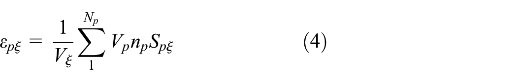
where V_ξ is the volume of cell ξ, V_p is particle volume, n_p is the number of particles in a computational particle, S_pξ is the interpolation operator, and the summation is overall computational particle N_p. The implicit numerical integration of the particle velocity equation is given by

u_{p}^{n + 1} = \frac{u_{p}^{n} + Δ t [D_{p} u_{f, p}^{n + 1} - \frac{1}{ρ_{p}} \nabla p_{p}^{n + 1} - \frac{1}{ρ_{p} ε_{p}} \nabla τ_{p}^{n + 1} - g]}{1 + Δ t D_{p}}

(5)

where $u_{p}^{n + 1}$ is the interpolated fluid velocity at the particle location, $\nabla p_{p}^{n + 1}$ is the interpolated pressure gradient at the particle location, and $\nabla τ_{p}^{n + 1}$ is the interpolated particle stress gradient at the particle location. The particle movement is given by

\frac{d x_{p}}{dt} = u_{p}

(6)

The new particle location at the next time step is then

x_{p}^{n + 1} = x_{p}^{n} + u_{p}^{n + 1} Δ t

(7)

The fluid momentum equation implicitly couples fluids and particles through the inter-phase momentum transfer. The inter-phase momentum transfer at momentum cell ξ is

F_{ξ}^{n + 1} = \frac{1}{V_{ξ}} \sum_{p} S_{ξ} [D_{p} (u_{f, p}^{n + 1} - u_{p}^{n + 1}) - \frac{1}{ρ_{p}} \nabla p_{p}^{n + 1}] n_{p} m_{p}

(8)

The inter-phase drag function D_p is calculated using a drag model. Numerous literature about the empirical drag models for calculating D_p have been published. In Lu et al.’s⁹ previous investigation, it was evidenced that the Ergun model is found applicable in SCWFB through a fixed bed. With the consideration of particle sphericity, the Ergun equation is not appropriate for the void fraction larger than 0.8;²¹ when the void fraction was less than 0.8, Ergun equation was used. When the void fraction was larger than 0.8, a modified equation of the fluid resistance for a single particle can be selected. Based on many individual experimental results, Chhabra et al.²² found that Ganser’s equation is the most accurate model for predicating the drag coefficients of single non-sphere particles. So, the drag model used in this article was addressed as follows

\begin{array}{l} D_{p} = {\begin{cases} \frac{3}{4} C_{d} \frac{ρ_{f}}{ρ_{p}} \frac{| u_{f} - u_{p} |}{d_{p}} ε_{f}^{- 2.65}, ε_{f} \geq 0.8 \\ c_{1} \frac{ε_{p} μ_{f}}{ε_{f}^{2} {(ψ d_{p})}^{2} ρ_{p}} + c_{2} \frac{ρ_{f} | u_{f} - u_{p} |}{ψ d_{p} ρ_{p}}, ε_{f} < 0.8 \end{cases} \\ C_{d} = K_{2} [\frac{24}{Re K_{1} K_{2}} (1 + 0.1118 {({Re}_{p} K_{1} K_{2})}^{0.6567}) + \frac{0.4305}{1 + \frac{3305}{Re K_{1} K_{2}}}] \\ K {}_{1}= \frac{3}{1 + 2 ψ^{- 0.5}} \\ K_{2} = 10^{1.8148 {(- \log ψ)}^{0.5743}} \end{array}

(9)

where $ψ$ is the particle sphericity. Re is the Reynolds number

Re = \frac{d_{p} ρ_{f} | u_{f} - u_{p} |}{μ_{f}}

(10)

Particle-to-particle collisions are modeled by the particle normal stress. The particle stress is derived from the particle volume fraction, which is in turn calculated from particle volume mapped to the grid. The particle normal stress model used here is adapted from Harris and Crighton²³

τ_{p} = \frac{p_{s} ε_{p}^{γ}}{max [ε_{cp} - ε_{p}, θ (1 - ε_{p})]}

(11)

where P_s is a positive constant and always set to default 1 Pa, and ε_cp is the particle volume fraction at the close packing. The constant γ is recommended to be 2–5.²⁴ The constant θ is a very small number with the order of 10⁻⁷ to remove the singularity.

The fluid conservation equations in CPFD method are approximated by finite volumes with staggered scalar and momentum nodes. The large eddy simulation (LES) model was used, where large eddies are directly calculated and the sub-grid-scale turbulence is modeled. The fluid density, velocity, and pressure are coupled by a semi-implicit pressure equation derived from the gas mass conservation equation.²⁵ The momentum and pressure equations are solved using a conjugate gradient solver.

Physical model

The CPFD method has been implanted in the business software, Barracuda. With the Barracuda software, the simulation was performed on an SCWFB reactor as illustrated in Lu et al.’s⁹ work. Properties of particle are listed in Table.1. The number of computational particle was initialed per cell by the automatically calculated option. This option has five resolution levels from low to high, and the higher resolution level provides more computational particles to accurately model the system but results in longer calculation times. As the selection of resolution levels has little criterion now, we selected the forth high level to guarantee the accuracy. The normal and tangent momentum retentions of particle-to-wall interaction were set as the recommended values of the software. The particle size distribution can be seen in Figure 1.

Table.1.

Particle properties.

Term	Value
Particle sphericity	0.67
Particle average diameter	0.213 mm
Particle density	2620 kg/m³
Number of computational particles	7.9 × 10⁵
Close-packed volume fraction	0.567
Particle-to-wall interaction	–
Normal momentum retention	0.3
Tangent momentum retention	0.99

Figure 1.

Particle size distribution.

Properties of water were calculated by IAPWS-IF97 equation from temperature and pressure, which are shown in Table 2. As there was no heat transfer in this study, only the density and dynamic viscosity were given. The schematic diagram of the cylindrical SCWFB reactor is shown in Figure 2. The geometrical parameters were 300 mm in height and 35 mm in diameter. The computational domain was discretized by uniform cubical grid in 1.75 mm. The bottom boundary is defined as an inlet boundary with prescribed fluid velocity, and the top boundary is defined as an outlet boundary with fixed pressure. The initial condition is that the particles were packed randomly at bottom with height of 70 mm and the fluid phase was full of the reactor. As the mesh refinement have a great influence on the reliability of the simulated results, the 2.5 mm size grid was also taken into account for grid independency validation. In general, the description of the correlation between the bed pressure drop and the superficial fluid velocity was a fundamental parameter for the study of the hydrodynamics in fluidized bed.²⁶ So, the simulated results of bed pressure drop in different superficial fluid velocities—5, 10, 20, and 50 mm/s—were made a comparison. The maximum deviation between the simulated results with different grid is 0.56%.

Table 2.

Water properties under different conditions.

	Density (kg/m³)	Dynamic viscosity (Pa s)
0.1 MPa, 300 K	996.516	8.510E–04
0.1 MPa, 673 K	0.322	7.586E–06
25 MPa, 643 K	540.455	6.221E–05
25 MPa, 653 K	450.786	5.239E–05
25 MPa, 663 K	215.189	3.170E–05
25 MPa, 673 K	166.534	2.917E–05
25 MPa, 683 K	145.275	2.856E–05

Figure 2.

Schematic diagram of the SCWFB model.

To generate the relationship between the bed pressure drop and superficial fluid velocity, in real experiment, the fluid velocity increase was controlled step by step. After each increment in velocity, there was a duration for the system to reach equilibrium. In this simulation work, this approach can be also applied. To save the computing time and ensure the resolution of the simulated relationship curve, we adopted a strategy proposed by Rhodes et al.²⁷ for a simulation by DEM. First, we calculated the minimum fluidization velocity from the empirical correlation in Lu et al.’s⁹ work and set a relative small fluid velocity increment based on the calculated result. Then, to determine a proper duration in each velocity increment without compromising the accuracy, “numerical experiments” in which the constant velocity maintained for different time were carried out. In this work, the increment of fluid velocity was set to 0.5 mm/s, and the “numerical experiments” were carried out with the duration set to 1.5 and 2 s. The “experiment results” show that the minimum fluidization velocities for two durations are same and the largest deviation between two simulation results of bed pressure drop is 1.7%. As a result, 2.0 s was chosen as the duration in each velocity increment.

Simulated results and discussion

Minimum fluidization velocity

Minimum fluidization velocity is a basic characteristic parameter for the design and operation of fluidized bed. Generally, the bed pressure drop increases with superficial fluid velocity increment until bed materials reaching fluidized state. The minimum fluidization velocity can be determined from the simulated relationship curves of the bed pressure drop versus superficial fluid velocity. In Figure 3, the relationship curves at different conditions are presented. As the measured pressure difference between the pressure ports includes two parts: the frictional pressure drop and SCW’s gravity pressure drop.⁹ The pressure drop in Figure 3 equals the measured differential pressure minus the fluid gravitational pressure drop. Besides, a concept of effective weight should be also introduced. Effective weight=(weight of bed materials − buoyancy of bed materials)/cross-sectional area of fluidized bed. The comparison between effective weight and pressure drop is shown in Table 3.

Figure 3.

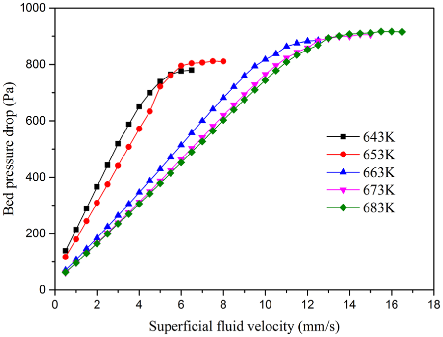
Bed pressure drop versus superficial fluid velocity.

Table 3.

Effective weight and frictional pressure drop under different conditions.

	643 K	653 K	663 K	673 K	683 K
Effective weight (Pa)	808.86	843.74	935.38	954.31	962.57
Frictional pressure drop (Pa)	779.79	811.2	885.31	904.88	915.22

The minimum fluidization velocities correspond to the turn points in the pressure drop curves in Figure 3. To make a comparison with the published empirical correlation which depended on a uniform sized particle, the particle size in this part was set as the averaged diameter. The operating pressure was set as 25 MPa. With the increment of temperature, the total pressure drop and the minimum fluidization velocity get larger, and the ratio of bed pressure drop to superficial velocity increment get lower. In particular, the changes are more drastic from 653 to 663 K, which is resulted from the great change of water properties near the critical point as shown in Table 2. Compared to the experiment data of Lu et al.,⁹ the simulated results in Figure 3 are in good agreement. In Figure 4, a comparison of the minimum fluidization velocities between the simulated results and the calculated results with Lu’s empirical correlation is made. The simulated results fit well with the empirical correlation. All the above conforms the accuracy of the CPFD method.

Figure 4.

Comparison of minimum fluidization velocities between simulated results and Lu’s work.

From Lu’s empirical correlation, it is obvious that the minimum fluidization velocity increases with the particle size. In practice, the bed materials have particle size distribution, so the transformation from fixed bed regime to fluidized bed regime is a gradual process.

Fluidization transformation with superficial fluid velocity

To study the fluidization transformation with superficial fluid velocity, the relation curve between bed pressure drop and superficial fluid velocity is an important research object. In Figure 5, it was presented that the bed pressure drop with a large ranch of superficial velocity under 25 MPa and 673 K. As this work was account for the particle size distribution in three dimensions, the simulated results of fluidization are more complicated and resemble the actual phenomenon. From Figure 5, it can be seen that the bed pressure drop curve can be divided into five stages. Besides, in Figures 6 and 7, the particle volume and size distributions in the five stages were given for further understanding:

Stage I (t = 0–30 s and U = 0–7 mm/s) corresponds to the fixed bed regime in which there is no particle reaching fluidization. In this stage, the bed pressure drop increases linearly with the superficial fluid velocity and without fluctuation.

Stage II (t = 30–52 s and U = 7–12.5 mm/s) corresponds to the gradual fluidized process mentioned in the last sub-chapter. In this stage, the pressure drop curve also increases with the superficial fluid velocity, but the rate of curve decreases with that. As can be seen from Figures 6 and 7, when the superficial fluid velocity reaches 7 mm/s, the small particles become fluidized and rise to the upper bed. On the contrary, the big particles settle down to the bottom. With the increment of the superficial fluid velocity, all the particles become fluidized gradually and the bed has a little expansion. When the superficial fluid velocity in 12.5 mm/s, the bed pressure drop is close to the total value, and it needs a much larger superficial fluid velocity to reach that. In Figure 8, the maximum particles volume fraction is less than the initial value, and the particles have been almost finished layering by the size, leaving only some big particles at the bottom. So, regarding it as the minimum fluidization velocity (u_mf) has a practical significance.

Stage III (t = 52–106 s and U = 12.5–26 mm/s) corresponds to a fluidization regime that the bed at different height expands at different rates. In this stage, particles at different heights are in different sizes and have different dynamic characteristics influenced by the superficial fluid velocity. So, mixing of particles with different size occurs and the bed fluctuates. From Figure 5, it can be seen that the pressure drop curve has a little fluctuation in stage II and III comparing to stage IV. This phenomenon in both stages is as result of particle motion. In Figures 6 and 7, there are some zones with less particle volume fraction than the surrounding ones. What’s more, the boundaries of particles with different sizes are crooked, comparing to those in stage II parallel to the bottom of reactor. In stage II, the particle volume fraction is high, so the voidage for particles’ motion is very little. Besides, the superficial fluid velocity are also very small. As a result, the expansion process is placid compared to that in stage III.

Stage IV (t = 106–154 s and U = 26–39 mm/s) corresponds to homogeneous expanded fluidization regime. The expansion process in this stage resembles to that in the previous stage. But as the fluid velocity has been much larger than u_mf, and the bed has expanded quite well, the particle volume fraction in the bed is close to uniform, which can be seen in Figure 6. It can be also gotten from Figure 5 that the pressure drop curve is much more stable in stage IV.

Stage V (t = 154–240 s and U = 39–60 mm/s) corresponds to bubbling fluidization regime. In this stage, the flow behavior is dominant by the bubble formation, coalescence, and eruption, and in Figure 6, some little bubble can be found. Besides, from Figure 7, particles with different size return to the complete mixing state. The bed pressure drop fluctuates more violently with the increase in the superficial fluid velocity.

Figure 5.

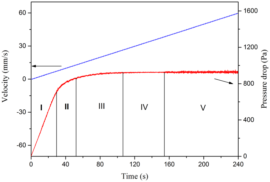
Bed pressure drop and superficial fluid velocity versus time.

Figure 6.

Particles volume fraction distribution in five stages.

Figure 7.

Particles radius distribution in five stages.

Figure 8.

Particles volume fraction and radius distribution at 12.5 mm/s.

In general, the fluidization behavior mentioned above can be concluded into three types: fixed bed regime, expanded fluidization regime, and bubbling fluidization regime. Obviously, particles in this work are categorized as Geldart B group. But from the simulated results, the minimum bubbling fluidization velocity (u_mb) is larger than the minimum fluidization velocity (u_mf), and there is a no-bubbling fluidization stage when the superficial velocity is between u_mb and u_mf. This phenomenon has been reported in many published literature.^6,19,27

Bed expansion characteristics

The bed expansion characteristic is also an important parameter for the study of fluidized bed. As shown in Figure 9, the overall voidage of SCWFB was plotted over superficial fluid velocity in a double logarithmic coordinate. From the figure, it can be seen that the bed expansion process can be also divided into five stages, which is in good agreement with the bed pressure drop curve. The minimum fluidization velocity and minimum bubbling velocity can be also determined at the turn points of the bed expansion curve. In stage I, the fixed bed regime, there is no expansion. In stage II, affected by the particle size distribution, the bed expands slightly and the expansion rate increases with the fluid velocity. When the fluid velocity is larger than the minimum velocity defined before, in stage III and IV, the overall bed voidage increases linearly with the fluid velocity in double logarithmic coordinate and the slope in the both stages has a little difference. When the fluid velocity is larger than the minimum bubbling velocity, the liner increase in the overall bed voidage versus fluid velocity disappears.

Figure 9.

The overall bed voidage versus superficial fluid velocity.

In general, Richardson and Zaki²⁸ relation is usually used to describe the bed expansion in homogeneous fluidization regime

\frac{u}{u_{t}} = ε^{n}

(12)

where u_t is the particle terminal velocity. But when the particle size distribution was taken into account, it can be seen that the bed expands heterogeneously and there exists a little turn in the expansion process. So, it needs more experimental and simulated results to describe this phenomenon.

Conclusion

SCWFB is a promising reactor for the efficient and clean conversion of coal to hydrogen. This work is aimed to make a comprehensive study of the granular flow behaviors and flow regime transformation, replenish the lack of the detail investigation inside SCWFB, and provide design and optimization basis. Main conclusions are obtained as follows:

Near the critical point of water, the minimum fluidization velocity has a larger change rate than in the other conditions.

When the particle size distribution is taken into consideration, the fluid regime transformation with the superficial fluid velocity is a gradual process. During the fluidization process, there is a particle migration and layering phenomenon, which can result in the large particle gathering in the bottom and the small one gathering in the top. So, in the practical industrial operation, the diameter range distribution of particles should not be large. And, the bottom of the bed should intensify the reacting condition.

In SCWFB, though the particles are categorized as Geldart B group, there exists a bed expansion process after incipient fluidization, rather than the bed come into bubbling fluidization immediately. In the operation of SCWFB, the superficial fluid velocity should large enough, larger than the minimum fluidization velocity, to make sure the bed in the bubbling fluidization regime with good fluidization status.

The bed expansion process is also influenced by the particle size distribution. When the superficial fluid velocity is between the minimum fluidization velocity and minimum bubbling fluidization velocity, it has a deflection that the linear increase in overall bed voidage with superficial fluid velocity in double logarithmic coordinate.

Footnotes

Appendix 1

Handling Editor: Kai Bao

Declaration of conflicting interests

The author(s) declared no potential conflicts of interest with respect to the research, authorship, and/or publication of this article.

Funding

The author(s) disclosed receipt of the following financial support for the research, authorship, and/or publication of this article: This work was financially supported by the National Key R&D Program of China (contract no. 2016YFB0600100) and National Natural Science Foundation of China (contract no. 51776169).

ORCID iD

Hui Jin

References

Jin

Zhao

Guo

et al . Experimental investigation on methanation reaction based on coal gasification in supercritical water. Int J Hydrogen Energ 2017; 42: 4636–4641.

Jin

Chen

Zhao

et al . Molecular dynamic simulation of hydrogen production by catalytic gasification of key intermediates of biomass in supercritical water. J Energ Resour: ASME 2017; 140: 041801–041805.

Matsumura

Minowa

. Fundamental design of a continuous biomass gasification process using a supercritical water fluidized bed. Int J Hydrogen Energ 2004; 29: 701–707.

Jin

Guo

et al . Hydrogen production by biomass gasification in supercritical water with a fluidized bed reactor. Int J Hydrogen Energ 2008; 33: 6066–6075.

Jin

Liao

et al . Hydrogen production by coal gasification in supercritical water with a fluidized bed reactor. Int J Hydrogen Energ 2010; 35: 7151–7160.

Liu

Kwauk

. Aggregative and particulate fluidization—the two extremes of a continuous spectrum. Chem Eng Sci 1996; 51: 4045–4063.

Vogt

Schreiber

Brunner

et al . Fluid dynamics of the supercritical fluidized bed. Powder Technol 2005; 158: 102–114.

Potic

Kersten

SRA

et al . Fluidization with hot compressed water in micro-reactors. Chem Eng Sci 2005; 60: 5982–5990.

Zhao

Han

et al . Minimum fluidization velocities for supercritical water fluidized bed within the range of 633–693K and 23–27MPa. Int J Multiphas Flow 2013; 49: 78–82.

10.

Anderson

Jackson

. Fluid mechanical description of fluidized beds. Equations of motion. Ind Eng Chem Fund 1967; 6: 527–539.

11.

Prosperetti

Tryggvason

. Computational methods for multiphase flow. Cambridge, UK: Cambridge University Press, 2009.

12.

Cundall

Strack

ODL

. A discrete numerical model for granular assemblies. Géotechnique 1979; 29: 47–65.

13.

Abbasi

Islam

Ege

et al . Downer reactor flow measurements using CREC-GS-Optiprobes. Powder Technol 2012; 224 pp. 1–11.

14.

Andrews

O’Rourke

. The multiphase particle-in-cell (MP-PIC) method for dense particulate flows. Int J Multiphas Flow 1996; 22: 379–402.

15.

Snider

O’Rourke

Andrews

. Sediment flow in inclined vessels calculated using a multiphase particle-in-cell model for dense particle flows. Int J Multiphas Flow 1998; 24: 1359–1382.

16.

Vivacqua

Vashisth

Prams

et al . Experimental and CPFD study of axial and radial liquid mixing in water-fluidized beds of two solids exhibiting layer inversion. Chem Eng Sci 2013; 95: 119–127.

17.

Liang

Zhang

et al . A critical validation study on CPFD model in simulating gas–solid bubbling fluidized beds. Powder Technol 2014; 263: 121–134.

18.

Wei

. A numerical study of bed expansion in supercritical water fluidized bed with a non-spherical particle drag model. Chem Eng Res Des 2015; 104: 164–173.

19.

Huang

Zheng

. Fluid hydrodynamic characteristics in supercritical water fluidized bed: a DEM simulation study. Chem Eng Sci 2014; 117: 283–292.

20.

Snider

Guenther

Dalton

et al . CPFD Eulerian-Lagrangian numerical scheme applied to the NETL bench-top chemical looping experiment. In: Proceedings of the 1st international conference on chemical looping, Lyon, 17–19 March 2010.

21.

Gidaspow

. Multiphase flow and fluidization: continuum and kinetic theory descriptions. San Diego, CA: Academic Press, 1994.

22.

Chhabra

Agarwal

Sinha

. Drag on non-spherical particles: an evaluation of available methods. Powder Technol 1999; 101: 288–295.

23.

Harris

Crighton

. Solitons, solitary waves, and voidage disturbances in gas-fluidized beds. J Fluid Mech 1994; 266: 243–276.

24.

Auzerais

Jackson

Russel

. The resolution of shocks and the effects of compressible sediments in transient settling. J Fluid Mech 1988; 195: 437–462.

25.

Ferziger

Peric

. Computational methods for fluid dynamics. New York: Springer, 2012.

26.

Hashizume

Morita

Kimura

. Heat transfer characteristics of liquid–solid circulating fluidized beds. Heat Transfer Eng 2011; 32: 974–980.

27.

Rhodes

Wang

Nguyen

et al . Use of discrete element method simulation in studying fluidization characteristics: influence of interparticle force. Chem Eng Sci 2001; 56: 69–76.

28.

Richardson

Zaki

. Fluidization and sedimentation—part I. Trans Inst Chem Eng 1954; 32: 38–58.

Three-dimensional numerical study on flow dynamics characteristics in supercritical water fluidized bed with consideration of real particle size distribution by computational particle fluid dynamics method

Abstract

Keywords

Introduction

Numerical method

Physical model

Simulated results and discussion

Minimum fluidization velocity

Fluidization transformation with superficial fluid velocity

Bed expansion characteristics

Conclusion

Footnotes

Appendix 1

Declaration of conflicting interests

Funding

ORCID iD

References