Sage Journals: Discover world-class research

Abstract

A growing algorithm of neural network based on axon growth is developed in this article. At the beginning, the Newtonian gravitation and the Brownian motion are employed to establish an axon growth model, and the constraint function of the neural axon growth is derived according to the gravitational coefficient and the Brown coefficient. And then, the growing algorithm of neural network is obtained on the basis of the output function of neural network. Simulation experiments show that the developed algorithm can simulate the process that different neurons connect each other by their axon growth to establish neural network. And at the end, the developed algorithm is applied to the rhythmic motion control of a quadruped robot to verify the effectiveness in walk gait and in trot gait, respectively.

Keywords

Self-growing neural network Brownian motion gravity constraint quadruped robot

Introduction

The self-growing network which follows a predetermined or dynamically adjusted policy is a goal-driven approach unlike the conventional self-organizing networks.^1,2 Axon growth is the foundation to establish the connections between neurons while developing the neuron networks.³ It can perceive the chemical information in the extra-cellular, depending on the motion of its front-end growth cone. And on this basis, axon grows to the target neuron accurately.⁴ Hence, simulating the process of axon growth can serve as the foundation for modeling the self-growing neural network. McLean et al.⁵ developed a mathematical model focusing on microtubulin. By investigating the synthesis process in neuron’s soma, the transmission along axons, and the assembling near growth cones, the relationship between neuron growth and tubulin motion is discussed. Although this model considers the mechanism of axon growth in neuron, the axon steering mechanism and the effecting factors for axon extension are ignored.⁵ Johannes and Arjen⁶ proposed a model to simulate the diffusion process of chemical molecules in the growth environment by partial differential equations (PDEs) and ordinary differential equations (ODEs). The extension and the steering of axon in this model are considered as the distribution function of molecular concentration.⁶ However, it lacks the corresponding biological validation and also causes the large amount of calculation. Randal et al.⁷ proposed a simplified single-neuron growth model by describing the extension, the steering, and the bifurcation of axon as stochastic motions. Even the simplified model can approximate the synaptic distribution and the behavior of axon bifurcation in biological neural network from the aspect of morphology; the network generated by this model lacks the functions of biological neural network,⁷ and so far, there is little public report on effective motion control of quadruped robot using the above models.

The above-mentioned models have a common problem that the axon growth and the connecting structure of network cannot be constrained to obtain neural network with specific functions. It is also the main challenge in self-growing neural network. Zubler and Douglas⁸ developed a diffusion model of chemical molecules in the growth environment by the geometrical method and then proposed a mechanical model by describing the axon growth to approximate the neural network in cerebral cortex from the view of morphology. Even though it has shortcomings such as that the generated neural network lacks some characteristics of biological neural network, this approach still inspires us to introduce mechanics into the research of self-growing network. In this article, the universal gravitation is employed to describe the targeted effect from soma to growth cone, and the stochastic motion is employed to describe the noise while the growth cone is steering in the growth environment.^9,10 Then, the axon growth model (a set of equations describing the general growth process of axon) based on the Newtonian gravity and the Brownian motion (the erratic random movement of microscopic particles in a fluid, as a result of continuous bombardment from molecules of the surrounding medium) is developed. By analyzing the gravitation coefficient and the Brownian coefficient, the constraint function of axon growth can be obtained. The neural network with motion control capability can be generated by connecting multiple neurons via different axon growth.

The remainder of this article is organized as follows. Section “Self-growing model of neuron axon” develops a goal-driven model of growth cone based on the gravitation and the Brown motion. Here, the gravitation is introduced to describe the goal-driven effect of target neuron soma on growth cone. In section “A growing algorithm of neural network,” it is detailed that when the motion of growth cone is controlled, the share of deterministic motion caused by gravitation and the stochastic motion caused by Brownian motion can be served as the constraint on the movement of growth cone. And it should be noted that the self-growing algorithm of neuron network is developed to realize the controllable growth. The developed algorithm covers the connection and the output of neuron network. Section “Results and discussion” details the experiments that rhythmic movements of quadruped robot are controlled by the developed self-growing algorithm when robot walks and trots and this is the first time self-growing network is applied to legged robot. Finally, section “Conclusion” contains the conclusion drawn from this study.

Self-growing model of neuron axon

According to the neurobiological studies,¹⁰ axon growth process can be simplified into three crucial steps by external chemical guiding molecules as shown in Figure 1.

The direction of tubulin perception. The concentration distribution of external chemical molecules is converted into the corresponding internal ligand concentration distribution by tubulin in growth cone as shown by the pink line in the left subgraph of Figure 1.

The movement of filopodia. It is along the direction of gradient driven by the flow of actin in growth cone as shown by the middle subgraph of Figure 1.

The Polarization of axon. New axon segments are generated by the polarization of the back of growth cone along the movement direction of the front of growth cone as shown by the right subgraph of Figure 1.

Figure 1.

The schematic diagram of axon growth process. The orange solid circles represent target neurons.

According to the above three steps, an axon growth model including three modules, that is, perception module, motion module, and growth module, is developed.

Perception module

The guidance effect of chemical molecules in external environment on the growth cone can be described as a force action.^11,12 Hence, the main function of perception module is to simulate the spatial distribution of chemical guiding molecules, that is, to calculate the guiding force on the growth cone using the concentration field. For the complexity of concentration field, the gravitational field is introduced to simulate the concentration field and calculate guiding force. This approach provides two advantages that it can reduce computational complexity effectively and gain the guiding force on the growth cone via Newtonian gravity formula directly.

The steady-state diffusion of molecules and the potential distribution in the gravitational field are given by equations (1) and (2), respectively

D Δ u = W (x, y, z)

(1)

where u represents the concentration field, △ represents the Laplace operator, D represents the diffusion coefficient, and W(x, y, z) represents diffusion sources

{\begin{matrix} \frac{1}{4 π k} Δ U = ρ (x, y, z) \\ U = - s \frac{M}{r^{2}} \end{matrix}

(2)

where ρ(x, y, z) represents the density of the material source, k represents the constant coefficient, U represents the gravitational potential, s represents the gravitational coefficient, r represents the length vector, and M represents the total mass of the field source material.

Comparing equation (1) with equation (2), it finds that the steady-state diffusion of molecules and the potential distribution in the gravitational field satisfy the Poisson equation. Hence, for concentration field distribution generated by different D and W in equation (1), it always finds a set of s and M to make the distribution of U in equation (2) equals to the distribution of u in equation (1). For example, when W = 15 mmol/L, D = 0.5 in equation (1), and s = 0.05 m³/(kg s²), M = 20 mg in equation (2), and the distributions of u and U are shown in Figure 2.

Figure 2.

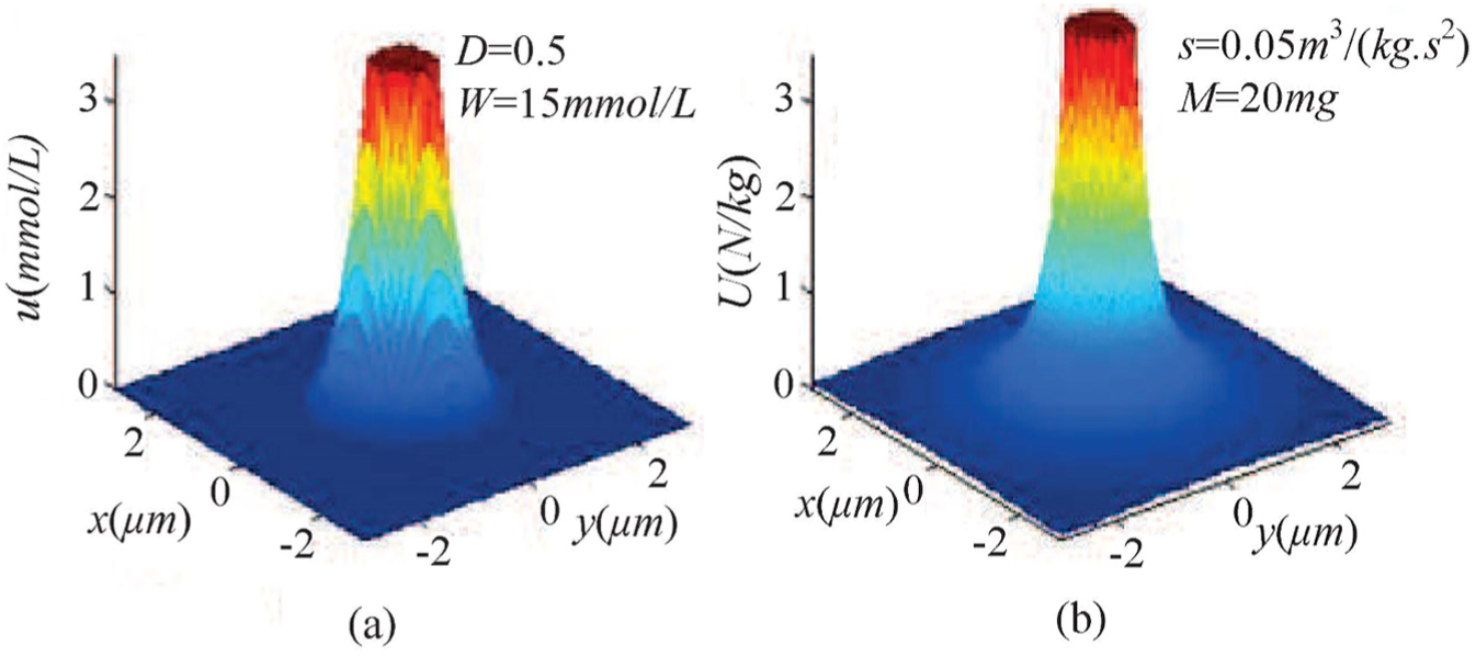
Distribution diagrams for concentration field and gravitational field: (a) distribution of the concentration field u and (b) distribution of the gravitational potential U.

As shown in Figure 2, the concentration distribution u and the gravitational potential U have similar amplitude and distribution radius. From another point of view, both the gravitational field and the concentration field meet the linear superposition principle. Hence, the vector synthesis method is acceptable for multiple gravitational fields and multiple concentration fields.^13–15 It is reasonable to simulate the concentration field of chemical molecules using the gravitational field.

If there are k-field sources in gravitational field, the suffered gravity of the growth cone whose mass is m could be written as equation (3) according to Newton’s law of gravitation

P = \sum_{j = 1}^{k} \vec{F_{j}} = \sum_{j = 1}^{k} s_{j} m \frac{M_{j}}{d_{j}^{2}} \vec{e_{j}}

(3)

where d_j represents the distance between the growth cone and jth neuron, $\vec{e_{j}}$ represents the direction vector of the gravity between the jth neuron and the growth cone, m represents the mass of the growth cone, and M_j represents the jth neuronal mass. s_j represents the gravitation coefficient of jth neuron. The gravity value P, which represents the perception module output, describes the goal-driven effect of target neuron soma on growth cone: target neuron, through its own gravitation, influences the growing direction and velocity of growth cone and guide axon growth to the source of gravitational field.

Motion module

The motion state of the growth cone is calculated by motion module based on the gravity value P obtained by perception module. The corresponding motion equation is given by equation (4)

m {\overset{\cdot\cdot}{X}}_{s} = P

(4)

where X_s = X_s(x, y) represents the growth cone coordinate in the two-dimensional gravitational field. Denote time interval as Δt and start time as k. After Δt, the motion of the growth cone at time k+1 can be given by equation (5)

{\begin{matrix} α^{k + 1} = \frac{P}{m} \\ V^{k + 1} = α^{k + 1} Δ t + V^{k} \\ Δ X_{s}^{k + 1} = \frac{1}{2} α^{k + 1} Δ t^{2} + V^{k} Δ t \\ Δ s^{k + 1} = \sqrt{{(Δ x^{k + 1})}^{2} + {(Δ y^{k + 1})}^{2}} \\ θ_{D}^{k + 1} = \tan^{- 1} (\frac{Δ y^{k + 1}}{Δ x^{k + 1}}) \end{matrix}

(5)

where α^k+1 and V^k+1 represent the motion acceleration and the velocity vector, respectively; $Δ X_{s}^{k + 1} = (Δ x^{k + 1}, Δ y^{k + 1})$ represents the single-step growing displacement, Δs^k+1 represents the position vector norm of the growth cone at time k+1, and $θ_{D}^{k + 1}$ represents the angle between the positive direction of x-axis and the growth cone at time k+1.

The growth step Δs^k+1 and the angle $θ_{D}^{k + 1}$ of the growth cone from the time k to time k+1 can be provided by the motion module. For the calculation at time k+2, the growing rate V^k+1 of the growth cone needs to be outputted to the motion module at the next step.

Growth module

The axon growth within a time interval is completed by growth module based on motion module. Considering Pearson’s research results and the randomness of biological neuron growth process,⁹ it is possible to study the randomness of axon growth by Brownian motion.

The randomness of axon growth mainly displays in its motion directions. In the condition of infinitesimal step, the random deflection angle can be described by equation (6)

d θ_{s} (s) = c \cdot d B_{θ} (s)

(6)

where θ_s represents the random deflection angle, B_θ(s) represents Brownian motion, c represents Brownian coefficient, and s represents the arc length of the axon. Computing the integral of equation (6) yields equation (7)

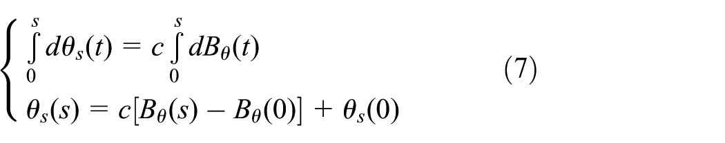
{\begin{matrix} \int_{0}^{s} d θ_{s} (t) = c \int_{0}^{s} d B_{θ} (t) \\ θ_{s} (s) = c [B_{θ} (s) - B_{θ} (0)] + θ_{s} (0) \end{matrix}

(7)

while s = 0, the initial values of θ_s(0) and B_θ(0) are set to 0. As shown in equation (8), the increment of Brownian motion is independent and normally distributed. The mean value is 0 and the variance is constant

[B_{θ} (s) - B_{θ} (0)] ~ N (0, s)

(8)

where N represents the normal distribution, the mean value is zero, and the variance is s.

The obtained random deflection angle θ_s is as follows by solving equation (9)

θ_{s} (s) ~ N (0, c^{2} s)

(9)

The random deflection angle $θ_{s}^{k + 1}$ from time k to time k+1 can be written as equation (10) by discretization

θ_{s}^{k + 1} ~ N (0, c^{2} Δ s^{k + 1})

(10)

The total deflection angle θ^k+1 of the growth cone at time k+1 can be described by considering the certain deflection angle $θ_{D}^{k + 1}$ in equation (5) and the random deflection angle $θ_{s}^{k + 1}$ in equation (10), as shown in equation (11)

θ^{k + 1} = θ_{D}^{k + 1} + θ_{s}^{k + 1}

(11)

Hence, the new position vector $X_{s}^{k + 1} (x^{k + 1}, y^{k + 1})$ of the growth cone can be given by equation (12)

{\begin{matrix} x^{k + 1} = x^{k} + Δ s^{k + 1} \times \cos (θ^{k + 1}) \\ y^{k + 1} = y^{k} + Δ s^{k + 1} \times \sin (θ^{k + 1}) \end{matrix}

(12)

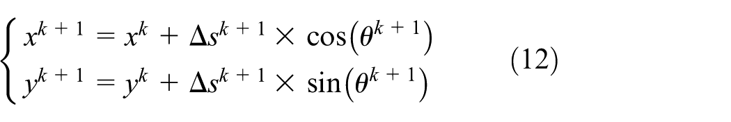
Axon growth segments from time k to time k+1 can be obtained by connecting $X_{s}^{k}$ to $X_{s}^{k + 1}$ . This process is seen as a single-step growth of axon. To compute the iterative process at time k+2, the position vector $X_{s}^{k + 1}$ at time k+1 needs to be outputted by the growth module.

As mentioned above, the continuous growth of axon is performed by the iteration loop of three modules as shown in Figure 3.

Figure 3.

Flowchart of the axon growth model. r_c represents the radius of the cell body.

In Figure 3, r_c represents the radius of the cell body which is simplified as a circle for calculation convenience. First, according to the gravitational potential U and the distance d between the growth cone and target neuron, the sensing module outputs the gravity value P into movement module to get input parameters Δs^k+1 and $θ_{D}^{k + 1}$ for growing module. Second, based on the position vector $X_{s}^{k + 1}$ at time k+1 given by growing module, the axon connection can be completed when the distance d between the growth cone and the target neuron is less than or equal to the radius r_c of the cell body. Otherwise, start iterative process at time k+2 from sensing module to growing module.

A growing algorithm of neural network

Growth constraint of the neuron axon

The accurate and efficient connections among neurons are the foundation of neural network growth. It determines the function of neural network. Hence, it is crucial to constrain the axon growth.

In order to simplify the calculation, neurons are arranged symmetrically as shown in Figure 4. In this case, the neurons located on symmetrical positions share the same growth environment and follow the same growth rule, so the computational complexity goes down. Assume that the growth region of neural network is a square whose side length is 20 unit lengths and the circle with different numbers serves as neuron. After the selection of the origin point in the two-dimensional coordinate system, the coordinates determine the neuron position uniquely. A particle randomly generated by neuron in the direction from 0° to 360° serves as the growth cone. Each neuron generates a growth cone which is represented by particle in the direction from 0° to 360° randomly. The motion trajectory of the growth cone in two-dimensional gravitational field is the axon of that neuron. Each neuron generates only one axon to connect with another neuron as shown by the dashed lines in Figure 4. The neurons in Figure 4 are divided into the following four classes.

Class 1: No. 1, No. 2, No. 3, and No. 4 neurons in the four corners are of output control function.

Class 2: No. 5, No. 8, No. 10, and No. 13 neurons are on the vertex positions.

Class 3: No. 6, No. 7, No. 11, and No. 12 neurons are on the midpoint of the edge.

Class 4: No. 9 neuron is in the center of the neurons.

Neurons from No. 5 to No. 13 are intermediate neurons. The pathway of signal transmission is determined by connecting output neurons and intermediate neurons. According to equations (6) and (13), the trajectory of axon generated by each neuron and the target neuron of its axon is related to the gravitational coefficient s determined by other neurons and the Brown coefficient c determined by the axon itself. Hence, a certain neuron can be connected with the specific neuron by controlling the gravitational coefficient s_ij between neuron i and neuron j. It provides the opportunity to establish a network with specific function and control the connections among neurons to some extent.

Figure 4.

Distribution of neurons.

Take as an example of No.5 and No.1 neurons. Count up the total number of connections for each s₅₁ as shown in Figure 5. Even if the movements of growth cones are uncertain for introducing the Brownian motion. It also means that the ultimate connected target of each neuron axon is uncertain. In this case, a stable connection between specific neurons can be ensured by increasing the value of s. For example, in Figure 4, when the gravitational coefficient between No. 1 neuron and No. 5 neuron is 20, the connection probability between the two neurons is almost close to 0 even though the simulation was repeated many times. When 20 < s₅₁ < 70, the connection probability increases approximately linearly as shown in Figure 5. The axon of No. 1 neuron can connect to No. 5 neuron almost every time when s₅₁ > 80. Hence, as can be seen from Figure 5, the connection probability between No. 1 neuron and No. 5 neuron grows with the increase in s₅₁, and it is almost equal to 1 to achieve a reliable connection when s₅₁ > 80.

Figure 5.

The relationship between the connection probability and the gravitational coefficient. The blue solid line illustrates the connection probability when 10 ≤ s₅₁. The blue hollow circle illustrates the connection probability when s₅₁ = 10, 20, …, 100.

Similarly, the change of connection probability of other neurons related to the gravitational coefficient is analyzed via Figure 4, and then, s values for reliable connections of other different neurons are obtained in Table 1.

Table 1.

Lower limited values of the gravitational coefficients when different types of neurons connect reliably.

Classes of neuron	Class 1	Class 2	Class 3	Class 4
Class 1	−	80	60	−
Class 2	80	−	50	70
Class 3	60	50	80	50
Class 4	−	70	50	−

According to equation (3) and Figure 5, the magnitude of gravitation is related to the distance between growth cone and target neuron, and a reliable connection between them is related to the gravitational coefficient. As shown in Figure 5, the connection between neuron class 1 and class 2 is reliable when s ≥ 80. Similar experiment shows that s values for reliable connections between neuron class 1 and class 3, class 3 and class 3, class 2 and class 4, class 2 and class 3, and class 3 and class 4 are s ≥ 60, s ≥ 80, s ≥ 70, s ≥ 50, and s ≥ 50.

Take the case of the connection between No. 1 neuron and No. 5 neuron to study the relationships among the axon growth length, the probability, and the Brown coefficient. Denote the axon length as L in the case of maximum probability. L is the expected axon length according to normal distribution. Then, Figure 6 shows the change in Brownian coefficient c, and the growing probability of different axon is obtained by statistic. The unit of length is 10 μm in Figure 6.

Figure 6.

Relationships among the axon growth length, the connection probability, and the Brownian coefficient. (a) The relationship between the expected axon length L and the Brownian coefficient. When c₅₁ is given, the axon length is between 9 and 15 and the occurring probability of corresponding length goes down as the length value increases. (b) The probability of expected length L for different axon. The expected axon length increases gradually as the Brownian coefficient grows. The range of blue circles represents the data range of axon length, and the red solid line is the fitting curve of expected axon length values.

According to Figure 5 and Table 1, the gravitational coefficient s₅₁ is set to 80 to ensure the axon of No. 1 neuron grows to No. 5 neuron successfully every time. The Brownian coefficient c₅₁ varies from 1 to 5 and the increment is 0.2. Then, the simulations were done for 5000 times. The relationship between the axon growth length and the Brownian coefficient is illustrated in Figure 6(b) according to the statistics of simulation results. The axon growth length and its variation range increase with c₅₁ going up. This is because the growing of c₅₁ leads to the increase in variation range of random steering angel $θ_{s}^{k + 1}$ according to equations (11)–(13) and then evokes a bigger turning on the growth axon. The turning can increase the axon length and its variation range. Calculate the probability of expected axon length in Figure 6(b) by p(L) = n(L)/n where p(L) is the probability of expected axon length L, n(L) is the frequency when axon length approximates to L, and n is the number of simulations (n = 5000 in this article). The obtained probability of expected axon length L is shown in Figure 6(a). It is easy to find that the probability goes up as expected and axon length L decreases and reduces gradually with the increase in L.

Fitting the simulation results shown in Figure 6, equations (13) and (14) are obtained

L (c) = a_{1} \cdot c^{b_{1}} + d_{1}

(13)

P (L) = a_{2} \cdot L^{b_{2}} + d_{2}

(14)

where a₁ = 0.1303, b₁ = 2.526, d₁ = 8.993, a₂ = 13,730, b₂ = –5.29, and d₂ = 0.03115. The constraint of Brownian coefficient c relative to the expected axon length L is established by equation (14). The fitting results are shown by the red solid lines in Figure 6(a) and (b). Similarly, the relationships between expected axon lengths of other neurons in Figure 4 and the Brownian coefficient c are illustrated in Table 2.

Table 2.

The value range of expected axon length L between different types of neurons and the coefficient value of constraint function.

Category of growth neuron	Constraint function coefficient			Value range of axon length L_mp	Category of target neuron
Category of growth neuron	a ₁	b ₁	d ₁	Value range of axon length L_mp	Category of target neuron
Class 1	0.1303	2.526	8.993	9.0–16.3	Class 2
Class 1	0.0767	2.635	6.892	6.8–14.9	Class 3
Class 2	0.1361	2.515	9.066	9.1–17.4	Class 1
Class 2	0.05366	2.763	5.529	5.5–11.1	Class 3
Class 2	0.1299	2.408	7.675	7.7–14.1	Class 4
Class 3	0.08478	2.572	6.81	6.8–14.2	Class 1
Class 3	0.08175	2.49	5.379	5.4–11.0	Class 2
Class 3	0.1665	2.239	7.627	7.8–11.9	Class 3
Class 3	0.07301	2.524	5.361	5.3–11.6	Class 4
Class 4	0.123	2.432	7.73	7.7–13.6	Class 2
Class 4	0.06442	2.594	5.37	5.3–11.0	Class 3

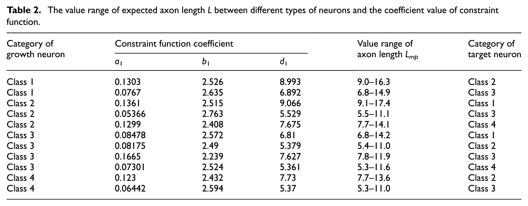
As mentioned earlier, the constraints of the gravitational coefficient s and the Brownian coefficient c relative to growths of different neuron axons shown by Tables 1 and 2 and equation (14) are obtained via simulations in Figures 5 and 6. It lays the foundation for studying relative accurate targeting growth of neuron axon.

Connection algorithm of the neural network

The key for getting reasonable and effective bioelectricity signals from neural network is finding out the reliable connections among output neurons. When the connection lengths are determined, the intermediate neurons are needed to build the corresponding connections.

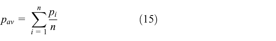
The formation process of neuron connections from the start of neuron axon growth to the reliable connection with target neuron is analogous to the target search process first. The breadth-first search (BFS) algorithm is adopted to search all the possible connections.^16,17 To evaluate the realizability of possible connection, the average probability p_av is defined as evaluation parameter by equation (15)

p_{av} = \sum_{i = 1}^{n} \frac{p_{i}}{n}

(15)

where p_i represents occurrence rate of the ith axonal growth and n represents the neuron number in complete network. As the accurate connection among neurons is a probability event, the more neurons are located on the connections and the less available connections are formed. To maximize the average probability of each connection, the distribution of axon lengths on connection is necessary to be optimized.

Assuming that the neuron number on the connection is m, the sum of expected axon lengths L, the allowable error ΔL, the value range of each axon length l_i, and the corresponding distribution function of occurrence rate P_i(x) are known. And then, the average probability on this connection can get the maximum value in the case of satisfying the expected length by optimizing the axon length x = (x₁, x₂, …, x_m_– 1) as shown in Figure 7.

Figure 7.

Schematic diagram of connecting optimization. For each available signal transmission path found by BFS algorithm, neurons from No. 1 to No. m located on the path may belong to the different four classes of neurons mentioned earlier.

Selecting an appropriate gravitational coefficient according to Table 1 makes two adjacent neurons form a reliable connection whose formation probability is close to 1. The total expected length L on this connection is divided to each segment axon from x₁ to x_m_– 1. The distribution rule is to maximize the average probability determined by equation (15) to gain the fastest growth speed. Figure 7 illustrates that each axon segment length x_i corresponds to a probability P_i(x) and the length x_i relates to the Brownian coefficient c_i. Hence, the values of c₁ to c_m_– 1 are determined through the relationship between x_i and c_i after the optimized axon length distribution x_i is obtained by equation (16). Then, the constraint for the connection of neural network is achieved by the gravitational coefficient s and Brownian coefficient c

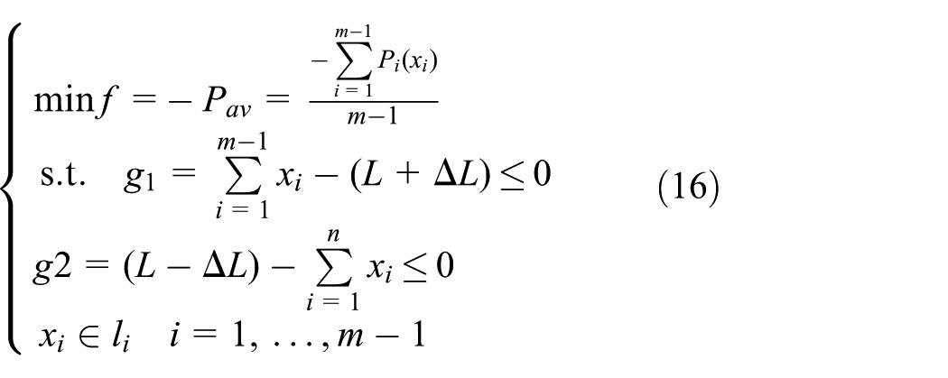
{\begin{matrix} min f = - P_{av} = \frac{- \sum_{i = 1}^{m - 1} P_{i} (x_{i})}{m - 1} \\ \begin{matrix} s . t . & g_{1} = \sum_{i = 1}^{m - 1} x_{i} - (L + Δ L) \leq 0 \end{matrix} \\ g 2 = (L - Δ L) - \sum_{i = 1}^{n} x_{i} \leq 0 \\ \begin{matrix} x_{i} \in l_{i} & i = 1, \dots, m - 1 \end{matrix} \end{matrix}

(16)

where f represents the optimized objective function and g₁ and g₂ represent inequality constraint functions. g₁ and g₂ are solved by the discrete variable optimization algorithm based on the relative difference quotient method. The relative difference quotient method starts from the minimum of the objective function f outside the feasible set, finds the rule that has the minimum increment of objective function and the maximum reduction of constraint function to satisfy all the constraint functions and gain the minimum value of objective function.¹⁶

Output function of the neural network

A complete connection can be obtained among the output neurons by the constraint function mentioned above. Then, the output function of neural network for exporting the specific control signals is studied based on this complete connection.

The relationship of phase sequences among output signals is one of the macroscopic characteristics for neural networks. Hence, the relative relationship of connection lengths among output neurons is converted to the relative relationship of phases of output signals to build the output function. Assume that the average rate of signal transmission is a constant. In this case, the phase difference φ between output signals of output neurons is proportional to the difference of total axon lengths on the connections. The distributions of connection lengths are calculated for all the possible connections from No. 1 output neuron to No. 2 output neuron, from No. 1 output neuron to No. 3 output neuron and from No. 1 output neuron to No. 4 output neuron as shown in Figure 4. The connection lengths are discretized, and the corresponding connection number is recorded. Denote the connection number as the frequency number. Then, the probability distribution function F(x) is obtained by the histogram of x as shown in Figure 8.

Figure 8.

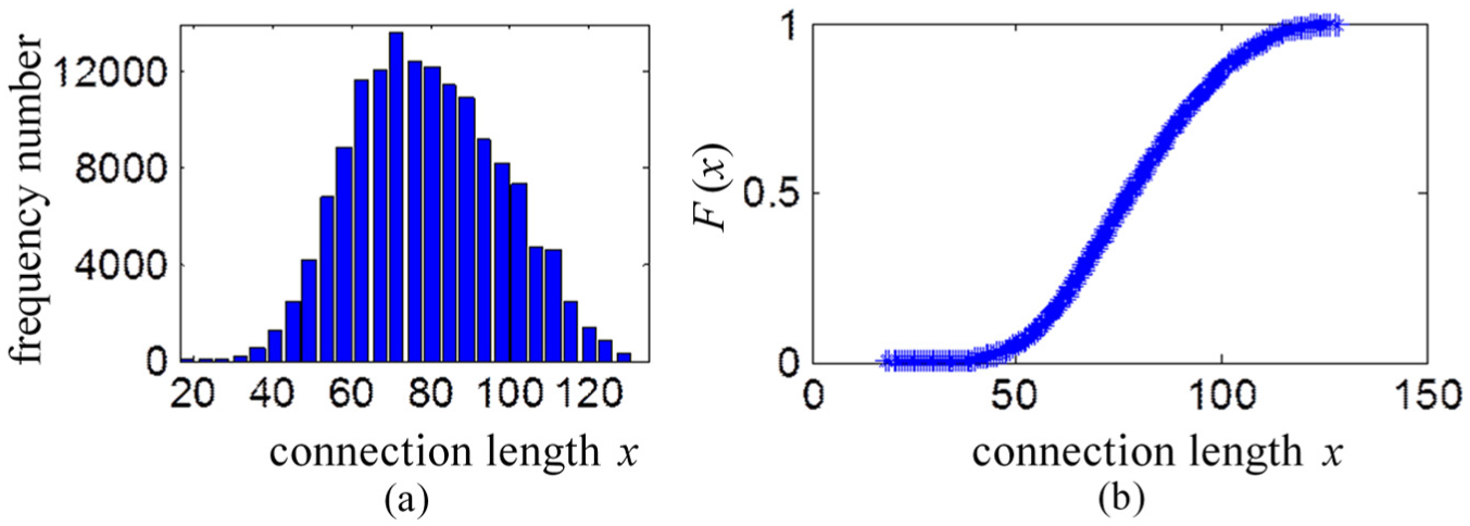
The length distribution of possible connections: (a) the frequency distribution of connection lengths and (b) the distribution function F(x).

For the network growth environment of Figure 4, all the possible connections among outputs neurons are searched by the breadth-first algorithm. For each connection, the gravitational coefficient is chosen as in Figure 7, and the Brownian coefficient increases from 1 to 5 with the increment of 0.2. The distribution of all the possible connection length x among output neurons can be obtained through a large number of axon growth simulations. As shown in Figure 8, x basically meets the normal distribution, and the probability distribution approximates to S-shaped curve.

Figure 8(a) illustrates that the probability distribution for connection length x which is from 18.1 to 129.3 approximates to normal distribution. In addition, the probability distribution for the median gets the maximum value which indicates that the corresponding connection number is maximal, and the probability distributions for the two ends get the minimum value which means the corresponding connection number is relatively small. If the linear transformation of phase difference between the connection length and the oscillating signal is done directly, the distribution of connection numbers corresponding to the phase difference is not homogeneous. To solve this problem, the connection length is transformed into the S-shaped function by the distribution function F(x) and fitted by the exponential function. Then, the output function is obtained by the linear transformation of phase difference between the connection length and the oscillating signal as shown in equation (17). x represents the axon length, φ represents the phase difference between the oscillation signals. Define the mean value of x as x_av, when x is less than or equal to x_av, λ₁ = 1 and λ₂ = 0. When x is greater than x_av, λ₁ = 0 and λ₂ = 1. The other fitting parameters are as follows: a₃ = 0.9733, a₄ = 0.2974, a₅ = 1.129, b₃ = 122, b₄ = 83.06, b₅ = 76.52, c₃ = 36.28, c₄ = 23.42, c₅ = 14.01, and d₅ =−0.09383

\begin{matrix} φ (x) = 360 λ_{1} {a_{3} \exp [\frac{- {(x - b_{3})}^{2}}{c_{3}^{2}}] \\ + a_{4} \exp [\frac{- {(x - b_{4})}^{2}}{c_{4}^{4}}]} \\ + 360 λ_{2} {\frac{a_{5}}{1 + \exp [\frac{- {(x - b_{5})}^{2}}{c_{5}}]} + d_{5}} \end{matrix}

(17)

The distribution of frequency for phase differences after mapping of output function is illustrated in Figure 9.

Figure 9.

The distribution histogram illustrates the frequency and the phase differences among output neurons after mapping of output function (equation (17)). j represents the phase differences among all the possible signals of output neurons.

By comparing Figures 8(a) and 9, the uniform distribution of the frequency and the phase difference for output neurons can be found after mapping of output function. The reason for obtaining a uniform distribution is that the connection generated from the neural network should have no preference with the phase difference between the output neurons. In other words, no matter how much the phase difference between the output neurons is, the possibility of gaining the required connection generated by the neural network is the same.

Parameter analysis

The time interval Δt and random rotation angle θ_s

The motion trajectory of growth cone is the neuron axon, so growing step length Δs and deflection angle θ of the growth cone are very important. On one hand, according to equation (5), the growing step of growth cone is proportional to time interval Δt, that is, the longer the Δt, the larger the growing step. On the other hand, the deflection angle θ of growth cone is the composition of the determined rotation angle θ_D resulted from the gravitational field and the random rotation angle θ_s generated by random motion. First, according to equation (5), the determined growing direction of growth cone is always oriented to the center of target neuron under the influence of the gravitational field. Denote the angle between the positive direction of x-axis and the connecting line between the growth cone and the target neuron as α, and then, the determined rotation angle θ_D will gradually approach α under the influence of the gravitational field. Therefore, θ_D mainly depends on the distribution of gravitational field and the position of growth cone, independent of time interval Δt. Second, according to equation (10), the variance σ of random rotation angle θ_s is proportional to growing step Δs, that is, variance σ of θ_s will increase when time interval Δt becomes larger. Therefore, in theory, the time interval Δt mainly affects the growing step and the random deflection angle of growth cone.

When the time interval Δt is 0.005, 0.02, and 0.05 s, the coordinate locations of growth neuron and target neuron are (0,0) and (3,3) respectively; the initial velocity v₀ of growth cone is (0,2), the maximum velocity amplitude v_max = 10, Brownian coefficient c = 1, and gravitational coefficient s = 10, and we finished growing experiment 100 times for each time interval Δt mentioned above, drew the statistic distribution of random deflection angles, and plotted 20 trajectories of them, as shown in Figure 10.

Figure 10.

The growing trajectories of axon growth for different time intervals Δt.

The top row in Figure 10 shows the distribution histogram of the random deflection angle θ_s for each time interval Δt. As shown in Table 3, the mean value, standard deviation, and upper and lower limits corresponding to the 95% confidence interval for θ_s were calculated. It can be seen that θ_s approximates a normal distribution. And as the time interval increases, the standard deviation and the upper and lower limits of θ_s also increase, while the mean value remains substantially near zero.

Table 3.

Variation parameters of random deflection angle θ_s.

Parameters of θ_s	Time interval Δt
Parameters of θ_s	0.005 s	0.02 s	0.05 s
Mean (°)	−0.134	−0.782	1.582
Variance (°)	9.152	18.651	31.356
Upper limits (°)	19.940	40.682	61.425
Lower limits (°)	−19.940	−42.348	−60.832

The bottom row in Figure 10 shows the 20 axonal trajectories for each time interval Δt. When Δt = 0.005 s, all the 20 axons can eventually grow to the position where the target neuron is located. These axons are distributed in a narrow area and axon shape changes gently. However, as Δt increases, the distribution area of axons rapidly increases, the abrupt change of axon shape becomes more and more obvious, and spatial resolution also decreases. This variation law is consistent with the Johannes and Arjen.¹⁸

In summary, as the time interval Δt increases, the spatial resolution of axon trajectories will decrease and abrupt change of axon trajectories will be greater. As a result, the axon trajectories will cross the target neuron cell body and cannot be connected with it. However, the decrease in time interval will result in the increase in neuron growth iterations and computation time. Therefore, in order to balance the contradiction between the higher spatial resolution and smoothness of neuron axons and short calculation time, the time interval Δt is set to 0.005 s.

The gravitational coefficient s

Currently, a common way to verify the effectiveness of the neural growth model is to compare the biological neuron growth results with the simulation results of model as the reasonable neural growth models have high similarity with biological neurons from the view of morphology.^19,20 Hence, this subsection provides the simulation focusing on single-neuron growth to evaluate the neuron growth model based on Newtonian gravity and Brownian motion, extracting the corresponding morphological features to compare with the existing research results.

The well-known experiment in neurobiology field is to observe neuron growth process while the single repulsive chemical molecule source is given. According to this approach, a neuron with repulsive function is given to simulate the induction effect. Considering the research method of Kobayashi et al.,¹⁰ the growth region is divided into the strong interaction region SR and the weak interaction region WR. In these two regions, the ratios of the axon areas to the entire region, defined as pSR and pWR, respectively, are calculated as shown in Figure 11.

Figure 11.

Distribution diagram for SR and WR.

Denote the diameter of neuron soma as a benchmark, and convert all the lengths to dimensionless values. Generally the diameter of neuron soma is 5∼150μm.^19,20 Assume that the unit length is 10 μm. In the growth area in Figure 11, the position coordinates of the growth neuron and the target neuron are (1, 5) and (5, 5), respectively. The initial velocity of the growth cone is 1 and the directions distribute randomly from 0° to 360°. The Brownian coefficient c is 3, and the gravitational coefficient s increases progressively from −3.5 to −0.5 with the increment 0.5. For each s, 1000 experiments were done. Each experiment was repeated 300 times with the same s. The simulation results are shown in Figure 12(a)–(c). It can be seen that, while s < 0, the synaptic repulsive force of the target neuron relative to the growth neuron increases as s goes down, and the growing synapse is far away from the target neuron. This illustrates that while one of the neurons fails,^21,22 the gravitational coefficient of this neuron is less than 0, and the growing synapse tends to move away from this neuron.

Figure 12.

Statistical values of pSR and pWR changing with the gravitational coefficient s under the condition of repulsion. The box represents the interquartile range of values, the line in the box represents the median. Whiskers above and below the box represent the 90th and 10th percentiles, respectively. The left blue box plots represent simulation data whose distributions vary with different values of s, and the right red box plots represent results obtained by Kobayashi et al. through the biological experiments (BERs). (a) The growth result of synapse while s = −1. (b) The growth result of synapse while s = –2. (c) The growth result of synapse while s = −3.5. (d) The relationship between pSR and the gravitational coefficient. (e) The relationship between pWR and the gravitational coefficient.

By analyzing Figure 12(a)–(c), pSR and pWR can be obtained as shown in Figure 12(d) and (e). It is clear that when the gravitational coefficient s is −3.5, the average value of pSR is close to the biological experiment results. pSR reduces gradually while the gravitational coefficient increases, and conversely, pWR gradually increases as shown in Figure 12(e).

The average values of pWR are almost equal to the biological experiment results when s = –3 or s = –2.5. It is thus clear that the simulation results obtained by developed model are consistent with biological data. This further illustrates the rationality of the developed model.

According to the algorithm flowchart shown in Figure 3 and considering equations (6) and (12), the growth simulations from axon to target neuron can be obtained as shown in Figure 13 while s = 1, 2, and 3.5. It illustrates that more axons move toward to the centre of target neuron as the attraction effect of target neuron on axon becomes greater. It also illustrates that, the axon is more likely to grow to target neuron while s increases.

Figure 13.

The neuron growth in different attraction intensity.

Figure 13(d) and (e) is derived from the simulation results of Figure 13(a)–(c). It illustrates that while s > 0, pSR grows with s increasing. Conversely, pWR goes down. These simulation results further indicate that guiding neuron axon by Newtonian gravitation is acceptable.

Experiment plot

Modern manufacturing style demands industrial-level mobile manipulation robotic technology featured with task flexibility and robotic mobility and learning ability.²³ Technologies, such as teleoperation^24–26 and neural learning²⁷ for mobile manipulation, have been widely studied and applied on robotic mobile platforms. As a major component sector of robot, the legged robot is one of the most versatile design strategies for such robotic mobile platforms.

Therefore, the quadruped robot is selected as the control object as it plays the significant role in the field of robotics. According to the physiological structure of four-legged animal, the simplified model of quadruped robot is designed as shown in Figure 14. Each leg has three rotating joints, that is, hip joint α, knee joint β, and ankle joint θ. Other parameters are illustrated in Table 4.

Figure 14.

The model of quadruped robot.

Table 4.

Parameters of quadruped robot.

Parameter	Numerical value
M (kg)	67
L₁ (m)	0.680
L₂ (m)	0.450
l₁ (m)	0.233
l₂ (m)	0.233
l₃ (m)	0.310

The computer system parameters are as follows: CPU (i5 4690K, 4-core, 3.5 GHz), Internal memory (8G, DDR3), video card (2048 MB, DDR5, and 128 bit), and hard disk (500 GB).

Results and discussion

The quadruped robot moves rhythmically and depends on the motion phase sequence of hip joint to achieve different gaits.²⁸ To gain the rhythmic movement of quadruped robot, the Van der Pol oscillator is employed to generate the periodic oscillating signal of output neuron. The neural network in Figure 13(b) is integrated in the quadruped robot. Output neurons of the network are connected with hip joints as shown in Figure 15. The No. 1, No. 2, No. 3, and No. 4 neurons control the left front (LF), the right front (RF), the right hind (RH), and the left hind (LH) of the hip joint, respectively. The control signal of output neuron corresponds to the angular displacements of hip joint.

Figure 15.

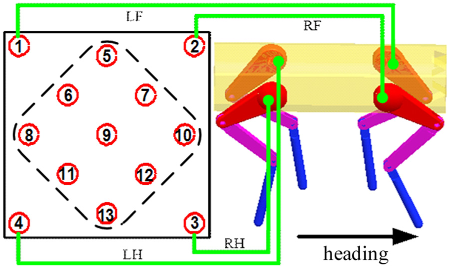
Schematic diagram of the fusion between neural network and quadruped robot.

Walk and trot are common phenomena in various giants for quadrupeds.^17,29–31 Hence, the two gaits are discussed in this section. Different gait corresponds to different hip joint, and the phase of displacement curve of each hip joint is different. To facilitate the analysis, assume that the displacement curve has the form of sine wave. Define the hip joint of LF corresponded to No. 1 neuron as reference and set its phase as zero. Then, transforming the phase differences between other three hip joints and LF hip joint, the phase difference and the displacement of each hip joint are shown in Figure 16.

Figure 16.

Ideal displacement curves of hip joints in walk gait and in trot gait.

As the axon lengths obtained by statistics are discrete, the real output phase difference cannot be precise enough to the above expected value. Meanwhile, considering the biological joint is flexible, the tolerance error range of given phase difference is ±5°, that is, about ±2%.

For the above two gaits, simulations are done through the growing algorithm of neural network. According to Table 1, the gravitational coefficients from class 1 to class 2 and class 3 are, respectively, 80 and 20. The gravitational coefficients from class 2 to class 1, class 3, and class 4 are 60, 50, and 80, respectively. The gravitational coefficients from class 4 to class 2 and class 3 are 70 and 30, respectively. The Brownian coefficient c is 3. The initial direction of axon growth is arbitrary. Axons grow from No. 1 neuron to No. 2, No. 3, and No. 4 neurons. The axon growth tracks shown in Figure 17 are obtained by equations (4)–(12) following the calculation procedure shown in Figure 3. The corresponding connections of neural network can be obtained as shown in Figure 17.

Figure 17.

Growth results of the neural network for tow gaits. The blue solid line represents axon between neurons. (a and b) Growth results in walk gait and (c and d) growth results in trot gait.

If the activity of No. 10 neuron is abnormal,^21,22 its gravitational coefficient s is 3.5, and the growth of network begins anew as shown in Figure 17. For the repulsive function of No. 10 neuron, the growth of network detours it as shown in Figure 17(b) and (d).

According to the statistics of the growth length of neural network in Figure 17, the actual phases of four output neurons can be obtained by equation (17) and shown in Table 5.

Table 5.

Output phase of the neural network for two gaits.

Gait	Phase	Desired value (°)	No. 10 neuron in normal condition			No. 10 in abnormal or failure condition
Gait	Phase	Desired value (°)	Synaptic length	Real value (°)	Error (°)	Synaptic length	Real value (°)	Error (°)
Walk	φ ₁₁	0	0	0	0	0	0	0
	φ ₁₂	180	77.8	179.5	−0.5	77.9	180.4	+0.4
	φ ₁₃	90	65.2	89.3	−0.7	65.3	89.7	−0.3
	φ ₁₄	270	92.2	269.9	−0.1	92.2	269.9	−0.1
Trot	φ ₁₁	0	0	0	0	0	0	0
	φ ₁₂	180	77.6	178.8	−0.2	77.9	180.4	+0.4
	φ ₁₃	0	36.2	3.2	+3.2	36.2	3.2	+3.2
	φ ₁₄	180	77.7	179.1	−0.9	77.8	179.5	−0.5

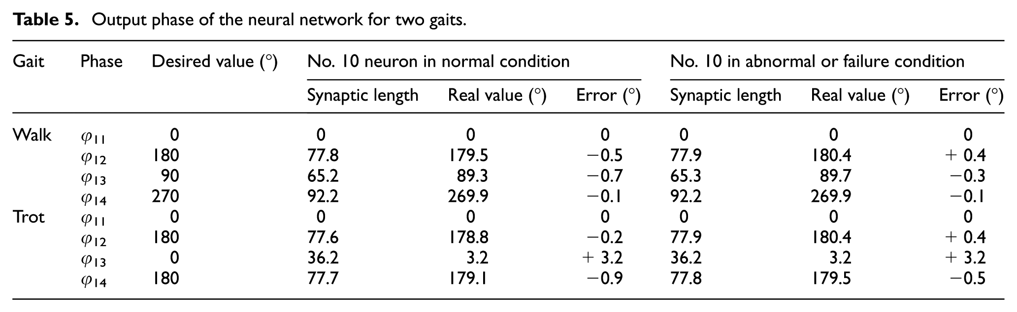
In Table 5, φ represents the phase difference and the subscript represents the output relationship between neurons. For example, φ₁₂ is the phase difference between the outputs of No. 1 neuron and No. 2 neuron.

Whether No. 10 neuron is normal or abnormal, there exists error between the actual phase difference of output neurons and expected phase difference. The error is within the allowable range of ±5°. Hence, the growth simulations shown in Figure 17 verify that the growing algorithm of neural network is effective. It can realize the growth process from the axon’s self-growth of single neuron to the harmonious growth of neural network.

The motion sequences of quadruped robot are given in Figure 18(a) through the simulations in the above two gaits. The movement periods of the walk gait and the tort gait are 1.2 and 0.6 s, respectively. Meanwhile, the change in the angular displacement α of the hip joint is tested and illustrated in Figure 18(b).

Figure 18.

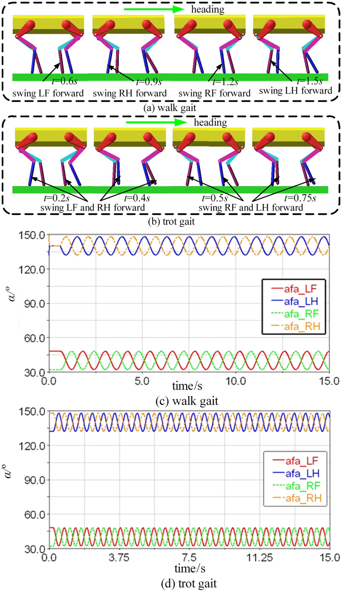
Simulation results of quadruped robot motions: (a) movement sequences, (b) angular displacement curves of hip joints, (c) walk gait, and (d) trot gait.

In Figure 18(c) and (d), the symbol “afa” represents the angle α of hip joint, and LF, LH, RF, and RH have the same meaning as previously defined in Figure 15. As can be seen from the illustration, the phase difference between hip joints of LF leg and LH leg is about 270° when the quadruped robot is walking. The phase differences from the hip joint of LF leg to that of RF leg and that of RH leg are 90° and 180°&0x44; respectively. When the quadruped robot is trotting, the hip joint of LF leg has almost the same phase with the hip joint of RF leg. The similar relationship also exists between the hip joint of LH leg and that of RH leg. The phase difference between the hip joint of LF leg and the hip joint of LH leg approximates to 90°. These results illustrate that the phases of joint angles for four hip joints meet the requirements in Table 5 when the quadruped robot walks or trots. And not only that, the phases hold constant and show obvious rhythmicity during the movements. The movement phase sequences of four legs of robot shown in Figure 18(b) are consistent with the descriptions in Figure 15. It means that our growing algorithm of neural network, compared to other similar algorithm, can effectively control the rhythmic movement of quadruped robot in walk gait and in trot gait.

Conclusion

This article has presented a growing algorithm of neural network based on axon self-growing model. The axon self-growing model was established using Newtonian gravitation and Brownian motion first. Compared with existing research results, the rationality of the model is verified. Then, the constraint function of axon growth was proposed by the gravitational coefficient and the Brownian coefficient. Combining the output function of neural network, the growing algorithm of neural network was developed. Finally, to verify the effectiveness of developed growing algorithm, simulations for the growth of neural network and the rhythmic motion control of quadruped robot in walk gait and in trot gait were performed, respectively. Simulation results show that the developed growing algorithm of neural network is reasonable, and the rhythmic motion of quadruped robot can be controlled effectively using this algorithm.

Footnotes

Handling Editor: Chenguang Yang

Declaration of conflicting interests

The author(s) declared no potential conflicts of interest with respect to the research, authorship, and/or publication of this article.

Funding

The author(s) disclosed receipt of the following financial support for the research, authorship, and/or publication of this article: This work was supported in part by the National Natural Science Foundation of China (Grant Nos 61773139 and 61473105); the Natural Science Foundation of Heilongjiang Province, China (Grant No. F2015008); State Key Laboratory of Robotics and System (HIT) (No. SKLRS201603C); the Shenzhen Peacock Plan (No. KQTD2016112515134654); and the Natural Science Foundation of Beijing and Shenzhen (No. U1713222).

ORCID iD

Pengfei Wang

References

Georgios

Gunnar

. On the application of self-growing networks for capacity and energy-saving improvements. In: Proceedings of the 2012 IEEE 17th international workshop on computer aided modeling and design of communication links and networks (CAMAD), Barcelona, 17–19 September 2012, pp.251–255. New York: IEEE.

Alonistioti

Merentitis

Schulz

et al . Towards self-adaptable, scalable, dependable and energy efficient networks: the self-growing concept. In: Proceedings of the 2010—the fourth international conference on mobile ubiquitous computing. systems, services and technologies, Florence, 25–30 October 2010, pp.324–327. Belgium: UGent.

Stephen

. A brief history of neuronal reconstruction. Neuroinformatics 2011; 9: 119–128.

Lowery

Vactor

. The trip of the tip: understanding the growth cone machinery. Nat Rev Mol Cell Biol 2009; 10: 332–343.

McLean

Arjen

Graham

. Continuum model for tubulin-driven neurite elongation. Neurocomputing 2004; 58–60: 511–516.

Johannes

Arjen

. A mathematical framework for modeling axon guidance. Bull Math Biol 2007; 69: 3–31.

Randal

Betty

Peter

et al . NETMORPH: a framework for the stochastic generation of large scale neuronal networks with realistic neuron morphologies. Neuroinformatics 2009; 7: 195–210.

Zubler

Douglas

. Framework for modeling the growth and development of neurons and networks. Front Comput Neurosci 2009; 3: 1–16.

Pearson

Emilio

Tara

et al . Mathematical modeling of axonal formation. Part I: geometry. Bull Math Biol 2011; 73: 2837–2864.

10.

Kobayashi

Terajima

Nozumi

et al . A stochastic model of neuronal growth cone guidance regulated by multiple sensors. J Theor Biol 2010; 26: 712–722.

11.

Aletti

Causin

. Mathematical characterisation of the transduction chain in growth cone pathfinding. IET Syst Biol 2008; 2: 150–161.

12.

Suter

Miller

. The emerging role of forces in axonal elongation. Prog Neurobiol 2011; 94: 91–101.

13.

Ponomarenko

. Linear superposition principle for partially coherent solitons. Phys Rev E Stat Nonlin Soft Matter Phys 2002; 65: 055601.

14.

Molina

Serna

Camacho

. Conditions of applicability of the superposition principle in potential multipulse techniques: implications in the study of microelectrodes. J Electroanal Chem 1995; 394: 1–6.

15.

Garbey

. On some applications of the superposition principle with Fourier basis. SIAM J Sci Comput 2000; 22: 1087–1116.

16.

Derek

Ekkehard

Jean

. On end-vertices of lexicographic breadth first searches. Discrete Appl Math 2010; 158: 434–443.

17.

Jiang

Wang

et al . Control of a quadruped robot with bionic springy legs in trotting gait. J Bionic Eng 2014; 11: 188–198.

18.

Johannes

Arjen

. A mathematical framework for modeling axon guidance. Bull Math Biol 2007; 69: 3–31.

19.

Zha

Guo

et al . Sodium ion channel optical model: depolarization spatial distribution and local potential dynamic spatiotemporal processes. Neurocomputing 2013; 99: 261–269.

20.

Zha

Wang

et al . Potassium ion channel optical model: membrane potential repolarization and its dynamic spread process. Neurocomputing 2013; 99: 316–324.

21.

Myriam

David

. Deletions of rhythmic motoneuron activity during fictive locomotion and scratch provide clues to the organization of the mammalian central pattern generator. J Neurophysiol 2005; 94: 1120–1132.

22.

Pérez

Tapia

Mirasso

et al . An intersegmental neuronal architecture for spinal wave propagation under deletions. J Neurosci 2009; 29: 10254–10263.

23.

Fei

Gao

Selvaggio

et al . A framework of teleoperated and stereo vision guided mobile manipulation for industrial automation. In: Proceedings of the IEEE international conference on mechatronics and automation, vol. 1641, Harbin, China, 7–10 August 2016. New York: IEEE.

24.

Qiu

et al . Teleoperation control of an exoskeleton robot using brain machine interface and visual compressive sensing. IEEE T Fuzzy Syst 2017; 25: 58–69.

25.

Yang

Wang

et al . Teleoperation control based on combination of wave variable and neural networks. IEEE T Syst Man Cy: S 2017; 47: 2125–2136.

26.

Yang

Luo

Pan

et al . Personalized variable gain control with tremor attenuation for robot teleoperation. IEEE T Syst Man Cy: S. Epub ahead of print 8 May 2017. DOI: 10.1109/TSMC.2017.2694020.

27.

Yang

Wang

Cheng

et al . Neural-learning-based telerobot control with guaranteed performance. IEEE T Cybernetics 2017; 47: 3148–3159.

28.

Wang

Guo

et al . CPG control for biped hopping robot in unpredictable environment. J Bionic Eng 2012; 9: 29–38.

29.

Martinez-Silva

Manjarrez

Gutierrez-Ospina

et al . Electrophysiological representation of scratching CPG activity in the cerebellum. PLoS ONE 2014; 9: e109936.

30.

Wang

Guo

et al . velocity control of a bounding quadruped via energy control and vestibular reflexes. J Bionic Eng 2014; 11: 556–571.

31.

Wang

et al . Bio-inspired controller for a robot cheetah with a neural mechanism controlling leg muscles. J Bionic Eng 2012; 9: 282–293.

A neural network growing algorithm based on Brownian movement and gravity constraint

Abstract

Keywords

Introduction

Self-growing model of neuron axon

Perception module

Motion module

Growth module

A growing algorithm of neural network

Growth constraint of the neuron axon

Connection algorithm of the neural network

Output function of the neural network

Parameter analysis

The time interval Δt and random rotation angle θs

The gravitational coefficient s

Experiment plot

Results and discussion

Conclusion

Footnotes

Declaration of conflicting interests

Funding

ORCID iD

References

The time interval Δt and random rotation angle θ_s