Sage Journals: Discover world-class research

Abstract

In this study, codimension-two bifurcation analysis was used in conjunction with a novel control method to mediate chaos in a semi-active suspension system based on a quarter-car model with excitation introduced by the road surface profile. The results of bifurcation analysis indicate that the hysteretic nonlinear characteristics of the damping forces produce codimension-two bifurcation, resulting in homoclinic orbits and pitchfork bifurcation. We also characterized the complex dynamics of vehicle suspension systems using a bifurcation diagram, phase portraits, Poincaré maps, and frequency spectra. Furthermore, the largest Lyapunov exponent was used to identify the onset of chaotic motion and to verify the results of bifurcation analysis. We also developed a continuous feedback control method based on synchronization characteristics to eliminate chaotic oscillations. Finally, we conducted analysis on the robustness of parametric perturbation in suspension systems with synchronization control using Lyapunov stability theory and numerical simulations.

Keywords

Codimension-two bifurcation chaos Lyapunov exponent synchronization

Introduction

Vehicle suspension systems are meant to isolate the body of the vehicle (and their occupants) from oscillations produced by a rough surface road profile. They are also meant to maintain continuous contact between wheels and the surface of the road. Ride comfort requires a long suspension stroke and low damping in wheel-hop mode.¹ The development of smart materials has prompted research into intelligent vehicle suspension systems featuring hysteretic damping characteristics based on electro-rheological fluid or magneto-rheological fluid.^2–5 The hysteretic nature of damping forces in vehicle suspension systems under excitation means that they can be modeled as a multi-frequency harmonic function. Thus, vehicle suspension can be simplified as a hysteretic nonlinear system with multi-frequency excitation.

Nonlinear codimension bifurcation has been studied extensively.^6–8 Farshidianfar and Saghafi⁹ studied global bifurcation behavior in spur gear systems. He et al.¹⁰ used the center manifold and normal form method to investigate codimension-two bifurcation behavior in a delayed neuron model. Tian et al.¹¹ examined the complex nonlinear dynamics associated with smooth, discontinuous oscillators. Vahdati and Kazemi¹² studied cascading period doubling bifurcations in periodic orbits emerging from Hopf bifurcations and chaos in power system. Ghosh et al.¹³ investigated chaos and bifurcation in a permanent magnet direct current (PMDC) brushed motor caused by slotting effects and commutation.

The characteristics of suspension systems with hysteretic damping are inherently nonlinear due to the fact that hysteresis is not a smooth process. This nonlinear behavior and inherent instability in this type of system complicate controller design. To predict or control the performance of a system with a reasonable degree of accuracy requires that the effects of nonlinear phenomena be taken into account. Modern nonlinear theories pertaining to bifurcation and chaos have been widely applied in the study of stability in nonlinear systems, and several studies have investigated nonlinear dynamics in suspension systems^14–17 as well as chaotic responses in nonlinear air suspension systems.^18,19

Despite extensive research into the dynamic characteristics of suspension systems, the issue of codimension bifurcations has yet to be fully elucidated. In this study, we consider codimension-two bifurcation and homoclinic orbits in this type of system. We adopted a variety of numerical analysis methods, including bifurcation diagrams, phase portraits, Poincaré maps, and frequency spectra, to explain the rich dynamic behavior of vehicle suspension systems excited by the road profile. We also employed the well-developed algorithms used to compute Lyapunov exponents for smooth dynamical systems²⁰ to determine whether the system exhibits chaotic motion. Chaotic behavior degrades performance and restricts the operating range of numerous electrical and mechanical devices. Since the pioneering work of Ott et al.,²¹ researchers have developed a number of technologies to mediate the effects of chaos in a range of applications, including suspension systems.^15,22–25

Improving the performance of a suspension system requires that chaotic motion be transformed into a steady-state periodic orbit. In this study, we developed a continuous feedback control method based on the properties of synchronization, as proposed by Pyragas²⁶ and Kapitaniak.²⁷ Simulation results demonstrate the efficacy of the proposed control mechanism. The design of the proposed feedback controller was validated through the application of optimal control and Lyapunov stability theories, which guarantee the global stability of a nonlinear error system.^28–30

Mathematical modeling

Figure 1 presents the quarter-car model with hysteretic nonlinear damping force with a single degree of freedom¹⁴ examined in this study

m \overset{\cdot\cdot}{x} + k_{1} (x - x_{0}) + F_{h} = 0

(1)

where F_h is an additional nonlinear hysteretic suspension damping and stiffness force that depends on relative displacement and velocity, as follows

F_{h} = k_{2} {(x - x_{0})}^{3} + C_{1} (\overset{\cdot}{x} - {\overset{\cdot}{x}}_{0}) + C_{2} {(\overset{\cdot}{x} - {\overset{\cdot}{x}}_{0})}^{3}

(2)

and

x_{0} = \tilde{a} \sin (Ω t)

(3)

Figure 1.

Schematic diagram of the quarter-car model.

By defining a new variable for the relative displacement, y = x−x₀, we can rewrite equation (1) as follows

\overset{\cdot\cdot}{y} + ω^{2} y + B_{1} y^{3} + B_{2} \overset{\cdot}{y} + B_{3} {\overset{\cdot}{y}}^{3} = A \sin (Ω t)

(4)

where $ω^{2} = k_{1} / m$ , $B_{1} = k_{2} / m$ , $B_{2} = C_{1} / m$ , $B_{3} = C_{2} / m$ , and $A = \tilde{a} Ω^{2}$ .

The states are selected such that $y_{1} = y, y_{2} = \overset{\cdot}{y}$ . Equation (4) is then transformed into the following state space equations

{\overset{\cdot}{y}}_{1} = y_{2}

(5a)

{\overset{\cdot}{y}}_{2} = - ω^{2} y_{1} - B_{1} {y_{1}}^{3} - B_{2} y_{2} - B_{3} {y_{2}}^{3} + A \sin (Ω t)

(5b)

The amplitude of road profile excitation is $\tilde{a} = 0$ . Table 1 presents the values of the parameters in the above equations obtained using the methods outlined by Li et al.¹⁴

Table 1.

Nomenclature and parameters.

Notation	Value	Unit	Description
m	240	kg	The body mass
k ₁	16 × 10⁴	N/m	The suspension stiffness coefficient
k ₂	30 × 10⁴	N/m³	The nonlinear hysteretic suspension stiffness coefficient
C ₁	250	Ns/m	The linear damping coefficient
C ₂	−25	Ns³/m³	The nonlinear hysteretic suspension viscous damping coefficient
$\tilde{a}$	0.05	m	The amplitude of road excitation
x ₀		m	The road excitation
x		m	The body’s vertical displacement
Ω		rad/s	The frequency of road excitation

Codimension-two bifurcation analysis

Our main objective in this analysis was to observe the qualitative behavior of a suspension system and determine how it varies with changes in system parameters. Changes were shown to occur near the equilibrium point of the system, which is referred to as local bifurcation. The codimension of a bifurcation is the minimum number of parameters that must be varied in order to observe a specific type of bifurcation.⁸

All nonlinear analyses must be based on linear analysis. Thus, bifurcation analysis begins with the Jacobian matrix of equation (5). Using parameters (k₁,c₁) = (0,0), the Jacobian matrix has double-zero eigenvalues, which is the most degenerate situation (eigenvalues with zero real parts). This is the well-known codimension-two bifurcation problem. The bifurcation equations are written as follows

{\overset{\cdot}{y}}_{1} = y_{2}

(6a)

{\overset{\cdot}{y}}_{2} = - B_{1} {y_{1}}^{3} + higher order terms

(6b)

These bifurcation equations take the normal form, which is the simplest form for equations of motion.^8,31–34

We adopted the blow-up technique to determine whether the cubic terms in equation (6) determine local behavior. The blow-up technique involves changing singular coordinates to expand degenerate fixed points into circles containing a finite number of fixed points. In cases where the fixed points are hyperbolic after the coordinate change, local flow near the circle is stable with respect to higher order terms (h.o.t.). This means that the flow near the original fixed point is also stable. If all of these fixed points are degenerate, then the coordinates must be changed again. If all of the fixed points become hyperbolic within a finite number of coordinate changes, then a system with only lower order terms will present the same qualitative behavior as the system as a whole.⁸ The steps used in the blow-up method are as follows

y_{1} = r \cos θ

(7a)

(first blow-up)

y_{2} = r \sin θ

(7b)

Equation (6) becomes

\overset{\cdot}{r} = r \sin θ \cos θ (1 - B_{1} r^{2} \cos^{2} θ) + h . o . t .

(8a)

\overset{\cdot}{θ} = - \sin^{2} θ - B_{1} r^{2} \cos^{4} θ + h . o . t .

(8b)

Stability analysis reveals that the system has two degenerate equilibrium points, (0,0) and (0,π). Therefore, the blow-up procedure must be repeated.

For (0,0), the power series in the normal form is written as follows

\overset{\cdot}{r} = r θ + h . o . t .

(9a)

\overset{\cdot}{θ} = - θ^{2} - B_{1} r^{2} + h . o . t .

(9b)

Let

r = ρ \sin ϕ

(10a)

(second blow-up)

θ = ρ \cos ϕ

(10b)

such that equation (9) becomes

\overset{\cdot}{ρ} = - ρ^{2} \cos ϕ (B_{1} \sin^{2} ϕ + \cos^{2} ϕ - \sin^{2} ϕ) + h . o . t .

(11a)

\overset{\cdot}{ϕ} = ρ \sin ϕ (2 \cos^{2} ϕ + B_{1} \sin^{2} ϕ) + h . o . t .

(11b)

After dividing by the unaffected common component ρ, equation (11) produces two hyperbolic fixed points (0,0) and (0,π). Therefore, no more blow-up is required.

For the other equilibrium point (0,π), the power series in the normal form is the same as in equation (9); therefore, the same results are obtained. The degenerate field contains cubic terms of the lowest order and unfolding is performed using the two-parameter family

{\overset{\cdot}{y}}_{1} = y_{2}

(12a)

{\overset{\cdot}{y}}_{2} = K_{1} y_{1} + K_{2} y_{2} - B_{1} {y_{1}}^{3}

(12b)

where $K_{1} = - k_{1} / m, K_{2} = - c_{1} / m$ . In equation (12), the h.o.t. are disregarded such that this form is used instead of the original equation (5).

The bifurcation set is the set in the parameter space on which the system bifurcates. It is obtained from the unfolded normal form equations.

There are three equilibrium points in this case:

(0,0) for all K₁, K₂;

$(\pm \sqrt{\frac{K_{1}}{B_{1}}}, 0)$ for K₁ > 0.

By determining the stability of these equilibria, the bifurcation sets can be obtained as follows:

1. For K₁ = 0

There is a subcritical pitchfork bifurcation if K₂ > 0 and a supercritical pitchfork bifurcation if K₂ < 0.

2. For K₁ > 0 and K₂ = 0

The rescaling technique and Melnikov’s perturbation method⁸ are used to obtain the complete bifurcation set associated with homoclinic orbits for the unfolding bifurcation in equation (12).

Let $y_{1} = ϵ u$ , $y_{2} = ϵ^{2} v$ , $K_{1} = ϵ^{2} v_{1}$ , $K_{2} = ϵ^{3} v_{2}$ , and $t \to ϵ t$ . Once it has been rescaled, equation (12) becomes

\overset{\cdot}{u} = v

(13a)

\overset{\cdot}{v} = v_{1} u + ϵ^{2} v v_{2} - B_{1} u^{3}

(13b)

Melnikov’s method is then used to characterize the approximate relationship between K₁ and K₂.

After a series of operations, the following expression is obtained

K_{2} = 0

(14a)

K_{1} = B_{1} ϵ^{3}

(14b)

Equation (14) yields a homoclinic saddle connection referred to as homoclinic bifurcation

3. For K₁ < 0 and K₂ = 0

The Jacobian matrix in equation (12) is written as

DF (0, 0) = [\begin{matrix} 0 & 1 \\ K_{1} & 0 \end{matrix}]

(15)

and the eigenvalues of DF(0,0) are

λ = \pm \sqrt{K_{1}} i

(16)

For changes in coordinates

[\begin{matrix} y_{1} \\ y_{2} \end{matrix}] = [\begin{matrix} 0 & 0 \\ - \sqrt{K_{1}} & 0 \end{matrix}] [\begin{matrix} U \\ V \end{matrix}]

(17)

Equation (12) then becomes

[\begin{matrix} \overset{\cdot}{U} \\ \overset{\cdot}{V} \end{matrix}] = [\begin{matrix} K_{2} & - \sqrt{K_{1}} \\ \sqrt{K_{1}} & 0 \end{matrix}] [\begin{matrix} U \\ V \end{matrix}] + [\begin{matrix} 0 \\ \frac{B_{1} V^{3}}{\sqrt{K_{1}}} \end{matrix}]

(18)

Let $g (U, V) = B_{1} V^{3} / \sqrt{K_{1}}$ and $f (U, V) = 0$ , such that we derive the following

\begin{matrix} f_{vvv} = 0, f_{vuu} = 0 \\ g_{vvu} = 0, g_{uuu} = 0 \\ f_{uu} = 0, f_{uv} = 0, f_{vv} = 0 \\ g_{uu} = 0, g_{uv} = 0, g_{vv} = 0 \end{matrix}

According to the Hopf bifurcation theorem,⁸ coefficient a cannot equal zero. In this case, equality with zero indicates that there is no Hopf bifurcation.

We performed numerical simulations using the original equation (5) to determine the validity of this bifurcation analysis. The parameter space was divided into several regions using bifurcation sets in Figure 2. We employed the commercial package DIVPRK of IMSL³⁵ using FORTRAN for mathematical subroutines to solve these ordinary differential equations. The resulting numerical simulations are presented in Figures 3 –7. The results for each parametric region are discussed below.

Figure 2.

Bifurcation sets associated with typical phase portraits in each region (P⁺: subcritical pitchfork, P⁻: supercritical pitchfork, SC: homoclinic bifurcation).

Figure 3.

Phase portrait for region (I) with (K₁,K₂) = (0.02,0.01).

Figure 4.

Phase portrait for SC with (K₁,K₂) = (0.02,0.0).

Figure 5.

Phase portrait for region (II) with (K₁,K₂) = (0.02,−0.01).

Figure 6.

Phase portrait for region (III) with (K₁,K₂) = (−0.02,−0.01).

Figure 7.

Phase portrait for region (V) with (K₁,K₂) = (−0.02,0.01).

Region (I) includes two sources and a saddle. Initial conditions in the neighborhood of the two sources are an indication that the mass is distant from the equilibrium points (Figure 3). At the boundary between regions (I) and (II) (i.e. in the bifurcation set SC (K₂ = 0, K₁ > 0)), the system is integrable with homoclinic orbits (Figure 4). Therefore, if we disregard the damping term, the system is conservative. In region (II), the system is not integrable, presenting two sinks and one saddle. If the initial conditions are in the neighborhood of the saddle, then the mass returns to the two sinks (i.e. stable points) as the time approaches infinity (see Figure 5). At the boundary between regions (II) and (III) (i.e. in bifurcation set P⁻), the two sinks move closer to the saddle as the parameters approach bifurcation set P⁻, and the region of stability shrinks to zero. In region (III), the two sinks disappear and saddle (0,0) becomes a sink. This is a supercritical pitchfork bifurcation with an attracting sink region (III) (Figure 6). From regions (III) to (V), the eigenvalues for the Jacobian matrix cross the imaginary axis; however, Hopf bifurcation does not occur. This is a demonstration of linear dynamic behavior, similar to the situation in which a stable equilibrium point becomes an unstable equilibrium point (Figure 7). Between regions (V) and (I), boundary P⁺ must be crossed via subcritical pitchfork bifurcation. In Figure 2, K₁ determines the number of equilibrium points and K₂ determines the local behavior (e.g. stability or instability) and the existence of homoclinic orbits. Clearly, only a positive damping coefficient results in a stable system.

Analytical tools for observing overall characteristics of a vehicle suspension system

In equation (4), the amplitude of road excitation, $\tilde{a}$ , equals 0.05 m. We performed a series of numerical simulations using equation (5) to elucidate the characteristics of this system. Rich dynamics can be better observed when a range of parameter values are employed in a bifurcation diagram. This type of diagram is widely used to describe transitions from periodic to chaotic motion in dynamic systems. The resulting bifurcation diagram in Figure 8 clearly shows the existence of chaotic motion in region A. Period-one motion appears in region C, which includes a stable equilibrium point. Herein, each response is characterized using a phase portrait, a Poincaré map (velocity vs. phase angle), and a frequency spectrum. Figure 9 indicates that the equilibrium point of the system will remain stable as long as the parameter Ω exists in region C. When the parameter Ω exists in region B, we observe quasi-periodic motion in this region. When Ω = 7.98, 8.07, or 8.17, the system exhibits quasi-periodic motion and the map forms a continuous closed orbit in the Poincaré section. As shown in Figures 10 –12, a quasi-periodic trajectory is restricted to an annular-like region in the state space and differs considerably from periodic trajectories. As shown in Figure 13, when the forcing frequency (Ω) decreases into region A, chaotic motion produces chatter vibration. The transition sequence for the system is from periodic motion to quasi-periodic motion, and finally to chaotic motion. The features specific to these two descriptors characterize the chaotic behavior. The Poincaré map contains an infinite set of points referred to as a strange attractor. The frequency spectrum for chaotic motion is a continuous broad spectrum. These two features—the strange attractor and the continuous Fourier spectrum—are strong indicators of chaos. Figure 13 clearly shows chaotic behaviors in region A. Figure 13(a)–(c) presents the phase portraits, Poincaré maps, and frequency spectra, respectively.

Figure 8.

Bifurcation diagram showing the amplitude of road excitation $\tilde{a} = 0.05 m$ .

Figure 9.

Period-one orbit at Ω = 8.25 rad/s: (a) phase portrait, (b) Poincaré map, and (c) frequency spectrum.

Figure 10.

Quasi-periodic orbit at Ω = 7.98 rad/s: (a) phase portrait, (b) Poincaré map, and (c) frequency spectrum.

Figure 11.

Quasi-periodic orbit at Ω = 8.07 rad/s: (a) phase portrait, (b) Poincaré map, and (c) frequency spectrum.

Figure 12.

Quasi-periodic orbit at Ω = 8.17 rad/s: (a) phase portrait, (b) Poincaré map, and (c) frequency spectrum.

Figure 13.

Chaotic motion at Ω = 7.964 rad/s: (a) phase portrait, (b) Poincaré map, and (c) frequency spectrum.

Analysis of chaotic behavior

Our analysis in section 4, cannot be used to identify chaotic motion in a suspension system. Thus, in this section, we use Lyapunov exponents to verify the occurrence of chaotic motion. In every dynamic system, a spectrum of Lyapunov exponents (λ)²⁰ indicates variations in the length, area, and volume of a phase space. Determining whether chaos exist requires only the calculation of the largest Lyapunov exponent, which indicates whether the nearby trajectories diverge (λ > 0) or converge (λ < 0), on average. Any bounded motion within a system with at least one positive Lyapunov exponent is defined as chaotic, whereas periodic motion requires that all Lyapunov exponents be nonpositive.

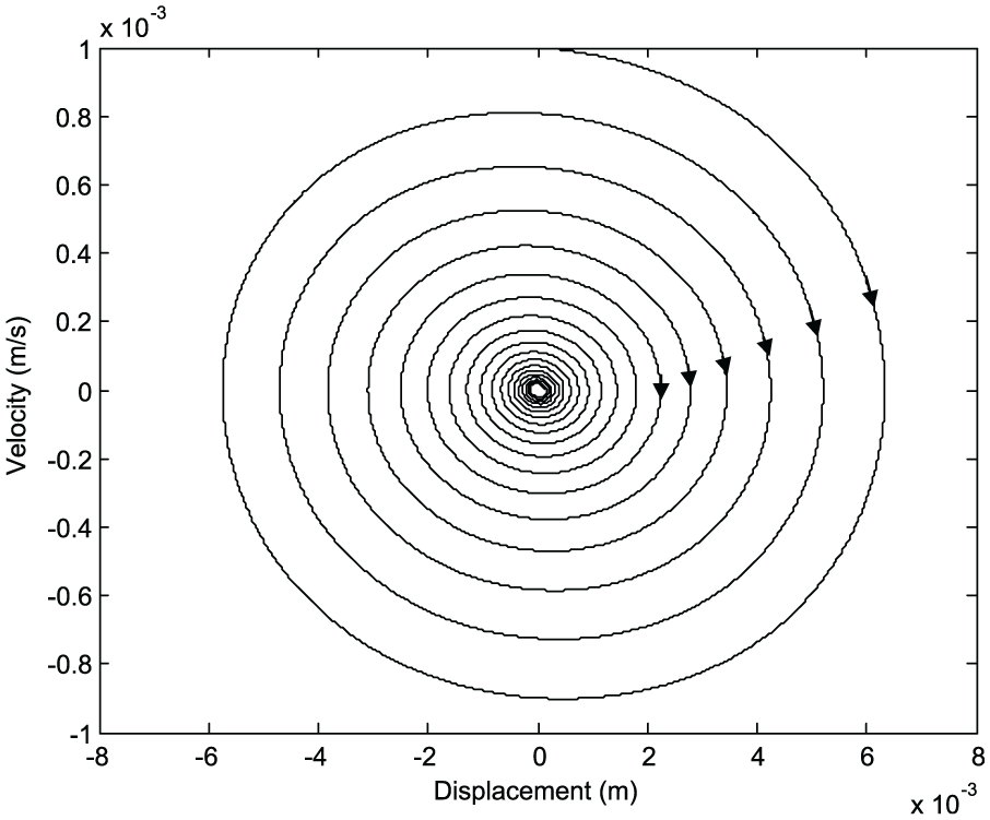
As shown in Figure 14, we computed the evolution of the largest Lyapunov exponent in the suspension system using the algorithm proposed by Wolf et al.²⁰ Figure 14 reveals the onset of chaotic motion at approximately Ω = 7.965 rad/s, that is, at point P₁ where the sign of the largest Lyapunov exponent changes from negative to positive as the parameter Ω is slowly decreased. Between the points P₁ and P₂, the largest Lyapunov exponent approaches zero, such that the motion within the system is denoted as quasi-periodic. When the value of Ω exceeds P₁ (e.g. when Ω = 8.25 rad/s), the Lyapunov exponents given by equation (5) are λ₁ = −0.0297643 and λ₂ = −0.0298612. The fact that the sum of these values (λ₁ + λ₂ = −0.0596255) is negative indicates that the motion of mass would eventually converge to a stable limit cycle. Using the Lyapunov exponents for a dynamic system with $λ_{1} \geq \dots \geq λ_{n}$ , Kaplan and Yorke³⁶ estimated the Lyapunov dimension, d_L, as follows

d_{L} = j + \frac{1}{| λ_{j + 1} |} \sum_{i = 1}^{j} λ_{i}

(19)

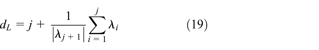
where j is the largest integer that satisfies $\sum_{i = 1}^{j} λ_{i} > 0$ . This technique yields a Lyapunov dimension of equation (5) for Ω = 8.25 rad/s, which is d_L = 1. The fact that the Lyapunov dimension is an integer indicates that the system exhibits periodic motion. When the parameter Ω increases beyond the bifurcation point (e.g. when Ω = 7.9638 rad/s), the Lyapunov exponents are λ₁ = 0.002269 and λ₂ = −0.0876695, and the Lyapunov dimension is d_L = 1.02588. In this case, the Lyapunov dimension is not an integer, which is an indication of chaotic motion. The Lyapunov dimension must be an integer for a periodic solution; however, it does not have to be an integer for a strange attractor.

Figure 14.

Evolution of the largest Lyapunov exponent.

Chaos synchronization

Learning to predict the behavior of a chaotic system has a number of benefits; however, the ultimate objective is to assume control over the system. Improving the performance of a dynamic system requires that the chaotic behavior be converted into stable periodic motion. Suitable control methods must therefore be developed. The chaos control method proposed by Ott, Grebogi, and Yorke (OGY)²¹ has been used to synchronize chaotic systems. The OGY method requires that the state of the system be continuously monitored using computer and Poincaré map to evaluate changes in the parameters. Corrections to the control parameters are slight and infrequent, such that fluctuating noise leads to occasional bursts into regions far from the desired orbits, which produces breaks in control or synchronization. To avoid these problems, Pyragas²⁶ and Kapitaniak²⁷ proposed a simple yet effective time-continuous control method by which to convert chaotic motion into periodic motion. This method involves the construction of a feedback mechanism in conjunction with a specific time-continuous perturbation. Figure 15 displays the proposed feedback control loop with external periodic perturbation. The proposed method is outlined briefly in the following.

Figure 15.

Block diagram of the proposed continuous chaos control method.

Consider the following n-dimensional dynamic system

\overset{\cdot}{x} = P (x) + F (t)

(20)

\overset{\cdot}{y} = Q (y)

(21)

where $x (t), y (t) \in R^{n}$ is the state vector and $F (t)$ is the input signal. Equation (20) without input signal (F(t) = 0) is assumed to have a strange attractor, whereas equation (21) displays periodic motion. A periodic system is usually referred to as the drive system, whereas a chaotic system is referred to as the response system. These two systems can be synchronized using the strategy outlined in Figure 15. The difference between the signal y(t) and the signal x(t) is used as a control signal as follows

F (t) = K [x (t) - y (t)]

(22)

which is introduced into the chaotic system (20) as negative feedback. In equation (22), K represents the feedback gain.

When Ω₁ = 8.25 rad/s is selected as the drive system, equation (5) reveals period-one motion

{\overset{\cdot}{y}}_{1} = y_{2}

(23a)

{\overset{\cdot}{y}}_{2} = - ω^{2} y_{1} - B_{1} {y_{1}}^{3} - B_{2} y_{2} - B_{3} {y_{2}}^{3} + A \sin (Ω_{1} t)

(23b)

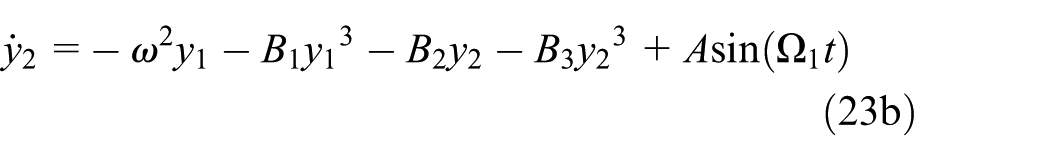
When Ω₂ = 7.964 rad/s is selected as the response system, equation (5) reveals chaotic motion

{\overset{\cdot}{x}}_{1} = x_{2}

(24a)

{\overset{\cdot}{x}}_{2} = - ω^{2} x_{1} - B_{1} {x_{1}}^{3} - B_{2} x_{2} - B_{3} {x_{2}}^{3} + A \sin (Ω_{2} t)

(24b)

To synchronize equations (23) and (24), we introduce into equation (24) a control signal in the form of equation (22).

When incorporated into equation (24), the control signal equation (22) yields the following coupled system, which is capable of achieving synchronization

{\overset{\cdot}{x}}_{1} = x_{2} + K (x_{1} - y_{1})

(25a)

\begin{array}{l} {\dot{x}}_{2} = - ω^{2} x_{1} - B_{1} {x_{1}}^{3} - B_{2} x_{2} \\ - B_{3} {x_{2}}^{3} + A \sin (Ω_{2} t) + K (x_{2} - y_{2}) \end{array}

(25b)

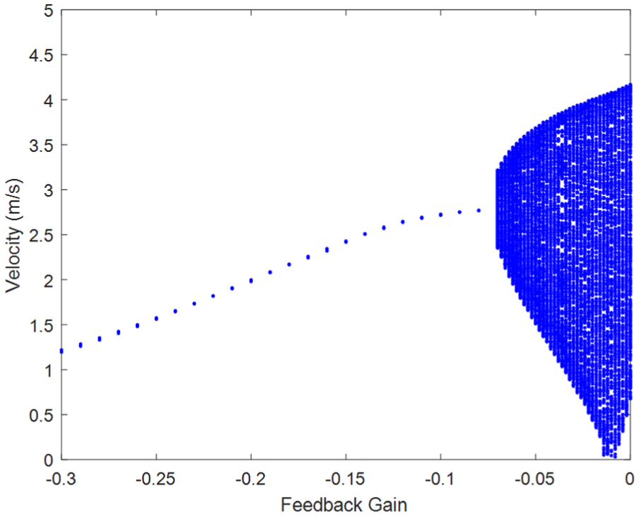
Equation (25) reveals chaotic motion (Figure 13) when K = 0 and Ω₂ = 7.964 rad/s. The feedback gain K was adjusted to be between 0.0 and −0.3 in order to convert the dynamics of the system (25) from chaotic motion into periodic motion. Figure 16 presents the resulting bifurcation diagram, which comprehensively explains the dynamic behavior over a range of feedback gains. Chaotic motion appeared when −0.075 < K ≤ 0 (with and without the control algorithm) and periodic motion appeared when K ≤ −0.075. Accordingly, if chaotic motion were converted into periodic motion, then the feedback gain would be selected to satisfy the condition K ≤ −0.075. The chaotic suspension system in equation (24) can be synchronized by applying a control signal with K = −0.1, as shown in Figure 17. This means that chaos in the system can be managed using the control signal (K = −0.1), thereby enabling the conversion of chaotic motion into a period-one orbit. In Figure 17(a), the dotted line denotes the time response of the suspension system without a control signal, whereas the solid line denotes the time response of the suspension system with a control signal. Figure 17(b) shows the plot of a phase portrait of the system to which the control signal was added.

Figure 16.

Bifurcation diagram of the system with continuous control, where K denotes the feedback gain.

Figure 17.

Chaotic motion controlled to the desired stable equilibrium point for K = −0.1 and Ω = 7.964 rad/s: (a) time responses of displacement, where dotted line represents the chaotic trajectory of the uncontrolled system and solid line represents the corresponding stable orbit of the controlled system; (b) phase portrait of the controlled system.

Effects of parametric perturbation on suspension system when using synchronization control

We consider the effects of parameter errors on the performance of the proposed controller by implementing synchronization control of chaos through the addition of a sinusoidal perturbation to parameters ω, B₁, B₂, and B₃ in the periodic excitation (drive system) in equation (23). Under the assumption that equation (23) represents the drive system, the corresponding controlled response system can be represented as follows

\frac{d z_{1}}{dt} = z_{2} + u_{1}

(26a)

\begin{array}{l} \frac{d z_{2}}{d t} = - ω^{2} {(1 + ε \sin \tilde{ω} t)}^{2} z_{1} - B_{1} (1 + ε \sin \tilde{ω} t) {z_{1}}^{3} \\ - B_{2} (1 + ε \sin \tilde{ω} t) z_{2} - B_{3} (1 + ε \sin \tilde{ω} t) {z_{2}}^{3} \\ + A \sin (Ω_{1} t) + u_{2} \end{array}

(26b)

where ε is the amplitude of the perturbation and $\tilde{ω}$ is the angular frequency.

Subtracting equation (23) from equation (26), we obtain the following error equation

\frac{d e_{1}}{dt} = e_{2} + u_{1}

(27a)

\begin{array}{l} \frac{d e_{2}}{d t} = - ω^{2} {(ε \sin \tilde{ω} t)}^{2} e_{1} - B_{1} ε \sin \tilde{ω} t {e_{1}}^{3} \\ - B_{2} ε \sin \tilde{ω} t e_{2} - B_{3} ε \sin \tilde{ω} t {e_{2}}^{3} + u_{2} \end{array}

(27b)

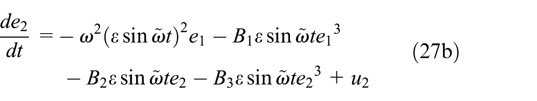
where $e_{1} = z_{1} - x_{1}$ and $e_{2} = z_{2} - x_{2}$

Considering a Lyapunov function for equation (27)

V (e) = \frac{1}{2} e^{T} e

(28)

We obtain the first derivative of V(e) as follows

\overset{\cdot}{V} (e) = e_{1} {\overset{\cdot}{e}}_{1} + e_{2} {\overset{\cdot}{e}}_{2}

(29)

Therefore, if we select

u_{1} = - e_{1} - e_{2}

(30a)

\begin{array}{l} u_{2} = - e_{2} + ω^{2} {(ε \sin \tilde{ω} t)}^{2} e_{1} + B_{1} ε \sin \tilde{ω} t {e_{1}}^{3} \\ + B_{2} ε \sin \tilde{ω} t e_{2} + B_{3} ε \sin \tilde{ω} t {e_{2}}^{3} \end{array}

(30b)

then

\overset{\cdot}{V} (e) = - e_{1}^{2} - e_{2}^{2}

(31)

$\overset{\cdot}{V} (e) < 0$ is satisfied. $\overset{\cdot}{V} (e)$ is a negative-defined function; therefore, the error states are $\lim_{t \to \infty} e (t) = 0$ . This means that the states of the controlled response system and the drive system are synchronized globally and asymptotically.³⁷

The correctness of these theoretical results was evaluated by performing simulations using the following perturbed parameters: ε = 0.05 and ω = 125.6 rad/s. Results of these simulations are presented in Figure 18(a) and (b). Figure 18(a) shows that e₁ = z₁ − x₁ and Figure 18(b) shows that e₂ = z₂ − x₂. These figures indicate that the synchronization error eventually converges to zero, resulting in stabilization of the error system. This implies that even in the face of parametric perturbations the controller is able to synchronize the states of the drive and response systems. This means that the proposed control method is robust to the effects of parameter mismatch in the suspension system. Finally, we use a bifurcation diagram to demonstrate the effects of parametric perturbations. The bifurcation diagram in Figure (19) clearly shows that the proposed control method is able to suppress the chaotic behavior under perturbed parameters (e.g. ω, B₁, B₂, and B₃) in periodic excitation using equation (23).

Figure 18.

Dynamics of synchronization errors for the drive system and the response system: (a) e₁ = z₁ − x₁ and (b) e₂ = z₂ − x₂.

Figure 19.

Bifurcation diagram of the controlled system with synchronization under perturbed parameters: $ω + ω ε \sin \tilde{ω} t$ , $B_{1} + B_{1} ε \sin \tilde{ω} t$ , $B_{2} + B_{2} ε \sin \tilde{ω} t$ , and $B_{3} + B_{3} ε \sin \tilde{ω} t$ .

Conclusion

This study focused on rich nonlinear dynamic behaviors in a vehicle suspension system with hysteretic damping. Our objective was to develop a method by which to control chaotic vibration. Dynamic behaviors can be observed over the entire range of parameter values of the bifurcation sets and bifurcation diagram. Bifurcation analysis was used to identify a codimension-two bifurcation structure with double-zero degeneracy in the system. The resulting bifurcation diagram indicates the existence of a quasi-periodic orbit and chaotic motion in the suspension system, thereby demonstrating the effectiveness of using the Lyapunov exponent as a tool for identifying chaotic motion. We developed a continuous feedback control method based on the properties of synchronization to suppress chaotic motion and thereby improve the ride of vehicles. The suspension system with synchronization control was analyzed in terms of robustness against parametric perturbation using Lyapunov stability theory and bifurcation diagram. The proposed synchronization control method does not require the monitoring of chaotic trajectories or the application of targeting procedures. The continuous nature of the synchronization-based control system makes it resistant to noise and facilitates application in actual vehicle systems. Simulation results confirm the feasibility of the proposed method. Our results provide insight into the operating conditions under which undesirable dynamic motion takes place in vehicle suspension systems. Our results also provide useful reference for engineers tasked with the design of control systems for vehicle suspension. The system considered in this article models an experimental vehicle suspension system, which could be used in subsequent investigations. Figure 20 presents a schematic depiction of the instrumentation used in the experimental study. A function generator supplied a sinusoidal signal. Waveform analysis in the time domain is made possible using an HP 3562A dynamic signal analyzer. The input signal of the controller includes the displacement, x, of the vehicle suspension system used in the experiments. A control signal is introduced into the chaotic system as a feedback control to synchronize the periodic signal with the chaotic system.

Figure 20.

Experimental set-up.

Footnotes

Handling Editor: Yong Chen

Declaration of conflicting interests

The author(s) declared no potential conflicts of interest with respect to the research, authorship, and/or publication of this article.

Funding

The author(s) disclosed receipt of the following financial support for the research, authorship, and/or publication of this article: This research was supported by the Ministry of Science and Technology in Taiwan, Republic of China, under project number MOST 105-2221-E-212-016.

References

Chen

Liu

Sun

. Application of constrained H_∞ control to active suspension systems on half-car models. J Dyn Sys Meas 2005; 127: 345–354.

Song

Ahmadian

Southward

et al . Parametric study of nonlinear adaptive control algorithm with magneto-rheological suspension systems. Commun Nonlinear Sci 2007; 12: 584–607.

Gui

Shi

Liu

. A semi-active suspension design for off-road vehicle base on magneto-rheological technology. In: Proceedings of the 9th international conference on fuzzy systems and knowledge discovery (FSKD), Sichuan, China, 29–31 May 2012. New York: IEEE.

Yang

et al . Experimental study and design on automobile suspension made of magneto-rheological damper. Energy Proced 2012; 16: 417–425.

Nugroho

et al . Implementation of adaptive neuro fuzzy inference system controller on magneto rheological damper suspension. In: Proceedings of the IEEE/ASME international conference on advanced intelligent mechatronics (AIM), Wollongong, NSW, Australia, 9–12 July 2013. New York: IEEE.

Arnold

. Geometrical methods in the theory of ordinary differential equations. New York: Springer, 1988.

Holmes

. Bifurcation to divergence and flutter in flow induced oscillations: a finite dimensional analysis. J Sound Vib 1977; 53: 471–503.

Guckenheimer

Holmes

. Nonlinear oscillations, dynamical system and bifurcation of vector fields. New York: Springer, 2013.

Farshidianfar

Saghafi

. Global bifurcation and chaos analysis in nonlinear vibration of spur gear systems. Nonlinear Dynam 2014; 75: 783–806.

10.

Huang

et al . Codimension two bifurcation in a simple delayed neuron model. Neural Comput Appl 2013; 23: 2295–2300.

11.

Tian

Cao

Yang

. The codimension-two bifurcation for the recent proposed SD oscillator. Nonlinear Dynam 2010; 59: 19–27.

12.

Vahdati

Kazemi

. Bifurcations and chaos in nonlinear dynamics of power systems. In: Proceedings of the IEEE conferences 24th Iranian conference on electrical engineering (ICEE), Shiraz, Iran, 10–12 May 2016. New York: IEEE.

13.

Ghosh

Panda

Saha

. Analysis of chaos and bifurcation due to slotting effect and commutation in a current discontinuous permanent magnet brushed DC motor drive. IEEE T Ind Electron 2018; 65: 2001–2008.

14.

Yang

Guo

. Investigation on chaotic motion in hysteretic non-linear suspension system with multi-frequency excitations. Mech Res Commun 2004; 31: 229–236.

15.

Naik

Singru

. Resonance, stability and chaotic vibration of a quarter-car vehicle model with time-delay feedback. Commun Nonlinear Sci 2011; 16: 3397–3410.

16.

Taffo

GIK

Siewe

. Parametric resonance, stability and heteroclinic bifurcation in a nonlinear oscillator with time-delay: application to a quarter-car model. Mech Res Commun 2013; 52: 1–10.

17.

Zhou

Song

Sun

et al . Nonlinear dynamic analysis of a quarter vehicle system with external periodic excitation. Int J Nonlin Mech 2016; 84: 82–93.

18.

Marzbanrad

Keshavarzi

. Chaotic vibrations of a nonlinear air suspension system under consecutive half sine speed bump. Ind J Sci Technol 2015; 8: 72–84.

19.

Marzbanrad

Keshavarzi

. A chaotic viewpoint on a quarter-car air suspension model with numerical and experimental analysis. J Cahiers Sci 2014; 23: 19–47.

20.

Wolf

Swift

Swinney

et al . Determining Lyapunov exponent from a time series. Physica D 1985; 16: 285–317.

21.

Ott

Grebogi

Yorke

. Controlling chaos. Phys Rev Lett 1990; 64: 1196–1199.

22.

Hunt

. Stabilizing high-period orbits in a chaotic system: the diode resonator. Phys Rev Lett 1990; 67: 1953–1955.

23.

Cai

et al . Notch filter feedback control in a class of chaotic systems. Automatica 2002; 38: 695–701.

24.

Litak

Borowiec

Ali

et al . Pulsive feedback control of a quarter car model forced by a road profile. Chaos Soliton Fract 2007; 33: 1672–1676.

25.

Sze

Lam

. Semi-active H control of vehicle suspension with magneto-rheological dampers. J Sound Vib 2005; 283: 981–996.

26.

Pyragas

. Continuous control of chaos by self-controlling feedback. Phys Lett A 1992; 170: 421–428.

27.

Kapitaniak

. Continuous control and synchronization in chaotic systems. Chaos Soliton Fract 1995; 6: 237–244.

28.

Rafikov

Balthazar

. On control and synchronization in chaotic and hyperchaotic systems via linear feedback control. Commun Nonlinear Sci 2008; 13: 1246–1255.

29.

Rafikov

Balthazar

Tusset

. An optimal linear control design for nonlinear systems. J Braz Soc Mech Sci Eng 2008; 30: 279–284.

30.

Nozaki

Balthazar

Tusset

et al . Nonlinear control system applied to atomic force microscope including parametric errors. J Control Autom Electr Syst 2013; 24: 223–231.

31.

Ashkenazi

Chow

. Normal forms near critical points for differential equations and maps. IEEE T Circuit Syst 1988; 35: 850–862.

32.

Bibikov

. Local theory on nonlinear analytic ordinary differential equations. New York: Springer, 1979.

33.

Chau

Kokubu

. Normal forms for nonlinear vector fields—part I: theory and algorithm. IEEE T Circuit Syst 1988; 35: 863–880.

34.

Holmes

. Dynamics of a nonlinear oscillator with feedback control I: local analysis. J Dyn Sys Meas 1985; 107: 159–165.

35.

IMSL. User’s Manual IMSL MATH/LIBRARY. Houston, TX: IMSL, 1989.

36.

Kaplan

York

. Chaotic behavior of multidimensional difference equations, lecture notes in mathematics. New York: Springer, 1979.

37.

Khalil

. Nonlinear systems. 3rd ed. Upper Saddle River, NJ: Prentice Hall, 2002.

Codimension-two bifurcation analysis and chaos synchronization of a quarter-car vehicle model

Abstract

Keywords

Introduction

Mathematical modeling

Codimension-two bifurcation analysis

Analytical tools for observing overall characteristics of a vehicle suspension system

Analysis of chaotic behavior

Chaos synchronization

Effects of parametric perturbation on suspension system when using synchronization control

Conclusion

Footnotes

Declaration of conflicting interests

Funding

References