Sage Journals: Discover world-class research

Abstract

A three-dimensional computational model of two CRH2 trains passing by each other in a tunnel was developed using finite volume method with moving mesh, to investigate the characteristics of air wave and flow field around high-speed trains. Two meeting scenarios (i.e. meeting at the same train speeds and at different train speeds) and five train speeds (i.e. 200, 250, 300, 350, and 400 km/h) were examined. The computational model is demonstrated to be qualified to investigate the characteristics of air wave for two trains meeting in a tunnel. The pressure distribution and velocity vectors of two trains meeting in a tunnel were revealed, and the typical features of the corresponding air wave curve were discussed. Furthermore, the variation regularity of pressure amplitudes and the relationship between pressure wave amplitude and train speed were also analyzed. The results indicate that two trains with a large speed difference should be avoided when they pass by each other in a tunnel. These findings are helpful to guide the design of trains and tunnel structures and the dispatching management of rail transit.

Keywords

High-speed train air wave numerical simulation meeting in a tunnel

Introduction

The propagation and characteristics of the air wave in a railway tunnel caused by the passage of a train or passing trains have increasingly aroused great academic and engineering concerns in rail transport.^1–5 With the increased speed of trains, the magnitude of the initial pressure rise generated around the car body becomes much larger than that in the open sections; this unsteady aerodynamic loading may destabilize the trains (i.e. the car body is in a state of sway and yawing motion), and thus cause larger running vibrations.^1,3 Furthermore, the generated air wave may cause appreciable aural discomfort to passengers. Especially at the exit of the tunnel, the air wave is emitted toward the surrounding area, and an extremely loud explosive sound occurs, resulting in a potential environmental low-frequency noise.^3,6–8 This problem gets more severe with increased train speed, attributed to the fact that the radiated noise energy is proportional to the power of the train speed.⁶

The air wave generated by a train passing through a tunnel is a complicated aerodynamic phenomenon of unsteady compressible flow. Numerous studies^9–11 have been conducted to predict the pressure transients in a tunnel based on one-dimensional (1D) unsteady compressible flow models. For long tunnels, the 1D flow assumption is reasonable and valid; however, for short tunnels, the simplifications of the train end as sharp discontinuities and the boundary conditions at the tunnel portals may greatly affect the computed results of pressure distributions. This is because the flow around the train contains large regions of recirculation, and the strength of the air wave propagating in the tunnel is not a constant over the cross section.³ Therefore, many three-dimensional (3D) considerations have been performed to investigate the compressible flow in a railway tunnel. Howe¹² developed a theory of pressure wave generation by trains passing in a tunnel, in terms of a Green’s function describing the interaction of a point source with a moving train, to calculate the pressure transients generated by two trains passing by each other. Yau and Cheng¹³ used a 3D computational fluid dynamics (CFD) model to study the pressure fluctuation caused by the passage of two electric motorized unit (EMU) trains through a tunnel, and the influences of pressure wave on the aural comfort of passengers and the stability of train were also examined. Subsequently, Ko et al.¹⁴ conducted a series of field measurements of aerodynamic pressures in tunnels induced by high-speed trains with a maximum operation speed of up to 300 km/h. Meng et al.¹⁵ built a 3D unsteady compressible turbulence model using CFD software to simulate the whole crossing process of high-speed trains in a tunnel, including the constant-speed and variable-speed conditions. It can be concluded from the above literature survey that the studies on the pressure wave generated by two high-speed trains passing by each other in a tunnel are still very limited, although considerable attention has been paid to the aerodynamic problems of a single high-speed train passing through a tunnel. Meanwhile, due to the optimized and tight time schedules, the safety operation speed of trains passing through a tunnel is expected to be as high as possible. Hence, the issues of two high-speed trains passing by each other in a tunnel need to be studied widely in-depth, so as to provide technical guidance for the design of trains and tunnel structures and the dispatching management of rail transit.

Consequently, a 3D simplified computational model of two CRH2 trains passing by each other in the tunnel was established using finite volume method (FVM) with moving grids, to explore the distribution of the flow field around trains and characteristics of air wave in this article.

Computational model

Considering two CRH2 EMU trains passing by each other in a tunnel, with train speeds ranging from 200 to 400 km/h, the airflow around trains is taken as the compressible, viscous, and unsteady turbulent flow with a high Reynolds number. The computational model was solved using the Fluent commercial software.

Governing equation of fluid dynamics

As stated above, the flow field around two trains passing by each other in a tunnel is the compressible, viscous, and unsteady turbulent field. The Reynolds-averaged Navier–Stokes (RANS) equations and standard k–ε two-equation model were used.^16–18 The RANS equations can be written in Cartesian tensor form as

\frac{\partial ρ}{\partial_{t}} + \frac{\partial}{\partial x_{i}} (ρ u_{i}) = 0

(1)

\begin{array}{l} \frac{\partial}{\partial t} (ρ u_{i}) + \frac{\partial}{\partial x_{j}} (ρ u_{i} u_{j}) = - \frac{\partial p}{\partial x_{i}} + \frac{\partial}{\partial x_{j}} \\ [μ (\frac{\partial u_{i}}{\partial x_{j}} + \frac{\partial u_{j}}{\partial x_{i}} - \frac{2}{3} δ_{i j} \frac{\partial u_{l}}{\partial x_{l}})] + \frac{\partial}{\partial x_{j}} (- ρ {\bar{u}}^{'}_{i} {\bar{u}}^{'}_{j}) \end{array}

(2)

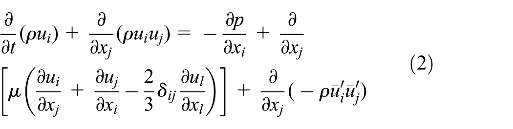
where ρ is the density of air; x_i, x_j, and x_l are the Cartesian coordinates, and u_i, u_j, and u_l are the corresponding fluid velocity components; p is the static pressure; δ_ij is a unit tensor; and $- ρ \bar{u}'_{i} \bar{u}'_{j}$ are the Reynolds stresses.

The turbulence kinetic energy, k, and its rate of dissipation, ε, are obtained from the following transport equations

\frac{\partial}{\partial t} (ρ k) + \frac{\partial}{\partial x_{i}} (ρ k u_{i}) = \frac{\partial}{\partial x_{j}} [(μ + \frac{μ_{t}}{σ_{k}}) \frac{\partial k}{\partial x_{j}}] + G_{k} - ρ ε + G_{b} - Y_{M} + S_{k}

(3)

and

\begin{array}{l} \frac{\partial}{\partial t} (ρ ε) + \frac{\partial}{\partial x_{i}} (ρ ε u_{i}) = \frac{\partial}{\partial x_{j}} [(μ + \frac{μ_{t}}{σ_{ε}}) \frac{\partial ε}{\partial x_{j}}] \\ + C_{1 ε} \frac{ε}{k} (G_{k} + C_{3 ε} G_{b}) - C_{2 ε} ρ \frac{ε^{2}}{k} + S_{ε} \end{array}

(4)

where G_k represents the generation of turbulence kinetic energy due to the mean velocity gradients; G_b is the generation of turbulence kinetic energy due to buoyancy; Y_M represents the contribution of the fluctuating dilatation in compressible turbulence to the overall dissipation rate; C_1ε, C_2ε, and C_3ε are constants; σ_k and σ_ε are the turbulent Prandtl numbers for k and ε, respectively; S_k and S_ε are the user-defined source terms; and µ_t is the turbulent viscosity, which is computed by combining k and ε as follows

μ_{t} = ρ C_{μ} \frac{k^{2}}{ε}

(5)

where C_µ is a constant. These model constants have been determined from experiments with air and water for fundament turbulent shear flows including homogeneous shear flows and decaying isotropic grid turbulence and given by C_1ε = 1.44, C_2ε = 1.92, C_µ = 0.09, σ_k = 1.0, and σ_ε = 1.3.¹⁶

Geometry modeling and computational domain

To balance the computational precision and efficiency, some reasonable simplifications for the computational model are made: (1) the train model is simplified into three-car marshaling including one head car, one middle car, and one tail car, where the head car and tail car have the same car appearance; (2) all the surfaces of the train are considered to be smooth, and the detailed features such as pantographs, bogies, and door handles are not taken into account; (3) the tunnel is considered to be a double-track tunnel with a cross-sectional area of 100 m², line spacing of 5 m, and length of 500 m, and assumptions of straight line in the tunnel and sufficiently smooth surfaces for the tunnel walls are made; and (4) the slope of the tunnel and the detailed structures, such as refuge recesses, drains, and track structures, are totally ignored. The whole model used for the numerical simulation was simplified in accordance with European Committee for Standardization (CEN) standard.^19,20 The simplified train model used in this study is depicted in Figure 1.

Figure 1.

Geometrical model of the train.

To avoid the influence of the boundary on flow field distribution around the train, an appropriate size of the computational domain should be determined. The computational domain considered in this study is illustrated in Figure 2, whereby the base flow field consists of an entrance region, a tunnel, and an exit region. For simplicity, the train height was taken as the characteristic length H,^5,21,22 and based on multiple trails and actual dimension of high-speed train, the length, width, and height of the entire computational domain are determined to be 1100, 120, and 60 m, which are approximately equal to be 290H, 32 H, and 16 H (H is the height of the train), respectively.

Figure 2.

Schematic diagram of the computational domain.

Grid generation

The FVM was adopted to solve the above governing equations, and the tetrahedral-dominated grids were generated using ICEM CFD software. The multi-block approach was used to generate grids in consideration of the relative movement between trains and tunnel, and the moving grid technique was used for achieving the relative movement between different blocks. To maintain the invariance of grids in computational domain, the dynamic layering method was also adopted. The whole computational domain was divided into two parts, that is, the moving zone and fixed zone, where the sliding interface was produced between these two parts. The fixed zone was meshed into the structural grids, while the moving zone was meshed into the combined structural and unstructured grids. The total number of the computational domain grids is 30 million, and the mesh distribution is illustrated in Figure 3.

Figure 3.

Computational grids: (a) top view of the computational region; (b) cross-section of the computational region; (c) partial view of the computational region; and (d) streamline.

Boundary conditions

All the surfaces of the train, walls of the tunnel, and the ground were set to be nonslip solid-wall boundary conditions, while the inlet and outlet sections were set as pressure boundary conditions. Two trains were placed at locations with a distance of 50 m away from the tunnel entrance at the initial moment, respectively. The zones, affiliated with trains, are set to be moving boundary conditions with the same velocity component as train speed along the moving direction. A schematic diagram of the boundary conditions is shown in Figure 4.

Figure 4.

Schematic diagram of the boundary conditions.

Computational cases

In this study, two nominally identical three-car marshaling CRH2 EMU trains were used to investigate the characteristics of the induced air pressure wave. To distinguish, one train is marked as the observing train, and the other train is marked as the passing train. Two meeting scenarios, that is, meeting at the same train speeds and at different train speeds, are considered. For the case of meeting at the same speeds, five train-speed conditions (i.e. 200, 250, 300, 350, and 400 km/h) are examined. For the case of meeting at different train speeds, the observing train is fixed at a speed of 200 km/h, and the passing train is set at running speeds of 250, 300, 350, and 400 km/h, respectively.

Since the focus of this study is to investigate the characteristics of air wave acting on the middle car, a series of monitoring points are placed on three train surfaces (i.e. the top surface and two side surfaces), where these monitoring points are uniformly distributed along the longitudinal direction, as shown in Figure 5. Ten monitoring points are arranged at the same height as the nose on side surfaces, while five monitoring points are located at the middle line of the top surface.

Figure 5.

Arrangement of monitoring points.

Model and approach validation

The simulation calculations were conducted using Fluent software in Tianhe-2 supercomputer system of National Supercomputer Center in Guangzhou, China. The whole computing time is approximately 14 h for the case of meeting at same speed of 350 km/h, where 8 × 24 central processing units (CPUs) are used for parallel computation.

Due to the differences in trains and tunnels, few existing field-test data can be available to support the present simulation, so the results derived from some similar simulations^23–25 are used, where both the train model and tunnel model are the same as those used in this study. A typical pressure versus time curve in Li et al.,²³ measured at the middle point of the side surface closing to the tunnel wall, is redrawn in Figure 6 compared to the simulated pressure–time response curve of monitoring point B3 for the condition of meeting at the same speed of 300 km/h. A comparison of peak values of the pressure wave is also given in Table 1. It can be found from Figure 6 and Table 1 that the present simulation results agree well with those of Li et al.,²³ and the relative errors in peak values, including the positive peak values, negative peak values, and peak-to-peak values, are less than 10%. Comparisons of peak-to-peak values for the conditions of meeting at different speeds are also made and plotted in Figure 7, and the corresponding fitting lines are shown in Figure 8. Obviously, a good agreement of the peak-to-peak values between the present simulation data and those derived from similar simulations is obtained, and a similar fitting expression is also given. Thus, it can be concluded that the proposed computational model and approach are well qualified to be used to investigate the characteristics of air wave generated by two high-speed trains passing by each other in a tunnel.

Figure 6.

Comparison of pressure versus time response curves.

Table 1.

Comparison of peak values of the pressure wave (unit: Pa).

	Present simulation data P1	Data of P2²³	Error $\frac{\| P 1 - P 2 \|}{P 2} \times 100 %$
Positive peak value	1103	1021	8.0%
Negative peak value	−3201	−3098	3.3%
Peak-to-peak value	4304	4119	4.5%

Figure 7.

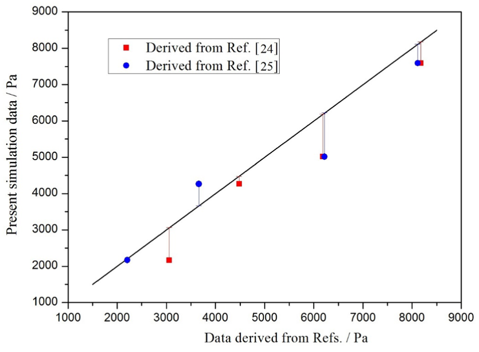
Comparison of peak-to-peak values for different speed cases.

Figure 8.

Relationship between peak-to-peak values and train speed.

Results and discussion

Flow fields

Pressure distribution

The flow field generated by two trains passing by each other in a tunnel is very complex, and it is changing constantly with running position of the train through the tunnel. In this section, the variations in the pressure distribution for two trains passing by each other in a tunnel are observed visually and discussed by selecting three typical intervals, that is, the entrance of the train into the tunnel, two trains passing by each other at the same speeds, and two trains passing by each other at different speeds.

Figure 9 shows the mean pressure around the train during the entire entrance process of the train into the tunnel. The pressure around the train in the tunnel substantially increases when the head train runs into the tunnel. Especially for the forefront of the train, the pressure dramatically changes at the entrance of the train, due to the extrusion of air by the tunnel wall. As the middle car enters into the tunnel, the pressure at the tip of the nose of the head car is approximately spherically distributed, and the maximum pressure occurs over there. The pressure distribution of flow field for the region far away from the tip of the nose varies non-uniformly along the longitudinal length of the tunnel. After the tail car enters into the tunnel, the pressure decreases rapidly and there is always a phenomenon of wake flow at the rear of the train.

Figure 9.

Pressure contour around the train during the entrance process of the train into the tunnel.

The typical pressure contours of train surfaces for two trains meeting in the tunnel at the same speed of 350 km/h are shown in Figure 10. Since the geometrical dimension, surrounding environment, and running speed of two trains are identical, the pressure distributions of the corresponding positions on train surfaces are exactly the same theoretically for two trains. This phenomenon is also demonstrated by the numerical simulation results in Figure 10. Before the two trains meet, the maximum pressure occurs near the tip of the nose of the head car. With the head car passing by each other, the magnitude of the pressure at the nose tip is gradually increased, while those regions around train bodies are consistently surrounded by negative pressure. Once two trains pass by and completely separate from each other, the pressure at the rear end of the train is significantly reduced, while the pressure at the tip of the nose tends to change from negative pressure to positive pressure.

Figure 10.

Pressure contour during two trains passing by each other at the same speed.

Figure 11 also gives the pressure contour of train surfaces for two trains meeting in the tunnel at different speeds (i.e. the observing train with a speed of 200 km/h and the passing train with a speed of 350 km/h). The change trends of pressure are generally similar to those under the same speed case in Figure 10. Because of different running speeds of two trains, the locations of two trains passing by each other in the tunnel are different from those under the same speed condition, resulting in obvious pressure differences on the surfaces of two trains. During the meeting of two head cars, the pressure around the nose region decreases rapidly, and the magnitude of the pressure and the area coverage of positive pressure at the nose of the passing train (with higher speed) are greater than those of the observing train (with lower speed). The pressure on train bodies gradually become negative during the process of two trains passing by each other. After two trains completely separate from each other, the pressure of train surfaces (especially at the tip of the nose) for the observing train tends to change from negative pressure to positive pressure.

Figure 11.

Pressure contour during two trains passing by each other at different speeds.

Velocity vector

When the train enters into a tunnel at a high running speed, it will drive the air in the tunnel to flow along the running direction of the train, which is called as “piston action” of the train,²⁶ and the resulting airflow is called as train piston wind. The train piston wind has great influence on the safety for tunnel operation and comfort of passengers.

Figure 12 presents the velocity vectors around the train at different characteristic time periods during the entrance into the tunnel. As the head car enters into the tunnel, the flow velocity of the airflow in the tunnel begins to increase, and a part of the air extruded by the train forward flows along the running direction of the train, while the rest of the air flows along the reverse direction. With the continual entrance of the train into the tunnel, the flow velocity of the air in the tunnel constantly increases; the direction of airflow in front of the train is the same as the running direction of the train, while the direction of the air between train surfaces and the tunnel wall is opposite to the running direction of the train. After the tail car completely enters into the tunnel, the airflow around the train tends to be steady, and the flow velocity also decreases.

Figure 12.

Velocity vectors around the train during the train entrance into the tunnel.

For comparison, the velocity vectors of two trains passing by each other in the tunnel at the same speed (of 350 km/h) and at different speeds (the observing train with a speed of 200 km/h and the passing train with a speed of 350 km/h) are plotted in Figures 13 and 14, respectively. Due to the different levels of the air extruded by the train during two trains passing by each other, the obvious differences of flow velocities are found compared to Figure 12. The flow velocities around the head and tail of trains are maximum, while the flow velocities of train’s bodies are minimum. In the process of two trains passing by each other, the flow velocity of the air between two trains is very low, since the air is extruded severely by trains. Similar to the analyses of pressure distribution for meeting at the same speed case, the velocity vectors of two trains are also identical, as shown in Figure 13. However, for the case of meeting at different speeds, the flow velocity of the observing train (lower speed train) is significantly larger than that of the passing train (higher speed train), as shown in Figure 14. This is to mean that the influence of the airflow on the lower speed train is much larger than that on the higher speed train, for two trains meeting at different speeds in a tunnel.

Figure 13.

Velocity vectors of two trains passing by each other at the same speed.

Figure 14.

Velocity vectors of two trains passing by each other at different speeds.

Typical features of air wave

Different from the case that the train runs in the open air, when the train passes through the tunnel, the airflow is blocked due to the restriction of the tunnel wall, and the motionless air in the front of the train is compressed severely, resulting in an abrupt increase in air and formation of air wave, which propagates through the tunnel at the speed of sound. During two trains passing by each other in a tunnel, the compression and expansion waves produced by two trains passing in and out both ends of the tunnel, combined with the air wave induced by the meeting of two trains, will be reflected continually and superimposed mutually in the process of propagation through the tunnel, resulting that the wave system is more complex than that for a single train entering into the tunnel.

The typical pressure wave history curve measured at monitor point A3 during two trains meeting in the tunnel at the same speed of 350 km/h is shown in Figure 15. When the head of the observing train enters into the tunnel, the generated initial compression wave spreads to monitor point A3 at the speed of sound, and there occur some fluctuations in the surrounding pressure at monitor point A3 due to the air disturbance by train head (in image ①). At the entrance of train tail into the tunnel, the generated expansion wave reaches this monitor point, and the pressure begins to decline (in image ②). On the other hand, when the compression wave, generated by the head of passing train entering into the tunnel, reaches point A3, the pressure begins to rise again (in image ③), and when the expansion wave generated by the tail of passing train reaches point A3, the pressure begins to decline again (in image ④). At the moment t = 3.09 s, two trains meet in the middle of the tunnel and begin to pass by each other. As the head of the passing train passes through point A3, the pressure around the measured point first increases, and then decreases and reaches the peak value of negative pressure (in image ⑤). Once the tail of passing train goes through point A3, the pressure first decreases and then increases (in image ⑥).

Figure 15.

Typical pressure wave history curve measured at monitor point A3 for a meeting speed of 350 km/h.

The pressure–time history curves of 15 monitor points on three train surfaces including the top surface and two side surfaces (as shown in Figure 5), for the condition of two trains passing by each other at the same speed of 350 km/h, are plotted in Figure 16(a)–(c). It can be seen from Figure 16 that the trend of pressure change at these monitor points is basically the same, except some slight differences for the pressure amplitudes. However, during the process of two trains passing by each other, the pressure wave curves at different monitor points on the same sides present an obvious traveling characteristic in the longitudinal direction, as indicated in Figure 16(a)–(c). For completeness, the pressure–time history curves of monitor points in the same cross section of the train (taking monitor points A3, B3, and C3 as an example) are compared in Figure 17, for the condition of meeting at the same speed of 350 km/h. Due to geometric asymmetry of the observing train passing through the double-track tunnel, the fluctuations of the pressure wave at point A3 are larger than those at points B3 and C3 when subjected to the initial compression wave generated by the train head, and the negative peak pressure value at point A3 is also larger than those values at points B3 and C3 during the process of meeting each other. The variations in pressure waves on three sides are basically the same before (expect for the duration of train head entering into the tunnel, as stated earlier) and after two trains’ meeting; this is because the pressure variations at monitor points are mainly affected by the back and forth reflections of compression and expansion waves when the trains enter into the tunnel, but not affected by the pressure waves induced by two trains’ meeting. Besides, it is also found that the variation in pressure at point C3 on the top surface is roughly the same as the corresponding value at point B3 in side B.

Figure 16.

The pressure-time history curves of monitor points for the condition of two trains passing by each other at a same speed of 350km/h: (a) on the meeting side; (b) on the non-meeting side; and (c) on the top surface.

Figure 17.

The pressure-time history curves of monitor points in the same cross-section of the train.

Variation regularity of pressure amplitudes

Here, the pressure coefficient, ΔC_P, was introduced to describe the variation in pressure wave amplitudes of monitor points on train surfaces under different meeting cases, which was defined by²¹

Δ C_{P} = \frac{2 Δ P}{ρ V_{r}^{2}}

(6)

where ΔP is the amplitude of pressure wave (Pa), ρ is the density of air (kg/m³), and V_r is the relative speed of two trains (m/s).

In the case of meeting at the same speed, the relationship between the pressure coefficient, ΔC_P, of monitor points and the normalized distance, L_i/L (where L_i is the longitudinal distance from monitor point i to the end of middle car and L is the total length of middle car), is shown in Figure 18. It is shown that the variations in pressure coefficient in the meeting and non-meeting sides with the location of monitor points are smaller for a given train speed, while the variation in the top side is larger for each train speed. The pressure coefficients of all monitor points under the meeting speed of 250 km/h are the smallest, followed by those under the speed of 350 km/h and those under the speed of 300 km/h, and those under the speed of 400 km/h (except the front three monitor points in the top side) are the largest. Besides, the relationship between the pressure coefficient and normalized distance for the case of meeting at different speeds is presented in Figure 19. It can be found that the variations in pressure coefficient with the location of monitor points are slight for all meeting cases except the condition of 200–350 km/h. For both meeting and non-meeting sides, the pressure coefficients of all monitor points for the case of 200–250 km/h are the smallest, followed by the case of 200–300 km/h and then the case of 200–400 km/h, and those for the case of 200–350 km/h are the largest. However, the pressure coefficients of monitor points in top side increase with the speed of the passing train.

Figure 18.

Relationship between the pressure coefficient and normalized distance in the case of meeting at the same speed: (a) the meeting side; (b) the non-meeting side; and (c) the top side.

Figure 19.

Relationship between the pressure coefficient and normalized distance in the case of meeting at different speeds: (a) the meeting side; (b) the non-meeting side; and (c) the top side.

Influence of train speed

Case of meeting at the same speed

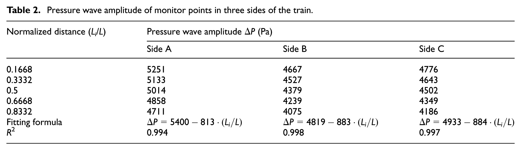
The amplitudes of pressure on train surfaces’ wave were found to be increased with the increase in meeting speed. Here, taking the case of meeting at the same speed of 350 km/h as an example, the pressure wave amplitudes of monitor points in three sides of middle car are listed in Table 2. It is seen that the pressure wave amplitude of monitor points in each side is decreased with certain extent of regularity along the longitudinal direction of the middle car. By the linear fitting, the fitting formulas between the pressure wave amplitude and normalized distance (L_i/L), and the corresponding correlation coefficients R² are presented in Table 2. The correlation coefficients are very close to 1, which indicates that the linear fitting relationship between pressure wave amplitude of monitor points and the normalized distance for each side is accurate. For more clarity, the relationships between pressure wave amplitudes and normalized distances are plotted in Figure 20, where the fitting curves are also included. To be used conveniently, a general relationship of pressure wave amplitude and normalized distance for three sides of the train is given as follows

Δ P = a - b \cdot \frac{L_{i}}{L}

(7)

where and are the two fitting constants, and the corresponding values are given in Table 2.

Table 2.

Pressure wave amplitude of monitor points in three sides of the train.

Normalized distance (L_i/L)	Pressure wave amplitude ΔP (Pa)
Normalized distance (L_i/L)	Side A	Side B	Side C
0.1668	5251	4667	4776
0.3332	5133	4527	4643
0.5	5014	4379	4502
0.6668	4858	4239	4349
0.8332	4711	4075	4186
Fitting formula	$Δ P = 5400 - 813 \cdot (L_{i} / L)$	$Δ P = 4819 - 883 \cdot (L_{i} / L)$	$Δ P = 4933 - 884 \cdot (L_{i} / L)$
R ²	0.994	0.998	0.997

Figure 20.

Relationship between pressure wave amplitudes in three sides and normalized distances for the case of meeting at the same speed.

To explore the difference in pressure wave amplitude at the same normalized distance in three sides, taking the third monitor point as an example, the corresponding pressure wave amplitudes under different meeting speeds are listed in Table 3 and presented in Figure 21, where the fitting formulas and correlation coefficients are also given. It is seen that the pressure wave amplitudes of the third point in three sides are increased with the meeting speed. All the correlation coefficients are greater than 0.9, which indicates these fittings are acceptable. The powers of the train speed in the fitting formulas are around 2.3, which are slightly greater than the value of 2 in the condition of two trains passing by each other in the open air, as a result of the effect of the tunnel entrance. The length of the tunnel in the present computational model is 500 m, due to the limitation of computational conditions; however, some studies indicate that the influence of tunnel entrance will be weakened with the increase in tunnel length, and then the power of the train speed in the fitting formula will be decreased accordingly.²⁶ This is to say, the power of the train speed may be closer to 2 for the condition of two trains passing by each other in a long tunnel in reality. As a consequence, the amplitude of pressure wave on train surfaces is approximately proportional to the square of train speed,²¹ that is

Δ P = c V^{2}

(8)

where ΔP is the pressure wave amplitude; c is a fitting constant, which is related to pressure wave and train speed; and V is the train speed. For two trains passing by each other at the same speed, the train speed V₁ = V₂ = V, and the relative speed V_r = 2V; equation (8) can also be given by

Δ P = \frac{1}{4} {cV}_{r}^{2}

(9)

Table 3.

Pressure wave amplitude of the third monitor point under different meeting speeds.

Train speed (km/h)	Pressure wave amplitude ΔP (Pa)
Train speed (km/h)	Point A3	Point B3	Point C3
200	1964	1759	1887
250	2167	1864	1941
300	4264	4119	4212
350	5014	4379	4502
400	7592	7291	7414
Fitting formula	$Δ P = 0.012 V^{2.231}$	$Δ P = 0.005 V^{2.363}$	$Δ P = 0.007 V^{2.303}$
R ²	0.954	0.916	0.914

Figure 21.

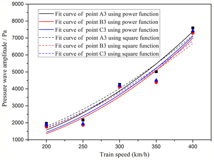
Relationship between pressure wave amplitude and train speed for the third monitor point.

Formulas (8) and (9) further illustrate that for two trains passing by each other in a tunnel at the same speed, the pressure wave amplitude is not only proportional to the square of train speed but also proportional to the square of the relative speed.

Case of meeting at different speeds

For two trains passing by each other in a tunnel at different speeds, the pressure variation on the train surface is related to the speeds of two trains. To further study the relationship between pressure wave amplitude and meeting speed of two trains, the relative speed ratio r_V is introduced by²⁷

r_{V} = \frac{V_{1}}{V_{r}}

(10)

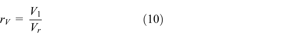
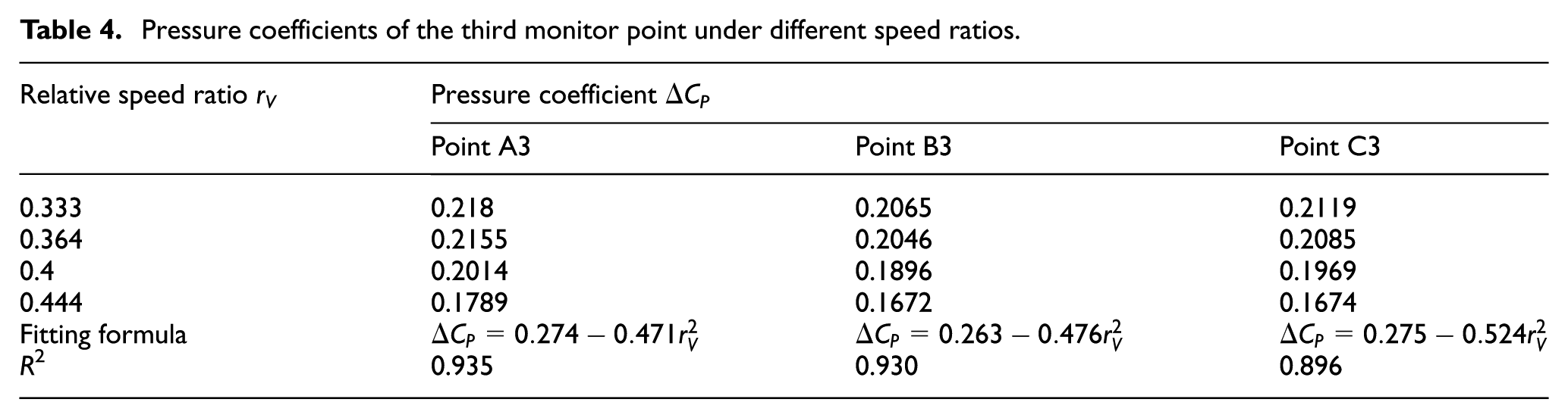
where V₁ is the speed of the observing train (lower speed) and V_r is the relative speed of two trains. The pressure coefficients of the third monitor point under different speed ratios and the corresponding fitting formulas are shown in Table 4 and Figure 22. The fitting formula with an acceptable correlation coefficient, which suggests a good correction, can be written by²⁷

Δ C_{P} = α - β r_{V}^{2}

(11)

where α and β are two dimensionless coefficients. Obviously, the pressure coefficient decreases with the increase in the relative speed ratio; for a given meeting condition, the pressure coefficient can be obtained when meeting speeds of two trains are known, and then the pressure wave amplitude can also be calculated using equation (6). Besides, for two trains passing by each other in a tunnel at different speeds, the pressure wave amplitude of higher speed train is smaller than that of lower speed train; the greater the speed difference of two trains in the meeting condition, the larger the pressure amplitude variation on train surfaces. Therefore, two trains with a large speed difference should be avoided when they pass by each other in a tunnel.

Table 4.

Pressure coefficients of the third monitor point under different speed ratios.

Relative speed ratio r_V	Pressure coefficient ΔC_P
Relative speed ratio r_V	Point A3	Point B3	Point C3
0.333	0.218	0.2065	0.2119
0.364	0.2155	0.2046	0.2085
0.4	0.2014	0.1896	0.1969
0.444	0.1789	0.1672	0.1674
Fitting formula	$Δ C_{P} = 0.274 - 0.471 r_{V}^{2}$	$Δ C_{P} = 0.263 - 0.476 r_{V}^{2}$	$Δ C_{P} = 0.275 - 0.524 r_{V}^{2}$
R ²	0.935	0.930	0.896

Figure 22.

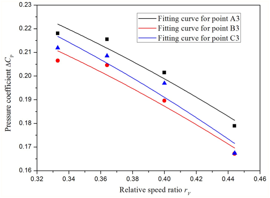
Relationship between pressure coefficient and relative speed ratio for the third point.

Conclusion

In this study, a 3D computational model of two CRH2 trains passing by each other in a tunnel was developed using FVM with moving mesh, and the characteristics of air wave and flow field around high-speed trains were investigated. Furthermore, the relationship between the pressure wave amplitude and train speed was discussed as well. The conclusions drawn from the obtained results are as follows:

The proposed computational model and approach are well-qualified to be used to investigate the characteristics of air wave generated by two high-speed trains passing by each other in a tunnel.

For the case of meeting at the same speed, the pressure distribution and velocity vectors of two trains are basically identical, while for the case of meeting at different speeds, the flow velocity of the observing train (lower speed train) is significantly larger than that of the passing train (higher speed train).

The trend of pressure change at these monitor points is basically the same, except some slight differences for the pressure amplitudes, and the pressure wave curves at different monitor points on the same sides present an obvious traveling characteristic in the longitudinal direction.

In the case of meeting at the same speed, the variations in pressure coefficient in the meeting and non-meeting sides with the location of monitor points are smaller for a given train speed, while the variation in the top side is larger for each train speed. For the case of meeting at different speeds, the variations in pressure coefficient with the location of monitor points are slight for all meeting cases except the condition of 200–350 km/h.

The pressure wave amplitudes of the third point in three sides are increased with the meeting speed, and a power function fitting relationship is obtained for the case of meeting at the same speed, while the pressure coefficient decreases with the increase in the relative speed ratio and an approximate linear fitting relationship is obtained for meeting at different speeds.

Footnotes

Acknowledgements

The authors wish to thank the National Supercomputer Center in Guangzhou, China, for access to their high-performance computing facilities.

Handling Editor: Wensu Chen

Declaration of conflicting interests

The author(s) declared no potential conflicts of interest with respect to the research, authorship, and/or publication of this article.

Funding

The author(s) disclosed receipt of the following financial support for the research, authorship, and/or publication of this article: The authors greatly appreciate the financial support by the National Natural Science Foundation of China (grant nos 51475392 and 1772275), the Fundamental Research Funds for the Central Universities (grant no. 2682015RC09), and the Research Fund of State Key Laboratory of Traction Power (grant no. 2015TPL_T02).

ORCID iD

Lin Jing

References

Tanifuji

Sakanoue

Kikko

. Modelling of aerodynamic force acting on high speed train in tunnel and a measure to improve the riding comfort utilizing restriction between cars. Vehicle Syst Dyn 2008; 46: 1065–1075.

Niu

Zhou

Liu

et al . Numerical simulation of aerodynamic performance of a couple multiple units high-speed train. Vehicle Syst Dyn 2017; 55: 681–703.

Zeng

Gretler

. Pressure wave propagation in a short tunnel caused by passing trains. Forsch Ingenieurwes 1995; 61: 304–315.

Hwang

Lee

. Unsteady aerodynamic loads on high speed trains passing by each other. KSME Int J 2000; 14: 867–878.

Zhang

et al . A multiobjective aerodynamic optimization design of a high-speed train head under crosswinds. Proc IMechE, Part F: J Rail and Rapid Transit 2017; 232: 895–912.

Sato

Sassa

. Prediction of the compression pressure wave generated by a high-speed train entering a tunnel. Int J Comput Fluid D 2005; 19: 53–59.

Miyachi

. Acoustic model of micro-pressure wave emission from a high-speed train tunnel. J Sound Vib 2017; 391: 127–152.

Raghunathan

Kim

Setoguchi

. Aerodynamics of high-speed railway train. Prog Aeros Sci 2002; 38: 469–514.

Woods

Pope

. A generalized flow prediction method for the unsteady flow generated by a train in a single-track tunnel. J Wind Eng Ind Aerod 1981; 7: 331–360.

10.

Schultz

Sockel

. Pressure transients in short tunnels In: Haerter

(ed.) Aerodynamics and ventilation of vehicle tunnels. London: Elsevier, 1991, pp.221–237.

11.

Mei

Zhou

Geng

et al . Numerical method of initial compression waves produced by a high-speed train entering a tunnel-hood based on one dimensional unsteady compressible flow model. Acta Aerodyn Sin 2006; 24: 508–512.

12.

Howe

. Pressure transients generated when high-speed trains pass in a tunnel. IMA J Appl Math 2000; 65: 315–334.

13.

Yau

RMH

Cheng

VSY

. CFD analysis of pressure fluctuation due to train passage in tunnel. BHR Gr Conf Ser Publ 2000; 43: 953–965.

14.

Chen

Hoe

et al . Field measurements of aerodynamic pressures in tunnels induced by high speed trains. J Wind Eng Ind Aerod 2012; 100: 19–29.

15.

Meng

Sun

et al . Crossing pressure wave characteristics of high-speed trains in tunnel. J Traffic Transport Eng 2015; 15: 34–43.

16.

ANSYS

Inc

. ANSYS Fluent 12.0 theory guide. Canonsburg, PA: ANSYS, Inc., 2009.

17.

Ferziger

Peric

. Computational methods for fluid dynamics. New York: Springer-Verlag, 2002.

18.

Ricco

Baron

Molteni

. Nature of pressure waves induced by a high-speed train travelling through a tunnel. J Wind Eng Ind Aerod 2007; 95: 781–808.

19.

CEN EN 14067-4:2009. Railway applications—aerodynamics. Part 4: requirements and test procedures for aerodynamics on open track.

20.

CEN EN 14067-5:2009. Railway applications—aerodynamics. Part 5: requirements and test procedures for aerodynamics in tunnels.

21.

Sun

Zhang

Guo

et al . Research on running stability of CRH3 high speed trains passing by each other. Eng Appl Comp Fluid 2014; 8: 140–157.

22.

Niu

Zhou

Liang

. Numerical simulation of the effects of obstacle deflectors on the aerodynamic performance of stationary high-speed trains at two yaw angles. Proc IMechE, Part F: J Rail and Rapid Transit 2018; 232: 913–927.

23.

Deng

Chen

et al . Unsteady simulation for a high-speed train entering a tunnel. J Zhejiang Univ: Sc A 2011; 12: 957–963.

24.

Zhang

. Study on aerodynamic performance of high-speed trains through the tunnel. MSc Thesis, Southwest Jiaotong University, Chengdu, China, 2012.

25.

Guan

Zhao

. Simulation analysis on pressure change for train crossing at the same speed through short tunnel. Subgr Eng 2011; 2: 50–52.

26.

Tian

. Train aerodynamics. Beijing, China: China Railway Publishing House, 2007.

27.

Tian

Liang

et al . Correlation between pressure wave of train passing and running speed. China Railw Sci 2006; 27: 64–67.

The characteristics of air wave induced by two high-speed trains passing by each other in a tunnel

Abstract

Keywords

Introduction

Computational model

Governing equation of fluid dynamics

Geometry modeling and computational domain

Grid generation

Boundary conditions

Computational cases

Model and approach validation

Results and discussion

Flow fields

Pressure distribution

Velocity vector

Typical features of air wave

Variation regularity of pressure amplitudes

Influence of train speed

Case of meeting at the same speed

Case of meeting at different speeds

Conclusion

Footnotes

Acknowledgements

Declaration of conflicting interests

Funding

ORCID iD

References