
Abstract
Numerical modelling is increasingly supporting the analysis and optimization of manufacturing processes in the production industry. Even if being mostly applied to multistep processes, single process steps may be so complex by nature that the needed models to describe them must include multiphysics. On the other hand, processes which inherently may seem multiphysical by nature might sometimes be modelled by considerably simpler models if the problem at hand can be somehow adequately simplified. In the present article, examples of this will be presented. The cases are chosen with the aim of showing the diversity in the field of modelling of manufacturing processes as regards process, materials, generic disciplines as well as length scales: (1) modelling of tape casting for thin ceramic layers, (2) modelling the flow of polymers in extrusion, (3) modelling the deformation process of flexible stamps for nanoimprint lithography, (4) modelling manufacturing of composite parts and (5) modelling the selective laser melting process. For all five examples, the emphasis is on modelling results as well as describing the models in brief mathematical details. Alongside with relevant references to the original work, proper comparison with experiments is given in some examples for model validation.
Keywords
Introduction
Numerical modelling is increasingly being used in the design and optimization of manufacturing processes in order to increase the quality of the produced parts and improved production yield. Today, complex manufacturing processes are often addressed with multiphysics models involving numerical heat transfer, computational fluid dynamics (CFD) and computational solid mechanics (CSM) as well as thermodynamic and kinetic models. 1 Progress in numerical modelling of material behaviour, efficient computational algorithms and advances in computer hardware and storage devices have increased the ability of complex software to be used for process design and optimization. 2
Mathematical flow simulations, also known as CFD, have matured rapidly in the last half-century. Particularly, in the manufacturing industry, use of CFD normally leads to reduced design time/cycle and improved process performance. CFD has been extensively used in metal casting and simulating the flow of molten metals in moulds.3–6 Reilly et al.7,8 have critically reviewed the role of CFD in defect entrainment in the shape casting process and summarized different numerical approaches used in different commercial packages, that is, MAGMASOFT 9 and FLOW-3D. 10 Another example of fluid flow analysis in modelling of manufacturing processes has been given by Zhang and Wu, 11 in which they investigated the effect of fluid flow in the weld pool on the numerical simulation accuracy of the thermal field in hybrid welding.
The use of CSM as another field of interest in numerical modelling of manufacturing process has also dramatically increased during the last decades. In most cases, CSM analysis is coupled with numerical heat transfer models. As an example, Schmidt et al.12,13 developed an analytical/numerical model for simulating heat generation in friction stir welding (FSW), which is based on different assumptions of the contact condition between the weld piece and the rotating tool surface. Schmidt and Hattel 14 have developed a fully coupled thermomechanical three-dimensional model for FSW using the arbitrary Lagrangian–Eulerian formulation combined with the Johnson–Cook (J-C) material law. In another study, Sonne et al. 15 studied the effect of hardening laws and thermal softening on modelling residual stresses in FSW of aluminium alloys. In their work, the Thermal Pseudo Mechanical (TPM) model is sequentially coupled with a quasi-static stress analysis incorporating a metallurgical softening model. Multiphysics modelling of welding has recently been combined with optimization methods to obtain desired properties of the weld. 16 Numerical analysis of FSW has been reviewed in the literature in general 17 and with an especial focus on modelling residual stresses. 18
The basis of most numerical simulation of high temperature processes is a proper thermal model which in many cases would be coupled with models describing kinetic and/or thermodynamic phenomena. This is very much the case for the metal casting industry which still today is a main provider of a large amount of all manufactured parts. In contrast to the traditional experimental based design of casting,19,20 numerical simulation holds great potential for increasing the productivity in the foundry industry by shortening production time. This field has been active for many years and there is still increasing effort in further developing the numerical simulation tools for variety of different casting processes.21,22
In the following, five different examples of manufacturing processes and their numerical analysis will be presented. A short introduction to each process will be given followed by some important results. The models for each of the examples will only be explained in brief; however, proper references to the original work will be given, in case more specification is needed. The selected examples are as follows:
Modelling of tape casting for thin ceramic layers;
Modelling the flow of polymers in extrusion;
Modelling the deformation process of flexible stamps for nanoimprint lithography (NIL);
Modelling manufacturing of composite parts;
Modelling the selective laser melting (SLM) process.
The two first examples deal with modelling of fluid flow, while the following two examples treat thermomechanical modelling, and finally, the last example employs a thermo-metallurgical model.
Modelling of tape casting
Tape casting is one of ceramic processes used to produce multilayer parts and substrates, like for example, capacitors, piezoelectric actuators, gas sensors.23,24 In this process, the ceramic slurry contains different ingredients, which in general influence on the rheological behaviour of the ceramic flow by increasing the viscosity magnitude and/or its non-linear dependence on shear rate (also known as non-Newtonian behaviour).25–32 However, this does not mean that assuming Newtonian (linear) explanation for the viscosity of ceramic is wrong.33,34
Fluid flow analysis in tape casting and especially in the doctor blade region and the casting reservoir (see Figure 1) is one of the most important fields of study, as it directly influences on the produced tapes. This has been the focus of researchers by developing closed-form analytical solution for the Navier–Stokes equations (combined Couette and Poiseuille flow).27–36 However, such models are limited to predicting flow front (meniscus), and hence, tape uniformity as well as thickness variation. Numerical modelling of tape casting instead will lead to optimizing the process by simulating more advanced features related to flow analysis.26,37–42
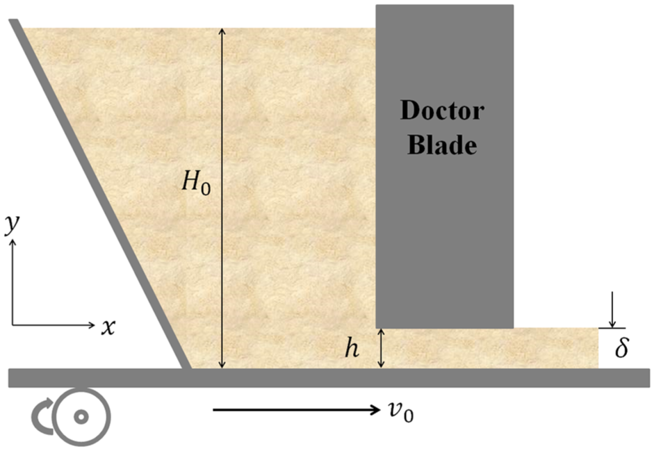
2D schematic of the tape casting process. 35
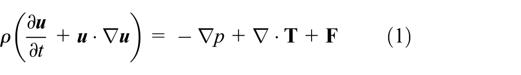
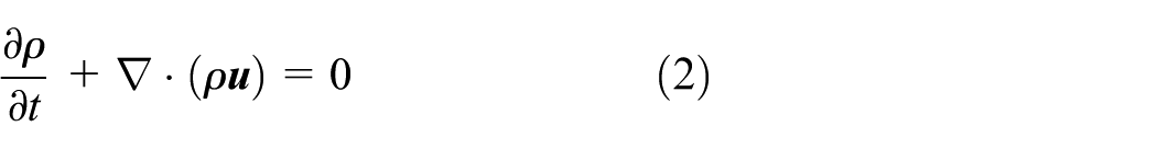
For fluid flow analysis in tape casting normally the coupled momentum and continuity equations should be solved, that is
where

where

in which

where


where
As mentioned earlier, capturing the free surface is one of the important features in the tape casting process. An example of such investigation was first reported by Loest et al.26,37 Jabbari et al.
41
developed a FVM-CFD model capable of tracking the free surface (using VOF method) combined with Ostwald de Waele–power-law flow behaviour. These developments have inherently allowed to study the tape casting process more in depth by attempting to simulate the important intrinsic phenomenon called the ‘side flow’.
40
Side flow by definition shows amount of fluid which flows in lateral direction as it leaves the doctor blade region. Jabbari and Hattel
40
reported first of a kind in literature where the side flow factor (

Modelling and experimental validation of side flow factor (
Dinesen et al.
45
have recently reported an application of tape casting for producing functionally graded ceramics (FGCs) by co-casting of two (or more) ceramic slurries. With main application in magnetic refrigeration parts, it is important to control the interface between different layers (see Figure 3(a)) to avoid mixing, and as a result increase the efficiency in a graded magnetocaloric material.
46
This interface in its ideal form has to be a 2D in-plane surface (

(a) Schematic illustration of the interface between the co-cast layers, (b) the influence of changing density and viscosity of slurry on the interface: (1)
The second stage after producing tapes is the drying process (see Figure 4(a)), in which the solvent (water or any other liquid carrier) is removed using heat and/or ventilation. 49 In this stage, there two main mechanisms which control the rate of drying namely: (1) evaporation rate of the solvent from the top surface of the tape (in contact with air) and (2) hydraulic conductivity or the rate of solvent transport to the top surface. Different kinetics are often covered in drying, that is, mass diffusion, transport in porous media, evaporation/condensation and viscous deformation, which influence the overall drying behaviour of the ceramic tapes.
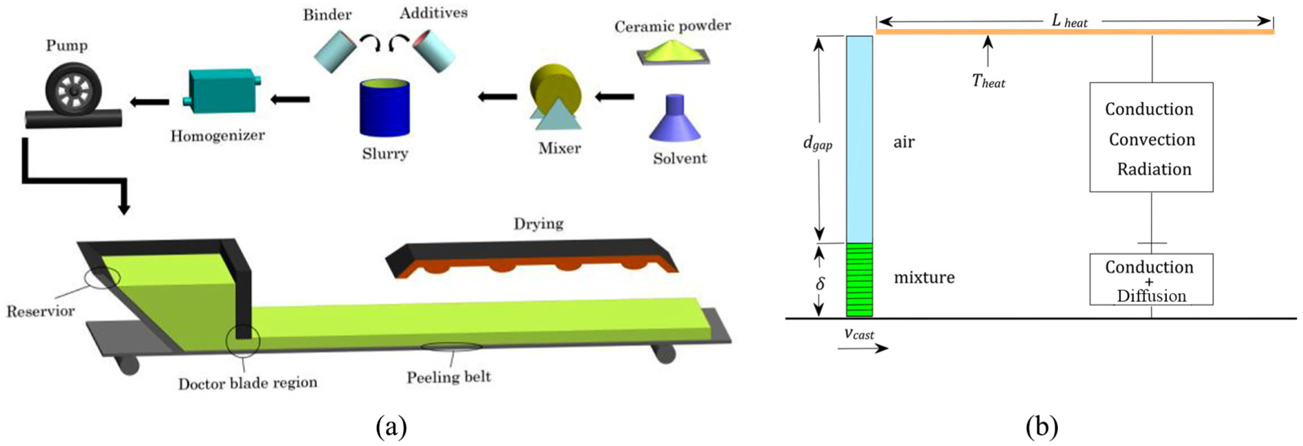
(a) Overall schematic of the tape casting process and the drying sub-process and (b) schematic illustration of the simulation domain. 50
Neglecting capillary pressure (and resultant mass transport in porous media), Jabbari and Hattel 50 numerically investigated drying of tapes by developing semi-coupled heat and mass transfer (diffusion), see Figure 4(b). Assuming water to be the solvent, a mixture of ceramic and water was considered as a representation of a tape layer. This could then serve as a relevant model system for analysing the drying process in tape casting. The results of modelling are shown in Figure 5(a) for drying tapes with initial water content of 12% and different thicknesses (δ = 400, 300, 200 μm). For the three tapes, there is initial period with no change on the water content. This is the time period that the tape temperature is rising without having evaporation, and as expected, this time period it the highest for the thickest tape.
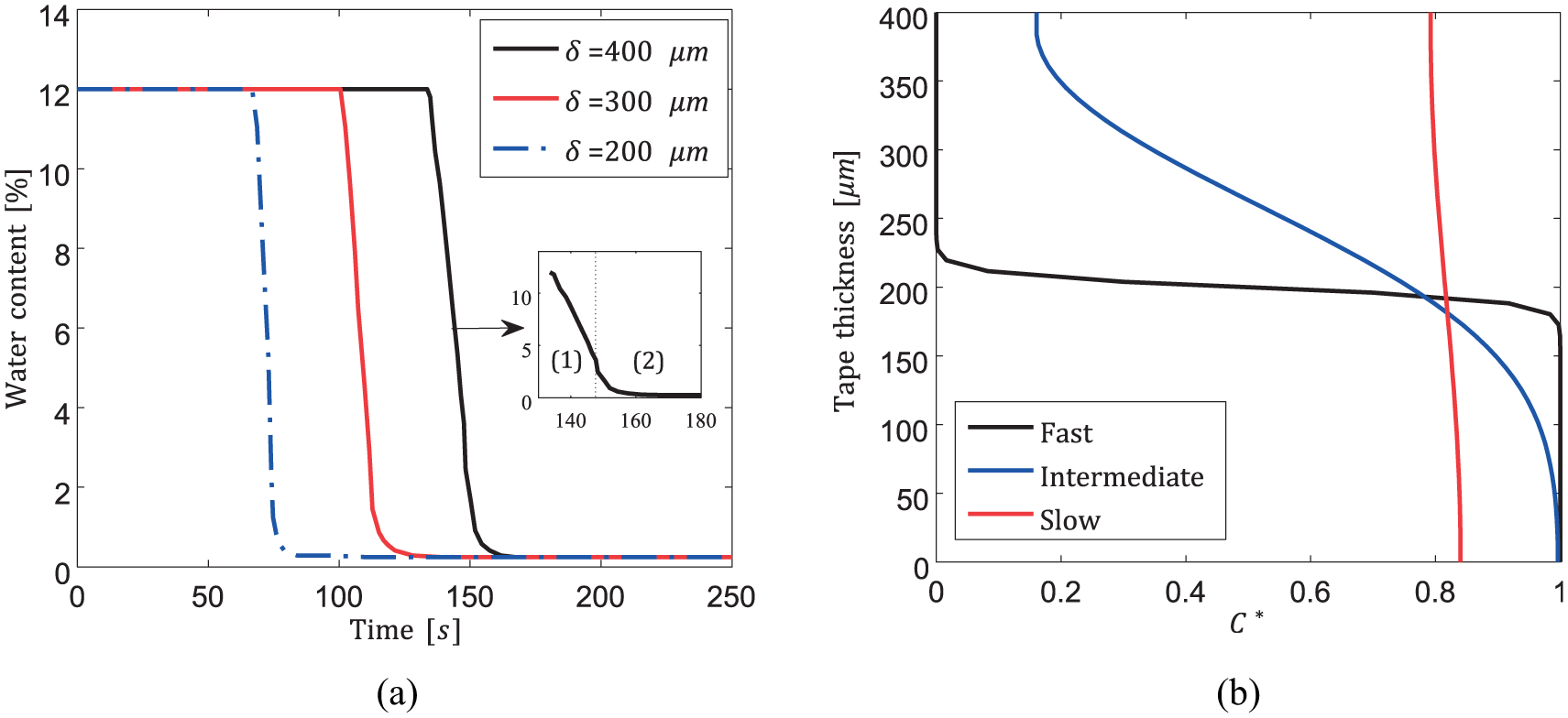
(a) Evaporation of water from a tape with different tape thicknesses (400, 300, 200 μm) and (b) the different drying modes for the tape thickness of
Three different drying modes, that is, fast, intermediate and slow, were also investigated in Jabbari et al.
50
when
Modelling the flow of polymers in extrusion
Extrusion is a common process in the plastic industry to produce long parts with a constant cross-sectional profile. The plastic material is melted and formed through a die with the desired cross-section. However, the extruded material swells at the die exit, because of the rearrangement of the flow profile after the die exit. The flow undergoes a transition from the typical parabolic profiles inside the die (constrained by the walls), towards a uniform profile outside the die (with free surfaces at equilibrium). This phenomenon is referred to as the extrudate swelling. For non-axisymmetric profiles, the swelling may also produce distortions of the extrudates. Moreover, the productivity of the polymer extrusion process is often limited by flow instabilities occurring at high extrusion speeds.
The rheological properties of the extruded materials are crucial parameters for their processability (i.e. stability and flowability). The material inside the die is subjected to large shear rate deformations, which trigger the viscoelastic behaviours of the polymers due to the stretching, reorientation and disentanglement of polymer chains. In contrast to generalized Newtonian fluids, elastic liquids build-up normal stress gradients when they are deformed in shear flows. Outside the die exit, the stretched polymer chains can recover their initial configuration, and the force balancing of the normal stress difference is responsible for an additional extrudate swelling (as compared to purely viscous fluids). Thus, taking the elastic effects into account – although not conventional yet – is desirable, in order to build accurate models of the polymer extrusion. Finally, the combination of non-Newtonian flow solvers developed within computational rheology with optimization algorithms will contribute to the development of powerful computer-aided manufacturing software, improving the extrusion processes via assisted or automated die design, according to specified optimization strategies (i.e. objective functions).57–63
The extrusion through a capillary die, sketched in Figure 6, is particularly interesting in spite of its simple geometry, because it gives an insight into the complex flow phenomena of the polymeric materials. There are different flow regimes in polymer extrusion.64,65 Figure 7 represents the typical flow curve and the regions of instabilities for the extrusion of linear polyethylene. The vertical and horizontal axes show the wall shear stress (proportional to the pressure inside the die) and the characteristic shear rate (proportional to the throughput), respectively.

Schematic view of extrusion through a capillary die.

Typical flow curve and regions of instabilities for the extrusion a linear polyethylene (reproduced from Achilleos et al. 66 with permission).
Stable extrudates with smooth surfaces are obtained at low extrusion speeds. At moderate shear rates, the sharkskin instability appears at the surface of the extrudate. The sharkskin defect produces irregular surfaces of the extrudate with superficial cracks. There is a consensus that the sharkskin defects occur at the die exit, where the material near the wall is pulled out by large tensile stress.65,67–69 The two mechanisms currently admitted to explain the sharkskin phenomenon involve either local fractures of the polymer surface outside of the die, or a local transition between stretching and disentanglement of absorbed polymer chains inside the die.65,68,69 In both cases, stick and partial slip plays important roles in the sharkskin mechanisms.64,65
At larger shear rates, the extrusion experiences a stick–slip instability (or spurt phenomenon), characterized by an alternation of smooth and rough surfaces of the extrudate, and oscillations of the pressure inside the die. The numerical analyses presented in Georgiou and collegues66,70–73 have shown that the self-sustained pressure oscillations of stick–slip instability require a non-monotonic slip law (which is consistent with both experimental data74,75 and theoretical molecular models76–78), and either the compressibility or viscoelasticity of the polymer melt in the reservoir. Thus, the slip behaviour of the molten polymer on the surface of the die is a crucial phenomenon in both the sharkskin and the stick–slip instabilities. The recent review of Hatzikiriakos 79 draws a complex picture of the wall slippage of molten polymers, with two distinct slip mechanisms: flow-induced chain desorption from the wall (weak slip), and chain disentanglement of the bulk from a monolayer of absorbed chains (strong slip). Moreover, the slip mechanisms of molten polymers are time dependent, because of the thermal degradation of absorbed polymer chains. Consequently, the inclusion of realistic slip laws in the macroscale models and the prediction of the onsets and shapes of the sharkskin and stick–slip instabilities with dynamical flow simulations are still challenging tasks. Nevertheless, the sharkskin and stick–slip instabilities can be eliminated or minimized by enhancing the slippage of the polymer, by means of chemical additives (processing aids) in the polymer formulation and/or coating on the surfaces of the die,65,80 which results in a decrease of the wall shear stress.
At larger throughput, the flow of molten polymers is subjected to the gross melt-fracture instability, which is characterized by distortions of the extruded volume. At the onset of the gross melt-fracture, the extrudate develops regular undulated or helical shapes. The distortion of the extrudate gradually looses its periodicity and eventually evolves into a chaotic regime, when the throughput is further increased. Unlike the sharkskin and stick–slip phenomena, the gross melt-fracture originates from the bulk of the molten material and is due to the viscoelasticity of the polymers.81,82 Observations by particle image velocimetry have shown that there are correlations between the periodic or chaotic extrudate distortions and upstream flow instabilities inside the reservoir.83–85 The onset of gross melt-fracture can sometimes be delayed by modifications in the reservoir geometries,65,85 without being suppressed, however. Some experimental and theoretical studies86,87 also show that the gross melt-fracture can be due to a non-linear subcritical instability of the viscoelastic Poiseuille flows, independent of the flow in the reservoir. Indeed, the elastic flow instabilities are intrinsic phenomena of the viscoelastic flows at low Reynolds numbers, which manifest themselves in various geometries.88–90
In viscoelastic flows, the relative effect of the elasticity versus the viscous forces is characterized by the Weissenberg number: a non-dimensional quantity relating the relaxation time

where
The constitutive behaviour of viscoelastic materials does not only depend on the instantaneous deformation rate

where the first term on the right-hand side corresponds to the instantaneous (purely viscous) stress response, and

where
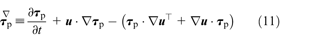
is the upper-convected time derivative, which takes into account the advection and rotation of the material in a fixed vector base. This model gives
The viscoelastic constitutive model for the extra-stress tensor is coupled with the continuity equation and the momentum conservation. These governing equations are solved with a numerical method that discretizes the geometry, for instance with finite volumes or finite elements. The Lagrangian representation of the flow (with a mesh mapped onto the deformed geometry) has demonstrated its ability to predict the steady state of stable extrusions, see for instance.91–95 However, the Eulerian representation (with a fixed mesh) seems to be best suited for time-dependent simulations with free surface flows. 96 Eulerian models have been used to simulate extrudate swelling in the stable flow regime, where the free surface outside the die was represented via an explicit surface-tracking technique, see for instance.97–99 Recent results of Tomé et al. 99 show that Tanner’s theory,100,101 which provides approximate analytical solutions of the extrudate swelling from capillary dies, did not predict the correct relation of the swelling ratio with the Weissenberg number. At large extrusion rates, the numerical simulations show a linear relation, while Tanner’s theory predicted a cubic-root dependency. Nonetheless, for Weissenberg numbers below unity, Tanner’s theory provides acceptable results which fit experimental data well. 102
Despite promising results, the numerical simulation of viscoelastic liquids is prone to an inherent numerical instability, referred to as the high Weissenberg number problem, which manifests itself by the breakdown of the simulation (i.e. blow-up of numerical values), when the Weissenberg number reaches a critical value.103,104 This has been a long-standing challenge of computational rheology, and the origins of the problem have been understood only recently. The simulations crash when the conformation tensor

a non-dimensional internal variable representing the strain of the polymer chains, which should be symmetric positive definite by definition, 105 looses its positive definiteness.105–107 Moreover, the loss of positive definiteness happens because of numerical errors dues to under-resolution of the spatial stress profiles,108,109 which may have steep gradient variations and/or be exponential, near the boundary layers and geometrical singularities. 110 A seminal reformulation of the differential constitutive model (3) has been proposed by Fattal and Kupferman.107,108 The problem is removed by a change of variable using the matrix-logarithm of the conformation tensor

In terms of
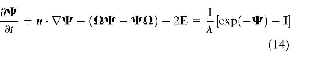
where
To the knowledge of the authors, the recent work of Kwon 111 is the only attempt of direct numerical simulations of the gross melt-fracture instability that have been reported in the literature. Kwon simulated the flow of an elastic liquid through a two-dimensional extrusion die, using the log-conformation representation with the Leonov constitutive model. 112 The geometry of the simulation included two rectilinear sections with an abrupt contraction, representing the die and the extruder reservoir. Kwon’s model neglects the inertia and the slip of the polymer melt on the die’s wall (i.e. no-slip boundary condition). The free surface of the extrudate was tracked with the Level-Set method. 113 The results presented different types of unstable extrusions, where some are qualitatively similar to the gross melt-fracture defect. The simulations showed that these extrusion instabilities originate from flow instabilities emanating from various locations within the die and reservoir, and which are only attributable to elastic effects.
A similar modelling approach has been employed by Comminal,
114
to simulate two-dimensional viscoelastic flows at the exit of a slit die. Comminal et al.
115
applied the same hypothesis as Kwon of an inertialess flow and no-slip at the walls, but used the log-conformation representation with the Oldroyd-B model and a viscosity ratio

In two dimensions, the in-plane velocity components are solely defined by the out-of-plane component

and

The streamfunction formulation removes the pressure unknown and automatically fulfils the mass conservation, by construction, in virtue of the following vector calculus identities


The pressureless formulation removes potential flaws due to the coupling of the pressure with the velocity and the extra-stress. Numerical investigations in the lid-driven cavity have shown an enhancement of the accuracy and robustness of the viscoelastic simulations. 118
In contrast to Kwon, Comminal et al.
118
modelled a slit die without reservoir (no contraction geometry). Moreover, the symmetric boundary condition was applied at the mid-plane of the die, to limit the computational costs. Hence, the simulations of unstable extrusions are constrained to solutions with a symmetric mode. The free surface of the extrudate was tracked with a recently developed volume-of-fluid advection scheme.
120
The results present stable extrudates, for low throughputs only. At the moderate Weissenberg number
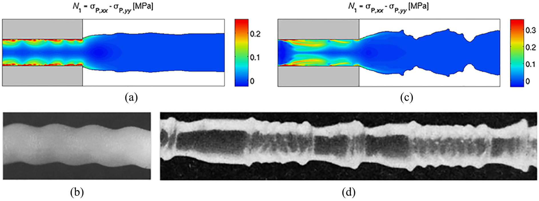
Simulated free surfaces of the extrudate and first normal stress differences inside the die, (a) for
In conclusion, it has been shown that direct numerical simulations of the gross melt-fracture phenomenon are achievable, provided that the high Weissenberg number problem is removed, for instance with the log-conformation representation. However, further work is necessary to refine the models. To date, the simulations do not include all the complex phenomena present in polymer extrusion that are attributable to non-linear slip laws, inertia and three-dimensional effects. Nevertheless, the numerical simulations remain powerful tools to discover the underlying mechanism of the gross melt-fracture and its possible link with elastic instabilities.
Modelling the deformation process of flexible stamps for NIL
Functional nanostructures on double curved surfaces have attracted increasing attention in industry. Examples of functional nanostructures are well known from nature, where organisms and plants possess optical, adhesive and self-cleaning capabilities. 123 The scientific literature is rich in examples of advanced materials emulating the well-known super-hydrophobic effect of the lotus leaf 124 and adhesive surfaces of the gecko’s feet. 125 Structural colours and iridescence are most often observed in invertebrates such as butterflies (see Figure 9) and beetles, but also in the feathers of birds.128,129 Since the early observations of functional nanostructures in nature, engineers have tried to replicate these nanostructures in order to functionalize surfaces.130–132 Recently, Christiansen et al. 127 developed a surface consisting of 1D gratings with varying wave length and orientation, resulting in a glitter colour effect, where the colour appearance is angle dependent, see Figure 9(a). The nanostructures are in first place created in a clean room, where technologies from the semiconductor industry, such as electron beam lithography (EBL) and standard ultraviolet (UV)) lithography, are applied in order to transfer the nanostructures to a silicon wafer. From there, the nanostructures are transferred to the surface of the material where the functionality is wanted via a technology called NIL a technology invented in 1995. 133

In the study conducted by Sonne et al., 134 the objective was to upgrade existing injection moulding production technology for manufacture of plastic components by enhancing the lateral resolution on free-form surfaces down to micrometre and nanometre length scales. This will be achieved through the development of a complete NIL solution for structuring the free-form surface of injection moulding tools and tool inserts. This will enable a cost-effective and flexible nanoscale manufacturing process that can easily be integrated with conventional mass production lines. The proposed technology enables functionality of plastic surfaces by topography instead of chemistry with some of the applications as describe above (e.g. colour or hydrophobic effects). A manufacturing process resembling some of the same methods as presented here, though with a nickel foil used for transferring the nanostructures, has been shown in the literature.134–136 Furthermore, other manufacturing processes associated with additive manufacturing (AM) such as direct laser writing (DLW) allow for creating sub-100 nm structures with similar functionalities as mentioned above. 137 However, the method presented in this work allows for resolutions as achieved in the semiconductor industry and the wafer-based platform makes the process competitive to the AM methods in a mass production environment. The anticipated pattern transfer method from a silicon wafer to final injection moulded plastic product is visualized in Figure 10 (this technology has been tested at pilot scale and implemented industrially 138 ). (1) A planar microstructured and nanostructured master is prepared by existing microfabrication and nanofabrication techniques such as EBL and photolithography. (2) A flexible stamp is designed, replicated from the planar master. (3) The injection moulding tool insert is coated with a polymer resist for NIL. (4) Stamping equipment is employed to imprint the flexible stamp (by a blow-moulding like process) into the double curved (free-form) injection moulding tool insert by use of compressed air. The flexible stamp is imprinted into the resist on the insert. (5) The injection moulding tool insert surface is patterned by means of electroplating or etching, using the imprinted polymer resist as a masking layer. (6) The nanostructured injection moulding tool insert is used in a conventional injection moulding process.

A flexible nanoimprint solution for nanostructuring an injection moulding tool insert. 130
For NIL on injection moulding tool inserts (and on double curved surfaces in general), the deformation and stretch of the flexible stamp can be up to 50% and in the millimetre range. 139 This is problematic since even very small changes in the nanostructures geometry will change the wanted overall functionality. 140 The deformations are therefore important to take into account, when the planar silicon masters are designed. Here simulation tool such as the finite element method (FEM) is an appropriate way of predicting those deformations. Numerical models for simulating the NIL process in general have been shown in the literature,141–144 with the main purpose of solving for the flow of resist and the local stamp bending, with the classical squeeze flow model (the Stefan equation 145 ) as benchmark

where
The Stefan equation is however not directly suitable for the NIL on curved surfaces due to a number of different aspects that complicates the overall physics: (1) Because of the large deformations and hence strains in the flexible stamp, non-linear geometry has to be taken into account in order to get accurate results from the numerical simulations. 146 (2) The material behaviour is non-linear and is for the polymer material described by a viscoelastic–viscoplastic constitutive behaviour.147,148 (3) With respect to the contact conditions, changes in frictional behaviour on the different length scales (macroscale to nanoscale) have to be taken into account149–152 and add yet another nonlinearity to the system of equations that have to be solved. Here, multiscale modelling is an approach where the global and local conditions can be taken into account in the same model. 153
In the work done by Sonne et al. 134 a standard continuum mechanics was applied with the overall goal of solving the three static equilibrium equation

where


where
where
The model has been verified through a series of experiments, where NIL on a double curved tool insert for injection moulding (Figure 11(a)) was performed with different process parameters. The outcome of the model is first of all contour plots of the maximum principal strain field on the geometry of the deformed flexible stamp (see Figure 11(b)). This will give an indication of how much the nanostructures have been stretched during the nanoimprinting process. Furthermore, the transient pressure distribution between the mould and flexible stamp can be examined and used to optimize the process parameters in terms of imprinting temperatures and pressures and the thickness of the flexible stamp.

(a) The used flexible stamps with the glitter effect nanostructure on top of the steel tool insert after nanoimprint. (b) Numerical model of the same setup where it is possible to study the strain field within the flexible stamp in combination with the actual imprinting pressure underneath the flexible stamp. 130
For the application shown in Figure 11, good agreement between simulations and experimental results in terms of maximum principal strain was found, see Figure 12.

Comparison of measured and calculated maximum principal strains along two different paths on the deformed flexible stamp. 130
In general, both experiments and simulations have shown a mismatch between the defined and measured nanostructures as a result of stretching of the flexible stamp. This clearly indicates the necessity for numerical models in order to take this deformation into account when the nanostructures are designed in the first step of the process. The developed models have shown to predict the stretch of the nanostructures with a maximum error of 0.5% defined as the difference between measured and simulated wave lengths of the nanostructures on the surface of the deformed flexible stamp, 130 indicating their ability to capture the essential physics of this manufacturing process.
Modelling manufacturing of composites
Fibre-reinforced polymer (FRP) matrix composite materials have found widespread use in the manufacture of large energy critical structural applications such as wind turbine blades where low weight and high strength are crucial. In the wind energy industry, the use of FRP composites in large wind turbine blades has surpassed all other materials for both the load-carrying and airfoil sections of the blades. 159 Composites offer a low weight-to-stiffness ratio and user-defined high durability and strength. Application-defined properties are also more readily obtained by tailoring the composite lay-up, thicknesses and fibre/matrix combinations according to the mechanical, thermal, electrical or aesthetic requirements. During the manufacture of thermoset polymer composites in general, the reinforcement fibre material is moulded into a desired shape by impregnation and curing of the fibres with a liquid polymer resin, typically a thermosetting epoxy or polyester. Upon curing a structural unified solid combination of these materials is achieved, resembling the mould geometry. Many different variations of this basic process exist, for instance pultrusion,160,161 filament winding,162,163 resin transfer moulding (RTM),164–166 vacuum infusion (VI), 167 vacuum-assisted resin transfer moulding (VARTM), 168 to name a few. 169 In this article, focus is on two different processing methods: pultrusion and VARTM, see Figures 13(a) and (b), respectively. The combination of thick geometries, cure cycles at elevated temperatures and the highly non-linear resin phase transition characteristics and release of latent heat can make the process complex to control.170–172 Furthermore, avoiding process-induced shape distortions and residual stress build-up remains a challenge in many applications. 173

(a) Schematic view of the traditional pultrusion process and (b) schematic illustration of VARTM.
Only the main features of the needed theory for modelling of composite manufacturing will be outlined here. In order to analyse the thermal conditions during processing, the energy equation must be solved

Note here that the material flow during processing is taken into account via the advection on the left-hand side, where
Thermoset resins also exhibit volumetric shrinkage during curing, sometimes as high as 9% for polyesters. Moreover, as the resin develops from the viscous state to the solid state, large changes in the thermal and mechanical properties occur. Johnston 174 proposed a modified linear elastic model incorporating temperature dependency which also allows thermal softening.171,175,176 This model which is often denoted the model cure hardening instantaneous linear elastic (CHILE) model is used in the present work. This indicates that with an increase in degree of cure, the modulus increases monotonically. User-defined subroutines are developed in ABAQUS for the constitutive material models. The corresponding expression for the CHILE model is seen in equation (26) 177

where

where
The effective mechanical properties as well as thermal and chemical shrinkage strains of a laminate are calculated using a micromechanics approach, for example, the self consistent field micromechanics (SCFM) approach which is a well-known and documented technique in the literature. 178
During composites processing, manufacturing-induced strains are known to develop as a result of the matrix material chemical cure shrinkage in combination with thermal gradients as well as mismatch in thermal expansion properties. 179 More specifically, knowing the isotropic resin shrinkage strain, the incremental longitudinal and transverse chemically induced shrinkage can be determined for a composite material taking micromechanics into account. Thermal strain increments are calculated in a similar manner based on the temperature change and the composite effective thermal expansion coefficient. Since strains are in general small, linear strain decomposition can be used such that the process-induced strains are expressed as the sum of the thermal strains and chemical strains and finally the total strains are hereafter found from adding the mechanical strains and process-induced strains. At each time step, the properties of the rein are updated. Using the SCFM approach, the effective properties of the composite laminate are then calculated in which the fibre properties are assumed to remain constant. 180
Numerical modelling of pultrusion
Pultrusion is a cost-effective production process for manufacturing FRP composite profiles. Constant cross-sectional profiles are produced in a continuous manner. The resin material impregnated the fibre reinforcements in a resin bath system while being pulled by a pulling mechanism. Curing takes place inside the heater pultrusion die. A saw is often used to cut the profile into desired length. A schematic illustration of the process is seen in Figure 13.
Pultrusion process has been analysed using various thermo-chemical numerical models since 1980s in order to control the curing and temperature distribution during processing.181,182 Some of the thermo-chemical computational analyses can be found in previous works.183–188
Baran et al.119,189,190 have made the first thermo-chemical-mechanical model of pultrusion in which a coupled thermo-chemical-mechanical is developed using ABAQUS and used to model the pultrusion of the L-shaped profile as shown in Figures 14 and 15. In Baran et al., 191 a more comprehensive mechanical model was proposed to analyse the process in 3D by calculating the stresses and shape deformation. A glass/polyester was considered in Baran et al. 119 for the UD as well as the CFM layers, and for the die, a chrome steel was used. As shown in Figure 15, the heating regions were 275 mm long and 60 mm wide and they were placed 150 mm apart from each other. The length of the die was 1000 mm and the post-die region was 5000 mm long. The surfaces of the composite at the post-die region were exposed to convective cooling boundary condition. Similar boundaries were also defined for the die surfaces except the heater regions. The polyester resin entering the die inlet was assumed to be at uncured viscous state and the curing took place with the help of heaters. The necessary material properties were characterized in Baran et al. 177 such as curing kinetics, temperature and cure-dependent elastic modulus and viscosity.

Pultruded L-profile. 119

Pultrusion setup of L-shaped profile with dimensions indicated. 119
The generalized plane strain elements CPEG8R available in ABAQUS were used in the 2D quasi-static mechanical analysis. Figure 15 shows the 2D cross-section of the L-shaped profile. A Lagrangian framework was applied in the 2D mechanical model such that the temperature and cure distributions calculated in the 3D thermo-chemical model as well as the mechanical boundary conditions were updated at each quasi-static time step. 192 The model predicted the stress–strain development as well as the nodal displacements. 192
The predicted spring-in angle as a function of the pulling distance is depicted in Figure 16 (left). It is seen that the deformation process of the profile continues until around 6 m away from the die-exit during the cooling stage in air. The final spring-in angle as a function of different pulling speeds from 500 to 1000 mm/min is depicted in Figure 16 (right). It was found that the spring-in angle increased with pulling speed. Moreover, the final spring-in for parts produced with a pulling speed of 600 mm/min was measured and good agreement with the predicted value was found.

Left: Predicted spring-in angle of L-shaped profile as a function of the pulling distance. Right: Predicted spring-in angles for different pulling speeds (compared with experimentally found value for 600 mm/min 119 ).
In Baran, 193 the process-induced residual stress development was described for a 100 × 100 mm pultruded square profile made of glass/polyester. The temperature and degree of cure distributions were calculated for three different preheating temperatures. The nonuniform internal constraints in the part yielded in an internal shear deformation during the process. The transverse shear stress and compressive normal stress levels decreased significantly as compared with the tensile normal stresses with an increase in preheating temperature. Predicted transverse shear stress distributions are depicted in Figure 17.

Transverse shear stress distribution (
The mechanical properties of the fibre-reinforced composite materials might vary significantly due to the manufacturing-induced effects. 194 The possible causes for this variation can be the nonuniform distribution of fibre/matrix, fibre misalignment, residual stresses at micro and meso level, dry spots and voids due to poor impregnation and so on. The probabilistic and reliability analyses of the pultrusion process were studied in Baran et al.195,196 The variability in the product properties and their effects on the curing and temperature were investigated. In addition, the process conditions were optimized in several studies for the pultrusion process.197–200
Modelling process-induced strains and stresses in a thick laminate plate
The internal strain development during curing of a thick laminate plate at elevated temperatures using a long cure cycle was analysed by Nielsen et al.175,176 The objective with the study was to evaluate how accurate the aforementioned CHILE constitutive model is at predicting the internal strain development, in what is essentially a viscoelastic problem. 3D numerical model total strain predictions are compared with experimentally determined in situ strains within the laminate part, using embedded optical fibres with fibre Bragg grating (FBG) sensors. Hence, a direct comparison can be made with model predictions, capturing how thermal expansion and chemical shrinkage strains develop within the laminate throughout curing during the VI moulding process, as well as the influence of tooling.
A glass/epoxy UD laminate was manufactured using the VI techniques. The dimension of the laminate was 400 × 600 mm consisting of 52-layer UD E-glass fibre mats. A tempered glass of 10 mm thickness was employed as a mould.175,176 Prior to infusion, sensors were embedded within the dry preform; including thermocouples and optical fibres (FBGTop, FBGCenter and FBGBottom), each consisting of three FBG sensors interspaced along the optical fibre, see Figure 18(a). The optical fibres were placed transversely to the main reinforcement fibre direction in order to capture the matrix-driven process strains. The laminate was vacuum infused and cured at 40°C on a heated plate.

Schematic of (a) exploded view showing the embedded sensor placement, (b) laminate and tool plane of symmetry and (c) mechanical contact conditions assumed. 175
A sequentially coupled thermomechanical numerical analysis was subsequently conducted. Symmetry conditions were assumed why only half of the laminate plate and tool was modelled (Figure 18(b)). In the thermal step, Dirichlet boundary conditions (known temperatures) were prescribed on the laminate plate top and bottom surfaces, as determined experimentally. Moreover, the heat flux through the symmetry plane was neglected. In the mechanical step, a tied condition at the tool/part interface was prescribed, mimicking perfect bonding between the tool and laminate during the process. This condition is a simplification of real-life sliding, sticking and other cohesive interfacial contact conditions. In the model, it was assumed that the preform is perfectly impregnated through the use of a constant fibre volume fraction resembling the final state of the part after processing. 171 Demoulding is modelled after curing at ambient temperature by simply suppressing all mechanical constraints between tool and part.
Figure 19 presents the experimentally determined centre plane laminate temperature (T2), compared with model predictions of temperature and corresponding cure degree model predictions. Upon commencement of the curing reaction, an increase in temperature is seen as a result of heat generation during the release of latent heat upon matrix cross-linking. After the temperature peak, a steady-state temperature is upheld corresponding to approximately 40°C, after which the laminate cools to ambient temperature. It is seen that a substantial amount of curing develops prior to when the exothermic peak temperature is reached. This relates to the autocatalytic equation for the cure rate being self-catalysed by increases in temperature. 171
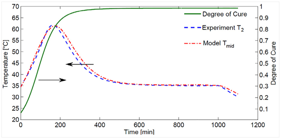
Experimental laminate mid-plane temperature and model prediction. Also shown is the corresponding modelled cure degree development. 171
Figure 20 shows the comparison of the predicted transverse strains with the measured ones at the centre of the laminate (mid-plane). The total strains are seen to relate somewhat to the thermal profile presented in Figure 19, deferring mainly due to the influence of chemical cure shrinkage. Good agreement between the model predictions and the experimentally measured strains is observed, with the best agreement early in the process. As the resin cures, the strain development goes from being driven by the tool expansion due to the tied contact, to being driven by the induced thermal and chemical shrinkage laminate strains.

Process-induced total transverse strain comparison between model predictions and experimental data. Also seen is the predicted cure degree development at the laminate plate centre. 171
The influence of the tool (tempered glass plate) is visible upon cooling, that is, at time of 1050–1300 min. It is seen that a smaller gradient is present on the predicted total strain curves as compared to the experimentally determined strains. This may be due to the lower coefficient of thermal expansion (CTE) of the tempered glass plate (
Thermo-metallurgical modelling of SLM
Modelling of thermal conditions during manufacturing processes and resultant metallurgical features is a well-established field of research.201–208 In the case of SLM, however, the application of these techniques of microstructure predictions is still limited. Nonetheless, the plethora of experimental studies in the literature focusing on characterizing and empirically predicting the microstructure during SLM of materials209–212 clearly indicates the scope and need of thermo-metallurgical modelling studies.213,214 In this section, a brief overview of the work carried out on thermo-metallurgical modelling of SLM is presented. Subsequent to a brief outlining of the theory associated with the thermo-metallurgical model, the evolution of centre-line microstructure during single melt track formation is simulated and discussed.
SLM 215 process was developed in Fraunhofer Institute for Laser Technology in Aachen, Germany and it has since been a prominent centre for research in SLM. Together with selective laser sintering and electron beam melting, it is among the most prevalent form of metal AM. Potential target areas providing significant scope for SLM include aerospace applications, automobiles and medical implants. Due to the clear advantages of such an AM process, SLM has been the subject of intense research in the last decade. SLM and similar metal AM processes have been reviewed in previous works216–224 from experimental and modelling perspective, including current practices and future challenges regarding raw materials, processing and post-processing.
The SLM process begins after a sliced 3D CAD model is received by the machine. The sliced model contains information about the zones to be melted in different layers. A powder scrapper moves some powdered material from the feed container onto the build platform, distributing it more or less uniformly. Then the laser beam source is turned on. Typically, a Nd:YAG or CO2 laser having a Gaussian energy distribution is used as a power source for selectively melting certain zones in a layer of powdered material, which eventually give rise to a 3D structure (Figure 21). The generated beam is deflected by scanner mirrors which control the movement of the laser beam over the powder surface. The beam is focused by the help of a lens that can alter the focusing distance and the divergence of the beam. Depending on the input from the sliced 3D model, the laser beam melts out a shape in the powder layer. Upon completion of the laser treatment, the build platform moves down by a fixed amount and another layer of powder is scrapped onto it. The process is repeated until the complete 3D object is created. The entire process is carried out in an inert atmosphere of argon or N2 with continuous gas flow through the chamber.

Schematic representation of heat transfer during selective laser melting. 225
In SLM process, the melt pool size (typically in the range of 100–500 μm) is small enough compared to the size of the component being manufactured that conduction becomes the primary mode of heat transfer in the entire domain. In such a case, the spatial and temporal distribution of temperature is governed by the heat conduction equation, which can be expressed as

where

where
One of the most common material property for which an equivalent value is required when using a conductive heat transfer formulation is the emissivity of the powder bed. The current work is based on the predictive models proposed by Sih and Barlow231–233 wherein a combination of the emissivity of the particles and the emissivity of the cavities in the powder bed is used

where

Similarly, effective thermal conductivity values also need to be found for the powder bed as well as for molten/vaporized materials. A modified version of the Zehner–Schlünder–Damköhler model found in the literature, which describes a randomly packed powder bed formed of mono-sized spherical powder particles, can be used to calculate the equivalent thermal conductivity as

where

where

Similarly, for properties related to laser–material interaction such as albedo, scattering coefficient, extinction coefficient, equivalent values need to be calculated. While the involved physics can typically only be modelled via differential and integral equations, simple empirical models drawing upon experimental results do exist in the literature. For instance, the extinction coefficient (


Apart from calculation of equivalent material properties, the heat conduction equation also needs to be provided with appropriate heat source term
where

where
The internal state variable approach 238 is well suited to the development of models for non-isothermal microstructural evolution. In general, a microstructure may be defined by different state variables such as grain size, volume fraction of grains, fraction of solid in solidification. For the current case of solidification, two internal state variables can be used to describe the microstructure evolution – namely temperature and fraction of solid. The usage of these two state variables for modelling solidification microstructure is described below.
The interaction of the two state variables (temperature and fraction of solid) determines the type of microstructure formed during solidification. All grains produced during solidification are assumed to be equiaxed in nature, with columnar grains considered to be similar to elongated equiaxed grain.
The equiaxed solidification begins with nucleation in the regions of melt pool just below liquidus temperature and along the boundary of the melt pool. Although nucleation is a randomized phenomenon, statistical models exist for characterizing the overall nucleation in a melt pool. The Oldfield model 239 is most popular wherein the nucleation distribution is described by a Gaussian distribution. The grain density at a particular undercooling is given by

where
Nucleation can occur in a homogeneous or heterogeneous manner; however, the latter is much more common due to less energy requirements. The heterogeneous nucleation in the above model is assumed to be instantaneous and dependent on the characteristic undercooling. Once nucleated, the grains start to grow outwards. This results in the fraction of solid in the local melt pool area increasing, and there is corresponding release of latent heat of fusion which might increase the local temperature(this phenomenon is called recalescence). The grain nucleation is also random with respect to the orientation of the grain. Thus, to distinguish between different grains, a characteristic misorientation angle is attributed to each grain with respect to one of the principal direction (Figure 22).

Schematic diagram illustrating the growth algorithm used in the cellular automata model for a dendritic grain whose
Dendritic grain growth is assumed to be primarily driven by thermal undercooling and curvature undercooling. The kinetic undercooling and solute undercooling are ignored for the present work, although they are known to be important especially when in case of liquids with high Peclet number. The adopted grain growth model is similar to that described by Gandin and Rappaz. 240
The model focuses on the envelope outlining the dendrite tip positions. In grains with four dendritic arms as in (corresponding to
The growth of the grain is associated with the length of the dendrite tip which in turn depends upon the growth kinetics. For a grain nucleated at time

where

with the contribution of thermal undercooling

where

The radius of curvature of the dendrite tip is a function of the thermal Peclet number and is given by


where
The modelling of microstructure for SLM is performed using a sequentially coupled 3D FVADI thermal model 228 and a 2D Cellular Automata microstructure model. The cellular automata model and implementation of grain nucleation and grain growth models are explained below.
A cellular automata is a discrete model consisting of a regular grid of cells, each in one of a finite number of states. For each cell, a set of cells called its neighbourhood is defined relative to the specified cell. The two most common descriptions of neighbourhood are Moore’s neighbourhood (all eight cells surrounding a square cell) and the von Neumann neighbourhood (the top, bottom, left and right adjacent cells). An initial state is selected by assigning a state for each cell. A new generation is then created according to some fixed rule that determines the new state of each cell in terms of the current state of the cell and the states of the cells in its neighbourhood. Typically, the rule for updating the state of cells is the same for each cell and does not change over time.
The grain nucleation phenomenon is modelled in the cellular automata model in a probabilistic manner. Each cell of the cellular automata model is prescribed a random probability of nucleation which indirectly corresponds to a random distribution of critical undercooling. For nucleation to take place in a cell

where
In the current implementation, the mathematical function (rule) governing the cellular automata is based on the growth of grain, more specifically the growth of the dendritic arms of the crystal. The rules can be set as follows:
Rule 1: The dendritic arm of a cell can start to grow only if the cell has been nucleated or captured by an adjacent grain.
Rule 2: The dendritic arm of a cell in a direction can grow only if the adjacent cell in that direction is below the liquidus temperature and has not already been nucleated or captured by another grain.
Rule 3: Once captured by a dendritic arm from an adjacent cell, a cell gets the same state (misorientation) as the cell capturing it and is assumed to possess dendritic arms of same length as the capturing cell in the orthogonal direction to that of the capturing dendritic arm.
For the purpose of capturing an adjacent cell, the grain envelope must reach the centre of the adjacent cell. For the grain shown in Figure 22, this corresponds to the situation when

where


As per the cellular automata rules, the growth of cell
In the particular implementation, only equiaxed grains are considered, and therefore, the growth of dendrite arms in the four directions for a cell is the same and only based on the local undercooling. In case of columnar grains, however, the growth might be preferred along certain direction over the others.
The 3D FVADI and 2D CA models are coupled sequentially with the 3D FVADI model providing the temperature field. To take into account the release of latent heat, equivalent specific heat capacity values are used during calculations. The temperature field calculated from the 3D FVADI model thereby governs the undercooling occurring at each cell in the 2D CA model. As the thermal calculations are performed at a larger spatial and temporal discretization, the values are interpolated in the corresponding domains to match the requirements of the cellular automata. As a thumb rule, the spatial discretization of the CA model is near the order of the radius of dendritic tip, and the time resolution is such that the dendrite tip can only grow till the next adjacent cell at a maximum chosen undercooling.
The centre-line microstructure of a single melt track is modelled using the 3D FVADI–2D CA model. The parameters used for the thermal model are shown in Table 1 and the parameters for the microstructural model in Table 2.
Parameters for thermal model of single melt track formation. 237

Parameters for microstructural model of single melt track formation. 237

The thermal model was used on a domain of
Figure 23 shows the temperature field obtained from the thermal model at four time instances during the simulation of single melt track formation. The black rectangular borders shown on the figures correspond to the area selected for microstructure modelling using cellular automata. Figure 24 shows the solidification microstructure at the corresponding times. The grains are initially nucleated at the solid–liquid interface as can be seen in Figure 24. Although simulated on a structured grid, the grains maintained their misorientation during growth which resembles real grain growth mechanism. Most of the grains are seen to be oriented at a large angle to the direction of laser movement (also commonly observed phenomena), which is a result of the grains growing normal to the solidification isotherm.

Centre-line temperatures at four time points during single track formation with SLM. 237

Evolution of centre-line microstructure at four time points during single track formation with SLM. 237
For simulation of microstructures which can be validated against experimentally generated single track, the model would require several parameters which need to be determined experimentally such as the maximum nucleation density, the mean undercooling, the radius of unit thermal undercooling. In addition, the model would need to be extended to include solute diffusion and kinetic undercooling.
For comparison with single track which is allowed to cool under processing conditions, the model would also require to include the recrystallization occurring at

Monte Carlo simulation based on 2D Potts model for
The thermo-metallurgical model was able to predict the representative microstructure observed during single melt track formation on a loose powder bed using SLM. The small size of melt pool and the high cooling gradient, especially in case of low Peclet number materials, allows neglecting certain otherwise important terms from the grain growth models. However, it would be necessary to include them in case of high Peclet number material such as 316L steel. In addition, the evolution of solidification microstructure from SLM into the final
Conclusion
Modelling and simulation of manufacturing processes is a truly interdisciplinary field spanning mathematics, computer science, heat transfer, fluid and solid mechanics as well as materials science and manufacturing engineering. Models allow us to create mathematical representations of the system under investigation and simulate its properties and behaviour over time and under different conditions. This is an extremely powerful approach in planning and understanding experiments and producing predictions in designing manufacturing systems and increasing their efficiency. Modelling and simulation techniques are used in all realms of science and engineering and find endless industrial applications.
The present paper presents five cases of modelling different aspects of modern manufacturing processes ranging from fluid flow analysis (tape casting of ceramics and extrusion of polymers) over thermomechanical analysis (NIL of features on the surface of injection moulding dies and composite manufacturing) to thermo-metallurgical analysis in SLM. For some of these areas, selected results from numerical modelling have been compared with corresponding experimental findings and good agreement has been found. It is evident that models and simulations like the ones presented here will further increase their use in the future as an important part of analysing the effect of selected materials and process parameters on the subsequent performance of manufactured parts.
Footnotes
Handling Editor: Filippo Berto
Declaration of conflicting interests
The author(s) declared no potential conflicts of interest with respect to the research, authorship and/or publication of this article.
Funding
The author(s) received no financial support for the research, authorship and/or publication of this article.