Sage Journals: Discover world-class research

Abstract

In order to improve the stability and the lifespan of rotating components in a canned motor of a centrifugal pump, a local hydraulic loss analysis has been performed based on detailed flow field analysis by Reynolds-averaged Navier–Stokes–based re-normalization group k-ε turbulence model simulation. An energy balance equation was applied to analyze the local hydraulic loss distribution. The stator flow channel in the motor was modeled as a porous medium, by utilizing the Ergun equation. Due to the complex structure and the velocity gradient in the complicated flow field, a strong circulation flow exists in the thrust bearing outer ring. Moreover, circumferentially asymmetric Taylor vortices in the vicinity of the hydrodynamic bearing and unsymmetrical Taylor vortices in the transitional region after the thrust bearing were predicted. Dean vortices in the distributary pipes are also captured. These complex vortices are accompanied with high dissipations. A strong increase in hydraulic losses are observed in the corresponding canned motor parts (x/x_max = (0.03, 0.23), (0.87, 1)). Moreover, a strong increase in the radial force and the axial force are predicted in the relative parts of canned motor (x/x_max = (0.84, 0.97), x/x_max = (0.24, 0.17), (0.84, 0.97), respectively).

Keywords

Canned motor shaft forces hydraulic losses porous media flow typical vortex

Introduction

Canned motor is characterized by its high power density, tight structure, low noise, high efficiency, and zero leakage.¹ With the increasing demands for compact structures and low costs, as well as the development in new topologies and materials, heat dissipation in the motor has attracted a wide research attention. As the main structure in the canned motor, shaft has a great influence on the stable and reliable operation of the rotor system, in terms of its performance under rotations. For example, instability and asymmetry of the flow field in the shaft system will influence the shaft forces of the motor significantly, causing the axial float of rotating components, shell wearing, and the increase in the bearing load, thus shortening the service life of the motor.

Generally, shaft forces in similar canned motors are calculated either from empirical formulae of material mechanics or integrated directly from the pressure distribution on the shaft surfaces by computational fluid dynamics (CFD) simulation. Young² analyzed the integrity and lifespan of a shaft sleeve based on fracture mechanics, subject to surface temperature fluctuation. Zhang et al.³ investigated a propeller shaft system using Hamilton’s principle in conjunction with the finite element method. Analytical and numerical results show that friction-induced vibration of the shaft system is due to the combined action of nonlinear friction and coupled dynamics of the system. Liu et al.⁴ studied the temperature field in the bearing of a hot water circulation pump by a finite element model. Steady temperature field in the shafting structure shows that the motor temperature close to pump stent is slightly higher than away from stent. Based on the finite element method, Wang et al.⁵ carried out a static flow analysis of the shaft-seal nuclear coolant pump, to verify the shaft strength and stiffness. This study provided a reference for the research and design of large vertical rotating body. Existing analyses on shaft forces of a canned motor are based on presetting of total forces. Unfortunately, methods in literature have not considered the flow pattern in motor stator channel and its impact on shaft forces. Furthermore, they ignored complicated gap flows and intensely circular turbulence that can affect shaft forces significantly. Specific impacts of the vortical flows on shaft forces in canned motors have not been discussed from the perspective of hydromechanics.

Based on previous hydraulic and mechanical optimization of a centrifugal boiler circulating pump,⁶ in order to accurately capture different flow regimes (laminar flow and intensely circular turbulence) in a canned motor, a high-precision CFD approach was presented. Impacts of circulation flow and pressure distribution in a canned motor on hydraulic losses and shaft forces were investigated. This article also systematically analyzed the pressure distribution, flow patterns, and flow characteristics with different internal structures of the canned motor. Locations and causes of different vortices, energy conversion and dissipation, and force distribution in the motor were also analyzed.

The remaining parts of this article are organized as follows. In section “Methodology,” the configuration of the model motor, and the numerical methods adopted in this study are described. Reynolds-averaged Navier–Stokes (RANS) equations and re-normalization group (RNG) k-ε turbulence model, a governing equation of the porous medium and relative resistance coefficients of porous medium are applied in the study. In section “Initial boundary conditions and grid partitioning,” the initial and boundary conditions for flow simulation are given. Structural grid partition strategy and the process are described briefly. In section “Results and analysis,” numerical calculations of the circulation flow in the canned motor with porous medium are presented, and the corresponding results are analyzed in detail. The formation of the (Taylor and Dean) vortices in the relative domains of the canned motor is discussed. Hydraulic losses of the canned motor are analyzed. The impacts of the above flow patterns on shaft forces are analyzed. Finally, in section “Conclusion,” the summary and conclusions of this study are provided.

Methodology

Computational domain

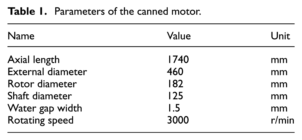
To describe the configurations of the complicated motor flow field accurately, the computational domain is divided into eight parts: (1) inlet channel, (2) thrust bearing, (3) transition region after the thrust bearing, (4) hydrodynamic bearing, (5) stator (porous medium, the red part in Figure 2), (6) water gap (the green part in Figure 2) flow between dynamic and static rotors, (7) hydrodynamic bearing, and (8) outlet pipe (as shown in Figures 1 and 2). The main parameters of the canned motor are listed in Table 1. The porous medium length L_p is shown in Figure 2, which is 880 mm.

Figure 1.

Computational domain of the motor without porous media domain.

Figure 2.

The meridian plane of the canned motor.

Table 1.

Parameters of the canned motor.

Name	Value	Unit
Axial length	1740	mm
External diameter	460	mm
Rotor diameter	182	mm
Shaft diameter	125	mm
Water gap width	1.5	mm
Rotating speed	3000	r/min

Numerical models and solving conditions

Turbulence model

Numerical flow simulations were accomplished in Fluent 15.0. RANS-based RNG k-ε turbulence model was applied as governing equations. SIMPLEC algorithm was employed for pressure-velocity coupling.

The flow field simulation was coupled with a porous media flow modeling of the flow in the stator, as described below.

Governing equations of the porous media flow

There are few studies on the flow field in motors. In this study, the calculation method coupling the flow field with porous media flow in motors is proposed.

The canned motor stator consists of many complicated structures, for example, stator bar, gap between winding bar and strands, gap between iron core silicon steel sheet and lamination, magnetic bridge, stator pole shoe, and skeleton structure and radiation rib. Considering the calculation convergence of these complicated structures, porous medium domain is chosen under approximate Re to model the flow in the motor stator. The parameters and porosity in the porous medium domain were reasonably set in the Cartesian coordinate system, to achieve approximate flow patterns. The method presented in this article has not been reported in related literature yet, and its essence is described below.

Porous media refer to a conceptual model of solid matters with tremendous pores and a skeleton formed by connection of abundant solid units.⁷ Its model defines flow resistance by empirical formulae, that is, to add a source term that represents the momentum dissipation in the governing equation of the porous media flow, or the standard momentum equation. This source term includes the viscous and the inertial loss terms^8,9

S_{i} = - (\sum_{j = 1}^{3} D_{ij} μ u_{i} + \sum_{j = 1}^{3} C_{ij} \frac{1}{2} ρ | u | u_{i}) (i = 1, 2, 3)

(1)

where S_i is the source term in the momentum equation, u is the velocity vector of the fluid medium, $ρ$ is density of fluid medium, D and C are diagonal matrixes of coefficients. For isotropic porous media

S_{i} = - (\frac{μ}{α} u_{i} + C_{2} \frac{1}{2} ρ | u | u_{i}) (i = 1, 2, 3)

(2)

where α is the penetrability coefficient and C₂ is the inertial resistance coefficient. The coefficients on diagonal are 1/α and C₂.

In a turbulent flow, the porous medium model includes the permeation and the inertial resistance. Correlation coefficients (equations (4) and (5)) are extracted from the Ergun equation, and the semi-empirical coefficient is determined as^8–11

\frac{Δ P}{L} = 150 \frac{{(1 - ε_{p})}^{2} μ}{ε_{p}^{3} d_{p}^{2}} | u | + 1.75 \frac{(1 - ε_{p}) μ}{ε_{p}^{3} d_{p}} ρ {| u |}^{2}

(3)

where μ is the viscosity; d_p = 6.5 mm and L = 102 mm, which are the characteristic size of clearances and the thickness of the porous medium domain, respectively. ε_p is the porosity, defined by the pore volume divided by volume of the porous medium domain. Finally, the permeability resistance coefficient, the inertial resistance coefficient, and Reynolds number of the porous medium domain are given^12–15

α = \frac{ε_{p}^{3} d_{p}^{2}}{150 {(1 - ε_{p})}^{2}}

(4)

C_{2} = \frac{3.5 (1 - ε_{p})}{d_{p} ε_{p}^{3}}

(5)

Re = \frac{ρ u d_{p}}{μ}

(6)

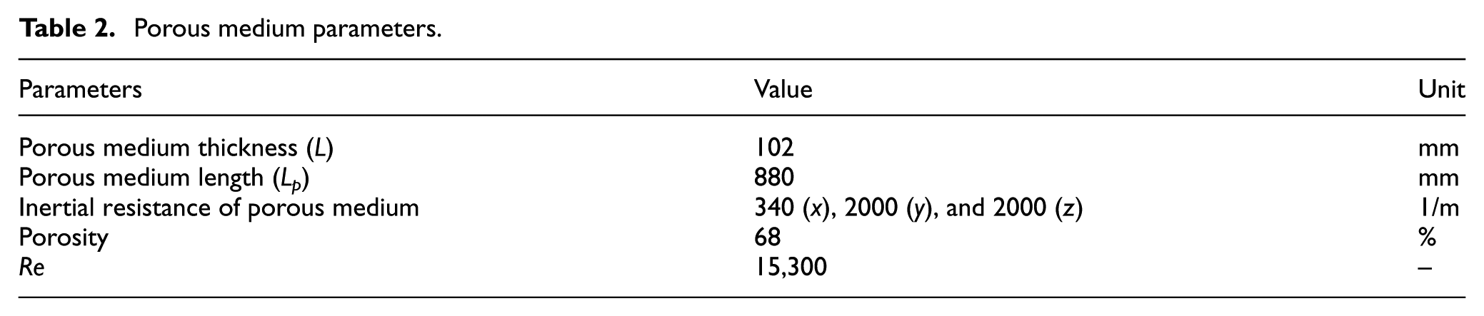
As stated above, porosity refers to the volume fraction of porous medium fluids in the porous medium domain. It usually influences source terms of chemical reactions and the body force in the application of porous medium model in chemical engineering practice. In this study, adequate attention is paid to the validity and the reliability of flow simulations. Based on the theoretical study and the numerical test on the impacts of porous medium parameters on flows, flow pattern in porous media has been achieved to approximate the steady turbulent flow without obvious vortex in the region perpendicular to the flow direction. Parameters in the porous medium domain are obtained as in Table 2 and Figure 3.

Table 2.

Porous medium parameters.

Parameters	Value	Unit
Porous medium thickness (L)	102	mm
Porous medium length (L_p)	880	mm
Inertial resistance of porous medium	340 (x), 2000 (y), and 2000 (z)	1/m
Porosity	68	%
Re	15,300	–

Figure 3.

Porous medium domain with vertical tube.

Initial boundary conditions and grid partitioning

Boundary conditions

A finite volume method was applied for discretization of the fluid governing equations, and a central difference scheme was utilized for the convective and the diffusion terms.

Two different “pressure boundary” conditions were specified at the inlet in the two cases, with P = 15,000 and 32,500 Pa, respectively. At the outlet, 0 Pa was applied by connecting atmosphere. A no-slip condition was applied at all solid walls. A “dynamic rotor” model was used for the thrust bearing, which rotated around the x-axis at 3000 r/min.

The fluid medium is set as water at 30°C. Numerical simulations on the coupling field between converged flow field in the motor and the porous medium domain were performed. Porous medium flow parameters were calculated and verified by permeability resistance coefficient (mainly involves inertial resistance coefficient) = 340, 2000, and 2000 m⁻¹ along three directions of the Cartesian coordinate system, and porosity ε = 0.68.

Grid partition

Reasonable grid distribution can facilitate the capture of the flow characteristics in narrow gaps, hydrodynamic bearings, distributary pipes, and the porous medium domain, thus enabling the subsequent analysis on axial and radial forces. Therefore, the computational domain for the flow field in the motor was not oversimplified, even though the full flow field grid scale is controlled. To maintain a satisfactory computational accuracy while considering the coupling between the gap flow and the large-scaled hydraulic structure, a hexahedron structural grid partition was applied.

Due to the large number of grids and limited length of the article, only the grid partition of the inlet channel is introduced. The overview of the 6,895,000 grids is shown in Figure 4(f). ICEM mesh quality checking is applied to calculate the skewness of each hexahedron. Skewness equals to 1 corresponds to an ideal hexahedral unit, and skewness equals to 0 corresponds to a reverse structure with a negative volume. In our study, skewness of 0.28% grids ranges between 0.4 and 0.6, and skewness of 97.5% grids is over 0.8, indicating a high grid quality. This offers a good preprocessing support to a clear capture of the flow field. y+ of the first layer grids has a mean value ranging from 82 to 100. The grid partitioning process of the inlet channel is shown in Figure 4(a)–(e). The inlet channel is first divided into eight central symmetric structures with 45° central angles. Y\O, L\O, and C\O grid strategies were used as in Figure 4(a)–(c), respectively. Subsequently, this grid partition (Figure 4(d)) was copied along the circumferential direction after passing the mesh quality check, thus forming an integrated gridding structure of the inlet pipe. Overlapped interfaces were set to be an internal wall to ensure the integration of the grid partitioning. An appropriate grid density distribution was selected to ensure a gradual transition in the parts with large variation of geometric sizes. To prevent grid stretching and shearing deformation, different node distributions, for example, hyperbolic and exponential (corresponding control parameters were given under different geometric sizes and variation of grid nodes), were applied.

Figure 4.

Grid partition strategy and plots: (a) L\Y\O grid strategy, (b) C\O grid strategy, (c) C\O grid strategy, (d) interior wall and interface, (e) section view of inlet channel, and (f) grid plots of motor.

To study the internal flow circulation in the motor coupled with porous media, the important role of the number of grids in the calculation accuracy, convergence, and computing resources need to be evaluated. The grid independent test was carried out with four grid systems, with the number of hexahedral cells of 2,078,000; 5,763,000; 6,895,000; and 10,500,000; respectively. The variation of the flow rate on the outlet is treated as the criterion of grid independence test. The final total number of grids is determined as 6,895,000 with less 1.15% of flow rate variation at the outlet, and the details of the grid distribution are listed in Table 3. Performances under two working conditions (Case 1 and Case 2) were compared. The convergence criterion in this study is that the relative residuals of velocities are less than 0.0001. Numerical results of the major flow field parameters are listed in Table 4. Case 1 and Case 2 have different inlet pressures. The total inlet pressure is 15,000 Pa in Case 1 and 32,500 Pa in Case 2. The outlet pressure in both cases is 0. ΔP is the inlet–outlet static pressure drop across the thrust bearing. P_Q and G_Q are the flow rate in the porous medium domain and the gap between the rotor and the stator, respectively. Gap Q/Porous Q is the ratio between the flow rate in the gap between the rotor and the stator, and the flow rate in the porous medium domain.

Table 3.

Grid distribution.

Region	Number of grids
Inlet	1,000,427
Thrust bearing	901,330
Transition region after Thrust bearing	2,374,064
Hydrodynamic bearing	995,406
Porous medium	180,576
Water gap	735,504
Hydrodynamic bearing and outlet	708,514

Table 4.

Comparison of two cases.

Case	Inlet pressure (Pa)	Outlet pressure (Pa)	ΔP (thrust bearing) (Pa)	P_Q (kg/s)	G_Q (kg/s)	Gap Q/Porous Q (%)
1	32,500	0	67,625	11.34	0.1146	1.0
2	15,000	0	67,562	11.06	0.1115	1.0

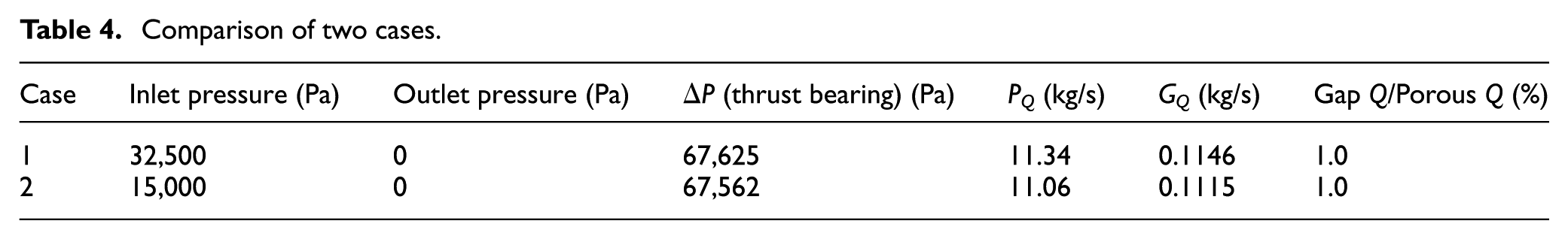
It can be concluded from Table 4 that between Case 1 and Case 2, the decrease in the pumping pressure of the thrust bearing is almost the same. The relative error of the flow rate in the porous medium domain is smaller than 2.4%, and the relative error of Gap Q/Porous Q is smaller than 2.7%. The flow rate of the gap between the rotor and the stator is 1% of the one in porous medium domain.

Results and analysis

Pressure distribution

The pressure distribution on the meridian plane of the motor for Case 1 is shown in Figure 5. The highest pressure is at the downstream of the outlet pipe of the thrust bearing. Fluid flows through all downstream parts and finally is discharged from the outlet pipe of the motor. Meanwhile, the pressure decreases to atmospheric pressure.

Figure 5.

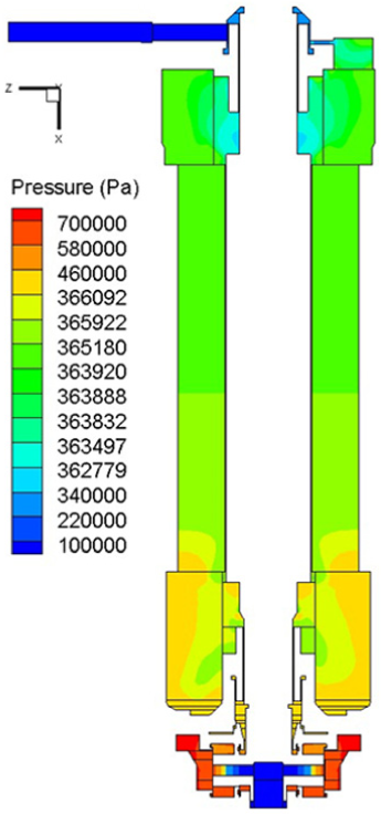
Pressure distribution on the meridian plane of the motor.

The pressure distributions on the inlet channel of the motor, the inlet pipe of the thrust bearing, and the meridian plane of part (3) for Case 1 are shown in Figure 6. Pressure reaches the maximum value (748,117 Pa) after the fluid flows through the thrust bearing. When fluid flows through the narrow gap in part (3), the pressure is decreased to 395,064 Pa at the outlet of part (3). It is the region with the maximum drop of pressure close to the thrust bearing. The variation in static pressure of main parts of the motor is listed in Table 5.

Figure 6.

Pressure distribution in the inlet channel of the motor and the thrust bearing.

Table 5.

Variation in static pressure.

Region	ΔP (Pa)
Inlet	−5126
Thrust bearing	67,562
Transition region after thrust bearing	−353,053
Hydrodynamic bearing	−28,778
Stator rotor and porous medium	−2209
Hydrodynamic bearing and outlet	−363,969

The pressure distribution on the radial section of the thrust bearing for Case 1 is shown in Figure 7. The maximum pressure is 679,259 Pa and the static pressure drop is 67,562 Pa. Pressure distribution on the radial section of the thrust bearing is similar to that of a pump impeller. It increases gradually from the shaft center to circumferential places. This is in accordance with the pumping effect of the thrust bearing in the whole motor.

Figure 7.

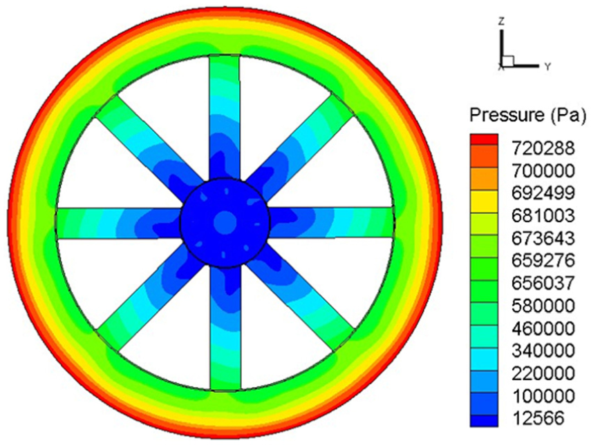
Pressure distribution in the thrust bearing (x = 0.2 m).

Flow field and local flow pattern

Flow on the meridian plane of the motor for Case 1 is shown in Figure 8. After entering the inlet channel, fluid is pumped by the thrust bearing to part (3) and flows through the hydrodynamic bearing, porous medium domain, and hydrodynamic bearing in the vicinity of the outlet pipe successively. Finally, it is discharged from the outlet pipe. An obvious vortex is captured at the left side in the external housing of the hydrodynamic bearing successfully. Besides, there is an obvious vortex on the upstream interface of the porous medium domain close to the shaft, which is caused by the large resistance coefficient of the porous medium domain, large resistance gradient on the interface between the porous medium inlet and the hydrodynamic bearing. Moreover, several vortices with different sizes and strengths are formed in the positions with small geometric size and large geometric gradient in the transition region between the thrust bearing and the hydrodynamic bearing. Two vortices are observed at the shaft side close to the outlet pipe.

Figure 8.

Streamlines on the meridian plane.

In Figure 9, fluid is pumped by the thrust bearing and flows downward along the axial direction. However, some small vortices locating in the large housing close to the inlet channel are captured. A certain reverse velocity gradient exists in the circumferential wall, forming local vortices.

Figure 9.

Streamlines in inlet channel and thrust bearing.

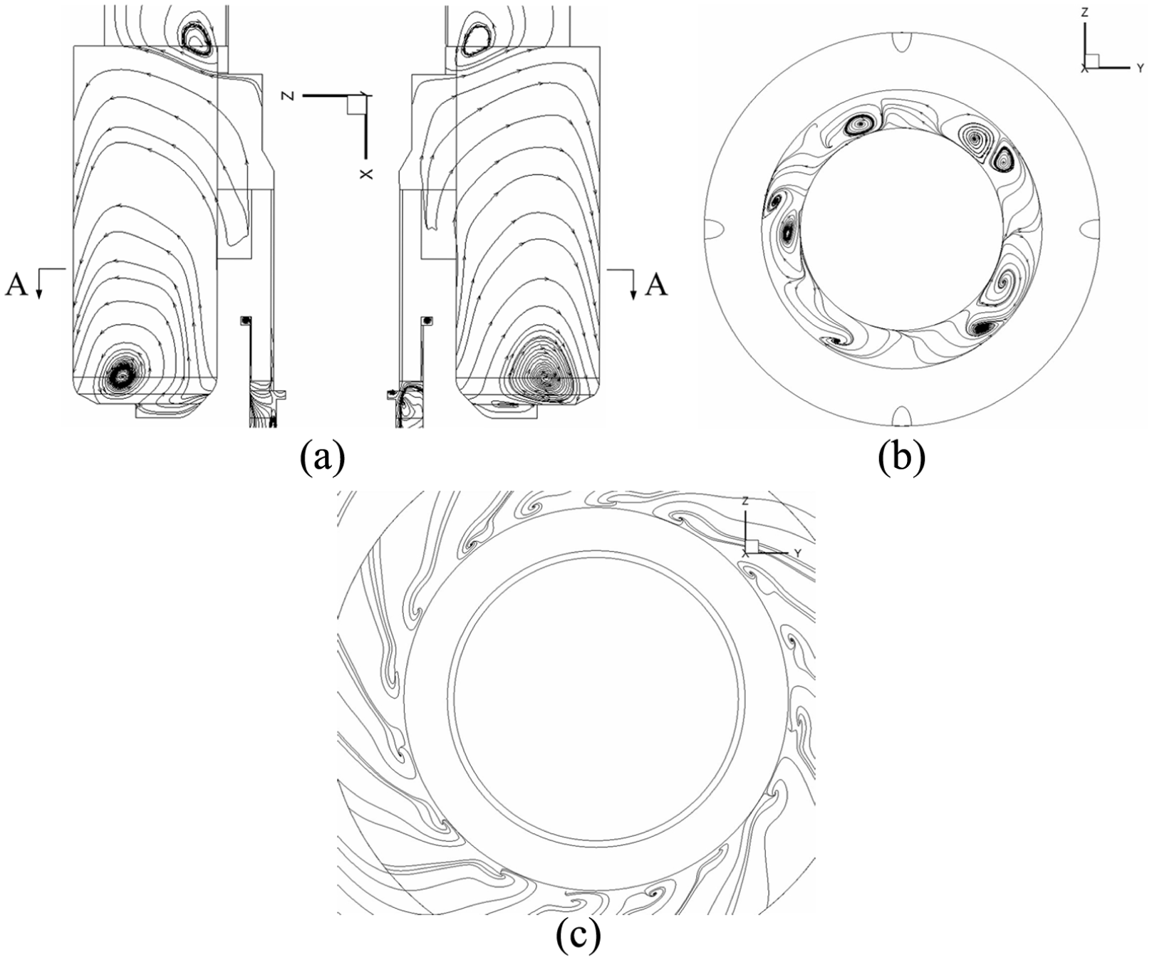
Radial flow distribution on the radial sections of the main and vice thrust pads of the thrust bearing, as well as the thrust bearing are shown in Figure 10. Two unsymmetrical vortices are formed in each housing chamber, close to the radial inlet and outlet pipes of the housing. Moreover, vortices with different strengths are formed in the ring channel connected to the radial inlet pipe of the housing. The vortex at the inlet of the radial thrust bearing channel is shown in Figure 10(b). This vortex is symmetric around the rotation center and is formed by the high-speed rotation of the shaft and local differences in pressure and velocity. The flow field on the radial section of the vice thrust pad of the thrust bearing is shown in Figure 10(c). Different from that on the main thrust pad, fluid is driven by a high-speed pumping of the thrust bearing and forms vortices with different size in the local housing which is symmetric around the radial distribution center. These vortices concentrate at the radial outlet of the housing. The amplified flow field in the gap between two coaxial cylinders close of the vice thrust pad close to the shaft is shown in Figure 10(d). Fluid in the gap between the external side and the inlet of housings form several vortices by the high-speed rotation of the shaft. Size of this radial gap can influence the number of vortices.^16,17 The comparison of the predicted number of Taylor vortices between references and the present paper is listed in Table 6. The number of Taylor vortices in this study is different compared with those in the references, due to the difference between Re and Ta. Moreover, some vortices asymmetric around the shaft center with different strengths are formed in the large ring gap at the internal side, which accelerates hydraulic loss of the fluid in the gaps.

Figure 10.

Local flow in thrust bearing (radial section): (a) flow in the vice thrust pad of the thrust bearing near of the inlet, (b) flow in the inlet of the main pad of the thrust bearing, (c) flow in another vice thrust pad of the thrust bearing, and (d) flow in the gap between two coaxial cylinders near of the shaft.

Table 6.

Comparison of the number of Taylor vortices.

	Qin¹⁶	Peng et al.¹⁷	This study
Re	6 × 10⁴	130	1.5 × 10⁴
Ta	2.28 × 10⁵	5 × 10⁵	3.1 × 10⁷
Length of the gap (mm, axial)	400	150	11
Width of gap (mm, radial)	12.7	10	12.5
Number of Taylor vortices (pairs)	6	15	2

In the spatial flow distribution in the thrust bearing and local amplification (Figure 11), flow on the bearing cage surface is symmetric around the axial section of the bearing center and extends toward the external side of the bearing cage. Flow in the bearing cage is circumferential flow in the space and enters as a rotational flow into the bearing cage from the upstream of the thrust bearing and then is pumped to the vice thrust pad. The second image in Figure 11 is the circumferential circulation flow of fluid in the bearing ring.

Figure 11.

Spatial flow distribution in the thrust bearing.

Streamlines in the transition region between the thrust bearing and the sliding bearing are illustrated in Figure 12(a) and (b). After flowing through two layers of gaps and the local amplified middle channel, several vortices are formed at the position of circumferential gap channel with large geometric deformation and in the gap channels distributed along the circumferential direction. The flow field in the distributary pipe center is shown in Figure 12(c) and (d). In Figure 12(d), there is one vortex in the circumferential gap channel at the distributary pipe inlet close to the external side, caused by different flow velocities and directions of rotations, and the other two vortices in the circumferential gap channel at the distributary pipe inlet close to the internal side are captured, due to the difference of flow velocities in the distributary pipe inlet and flow velocities in the gap connected to the distributary pipe. Flow patterns of the radial section of the distributary pipe are shown in Figure 12(e), with three vortices with different sizes.

Figure 12.

Flow distribution in part (3): (a, b) flow in the transition region between the thrust bearing and the sliding bearing, and (c, d, e) flow in the distributary pipe.

The flow in the hydrodynamic bearing close to the motor inlet is shown in Figure 13(a). There are some vortices in the upstream of the large external radial channel and a number of vortices in the corners (Figure 13(b)). Two vortices close to the center of rotation are captured on the interface between this channel and the porous medium domain, which is related to the permeability and the inertial resistance of the porous medium. The streamlines on radial section A-A is shown in Figure 13(c). Many vortices symmetric around the shaft center are observed close to the center of rotation.

Figure 13.

Flow distribution in the hydrodynamic bearing: (a) flow in the hydrodynamic bearing and outer chamber near of the inlet, (b) flow in the outer chamber of the hydrodynamic bearing near the inlet on the radical section, and (c) A-A section in sub-Fig. (a).

Spatial flow in the gap between the rotor and the stator is shown in Figure 14. Flow in this gap is the rotational flow from the upstream. Due to the high-speed rotation of the shaft, there is rotational flow around the shaft in the gap between the rotor and the stator. Finally, fluid flows toward the downstream through the gap outlet.

Figure 14.

Flow distribution in the gap between the rotor and the stator.

The flow in the porous medium is illustrated in Figure 15. Since the inertial resistance coefficients of porous medium in three directions of the Cartesian coordinate system are set as 340, 2000, and 2000, respectively, fluid flow in the porous medium is regular without obvious vortices. However, the flow close to the shaft at the inlet and outlet of the porous medium domain is disordered. This conforms to the pressure distribution and flow patterns in Figures 7 and 12, respectively. There is a circumferential rotational flow in porous medium which overcomes the inertial resistance at the inlet.

Figure 15.

Flow distribution in the porous medium.

The flow in the hydrodynamic bearing and the outlet pipe is shown in Figure 16. In Figure 16(a), axisymmetric vortices are observed in both inlet and outlet of the hydrodynamic bearing, and some vortices are captured at top of motor outlet. Figure 16(b) displays the flow pattern in the outlet pipe. Two vortices with different sizes and strengths are formed at different positions close to the connection between the entrance of the outlet pipe and circumferential channel at the axis side, caused by asymmetric flows in the outlet pipe along the axial direction and the circumferential direction. There is no complete circulation loop of fluid in the whole model. Instead, fluid can only flow through certain vortices and partly return to the outlet pipe. Flow in the local circumferential gap close to the outlet pipe is presented in Figure 16(c). There are four housings, accompanied with irregular flow distributions. Two vortices are predicted in the connection hole between two gap flows, which might be related to the uneven distribution of flows in the external circumferential housings.

Figure 16.

Flow distributions in the hydrodynamic bearing and the outlet pipe: (a) flow in the hydrodynamic bearing near the outlet, (b) flow in the outlet pipe, and (c) flow in the local circumferential gap near the outlet pipe.

Typical vortex analysis

The data of flow field are transferred to dimensionless value so that the number of variables in the problem is reduced. Reynolds number Re encapsulates the rotor speed and the machine size.

Taylor vortex

Considering the parallel and non-parallel gap flows in the vicinity of the canned motor shaft region, in the case of inertial instability as Taylor–Couette flow,^18–20 in different parts and geometries of the canned motor, when the Taylor number exceeds a critical value, inertial (Taylor) instabilities arise, which may lead to Taylor vortices or cells.^21–23 In this article, Taylor number is calculated according to

Ta = \frac{Ω^{2} R_{1} {(R_{2} - R_{1})}^{3}}{υ^{2}}

(7)

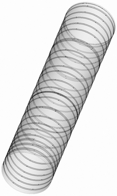
where Ω is a characteristic angular velocity; R₁ and R₂ are the radii of the internal and external cylinders, respectively; and $υ$ is the kinematic viscosity. Note that Ta_c (∼1700) is the critical Taylor number when the state of flow from laminar transit into turbulent.

Taylor vortices in the parallel gaps close to the inlet of part (4) are shown in Figure 17. The length of these gaps along the flow direction is 6.85 mm and the radial gap is 7.5 mm. Figure 17(b) presents the distribution of Taylor vortices, where Re = 3.44 × 10⁴ and Ta exceeds the critical value, reaching 7.69 × 10⁷. Figure 17(c) is the three-dimensional (3D) distribution of Taylor vortices in the gaps, which shows that Taylor vortices are symmetric in the circumferential direction and flow in from the upstream and flow out from the downstream.

Figure 17.

Location and morphology of Taylor vortices in the vicinity of part (4): (a) the gap near the distributary pipe of part (4), (b) flow in the gap of the sub-Fig. (a) on the axial section, and (c) flow in the gap of the sub-Fig. (a).

Taylor vortices in the non-parallel gaps in part (3) are shown in Figure 18. Figure 18(a) is the geometric structure of gaps. Re = 2 × 10⁴, and Ta exceeds the critical value, reaching 3.1 × 10⁷. Figure 18(b) is the distribution of Taylor vortices. Since there is a distributary pipe on the circumferential direction connected with the ring disk gap in the external side, Taylor vortices are not strictly circumferentially symmetric in the region close to this distributary pipe. The 3D spatial distribution of three Taylor vortices (green dotted line) with a similar pattern and size in the side far away from the distributary pipe is displayed in Figure 18(c). These three Taylor vortices are circumferentially symmetric. The 3D spatial distribution of Taylor vortices (green dotted line) with different patterns and sizes in the side close to the distributary pipe (black circle) is illustrated in Figure 18(d). It is corresponding to the asymmetry of Taylor vortices in the meridian plane in Figure 18(b). The 3D structure of this part is described in Figure 18(e), and the red part represents the distributary pipe.

Figure 18.

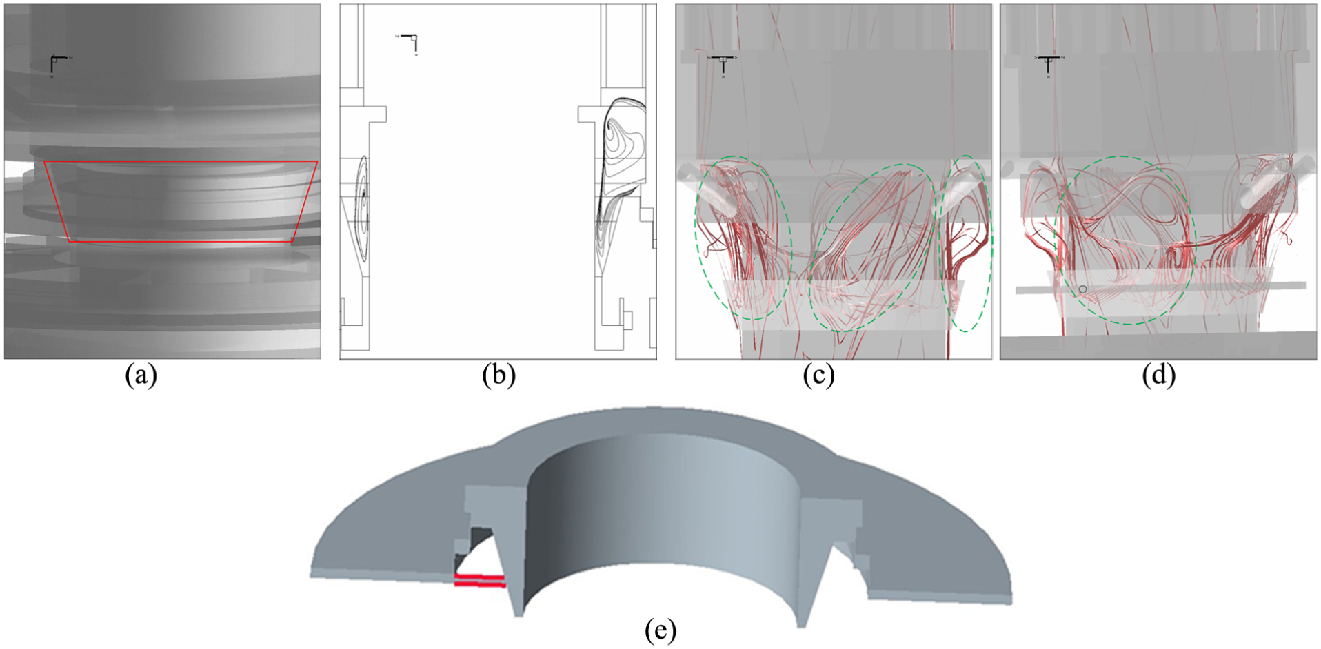
Location and morphology of Taylor vortices in part (3): (a) transition region after the thrust bearing, (b) flow in the transition region after the thrust bearing on the axial section, (c, d) flow in the transition region after the thrust bearing, and (e) spatial structure of the distributary pipe of the transition region after the thrust bearing.

Dean vortex

A similar instability, that is, Taylor–Dean flow, occurs in the circulation flow in the canned motor through a (quasi) curved channel when drove by a stream-wise pressure gradient.^24,25 Flow instability will occur when Dean number

Dn = \frac{G d^{3}}{μ υ} \sqrt{\frac{2 d}{R}}

(8)

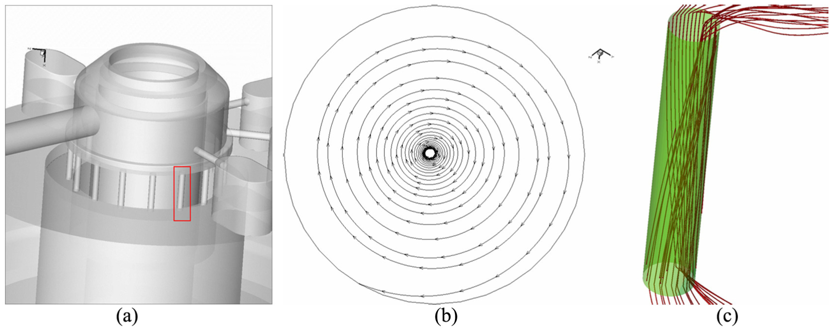
exceeds a critical value, where G stands for the pressure gradient along the stream-wise and is taken to be positive, d is the half width of the pipe corner, $μ$ is the viscosity, $υ$ is the kinematic viscosity, and R is the radius of the curvature of the centerline of the pipe. Re is Reynolds number based on the mean velocity of the unperturbed flow.^26,27 In view of the complex structures, Reynolds number and corresponding Taylor number, Dean number, and relative vortices appear in the flow field of the canned motor.

Dean vortices in 1 of the 20 distributary pipes (red rectangle in Figure 19(a)) in a uniform distribution circumferentially in part (4) are shown in Figure 19. In Figure 19(b), there is one pair of approximately symmetric opposite Dean vortices in the radial section of the distributary pipes. The spatial distribution is presented in Figure 19(c). Fluid forms two rotational flows in the distributary pipes and finally moves toward the downstream. Where the static pressure drop between inlet and outlet of the distributary pipes ΔP (Pa) = 2600, Reynolds number in the pipes Re = 3.65 × 10⁴, and Dean number Dn = 5771.

Figure 19.

Location and morphology of Dean vortices in part (4): (a) spatial structure of the distributary pipes in part (4), (b) flow in the distributary pipe in red rectangle in sub-Fig. (a) on the radical section, and (c) flow in the distributary pipe in red rectangle in sub-Fig. (a).

Dean vortices in 1 of the 20 distributary pipes (red rectangle in Figure 20(a)) in a uniform distribution circumferentially in part (7) are shown in Figure 20. In Figure 20(b), there is only one Dean vortex in the radial section of the distributary pipes. The spatial distribution of this Dean vortex is shown Figure 20(c). Fluid forms one rotational flow in the distributary pipes and finally leaves the distributary pipes to downstream. Corresponding non-dimensional parameters are Re = 4.485 × 10⁴, Dean number Dn = 7340, and the variation of the static pressure ΔP is 3.495 × 10⁴ Pa.

Figure 20.

Location and morphology of Dean vortices in part (7): (a) spatial structure of the distributary pipes in part (7), (b) flow in the distributary pipe in red rectangle in sub-Fig. (a) on the radical section, and (c) flow in the distributary pipe in red rectangle in sub-Fig. (a).

Local hydraulic loss analysis

Energy partition

Energy partition in the canned motor can be summarized as follows: the input energy of the canned motor consists of pressure energy given by inlet boundaries and the rotating mechanical energy provided by the rotating thrust bearing. These energies are converted into the mechanical energy (the kinetic energy, the gravitational potential energy, and the pressure energy) of the mean flow and the hydraulic losses (the turbulent kinetic energy and the internal energy). Pressure distribution in the flow field, especially in the narrow gap flow surrounding the shaft and the viscous forces in the boundary layer surrounding the shaft, will impact on the radial and the axial shaft forces. In the meantime, the turbulent kinetic energy has some influence on the pressure distribution and flow field distribution through the turbulent cascade (the dotted line). The internal energy has not been considered in this article yet. On this basis, the influence of each factor on shaft forces was analyzed in detail in this article. The relative energy conversion processing is shown in Figure 21.

Figure 21.

Relationship between energy conversion and shaft forces in the canned motor.

Energy balance equation

According the method described by Wilhelm et al.,²⁸ the total hydraulic losses of the canned motor evaluated by RANS model are influenced finally by follow terms

\begin{matrix} gQ Δ H & = \int \int_{S_{in}} (\frac{\bar{P *}}{ρ g} + \frac{1}{2 g} \bar{u_{i}} \bar{u_{i}}) g \bar{u_{x}} dS - \int \int_{S_{out}} (\frac{\bar{P *}}{ρ g} + \frac{1}{2 g} \bar{u_{i}} \bar{u_{i}}) g \bar{u_{z}} dS \\ = \underset{A}{\underset{︸}{- \int \int_{S} (2 \bar{u_{i}} (v \bar{S_{ij}} + \bar{v_{t} S_{ij}}) n_{j}) dS}} + \underset{B}{\underset{︸}{\int \int_{S} (\bar{u_{i}} ({\bar{u_{i}}}^{'} {\bar{u_{j}}}^{'})) n_{j} dS}} \\ + \underset{C}{\underset{︸}{\underset{V}{\int \int \int} 2 v \bar{S_{ij}} \bar{S_{ij}} dV}} + \underset{D}{\underset{︸}{\underset{V}{\int \int \int} - ({\bar{u_{i}}}^{'} {\bar{u_{j}}}^{'}) \bar{S_{ij}} dV}} + \underset{E}{\underset{︸}{\underset{V}{\int \int \int} 2 (\bar{v_{t} S_{ij}}) \bar{S_{ij}} dV}} \end{matrix}

(9)

where S_in is the inlet and S_out is the outlet of the canned motor, u_i is the velocity in x_i direction, and ${\bar{u}}_{i}$ stands for the time-averaged value of u_i, $\bar{P *}$ is the modified time-averaged value of static pressure, $v$ is the fluid kinematic viscosity, $v_{t}$ is the turbulent viscosity, $n_{j}$ is the jth component of the outer-pointing normal, and ${\bar{S}}_{ij} = 1 / 2 (\partial {\bar{u}}_{i} / \partial x_{j} + \partial {\bar{u}}_{j} / \partial x_{i})$ is the strain rate tensor. The related variables in equation (9) are obtained in CFD-post platform. Terms (A) and (B) correspond to the diffusion of the mean kinetic energy, term (C) is the viscous dissipation of the mean kinetic energy. The turbulent kinetic energy production is presented by terms (D) and (E). To be specific, (D) is resolved and (E) is modeled part which involves the turbulent viscosity ν_t.

In equation (9), Terms (A) and (B) can be neglected for corresponding flow patterns due to their quite small contribution to the energy balance. Terms (D) and (E) can be evaluated by $P_{D} = \int \int \int_{V} - ({\bar{u_{i}}}^{'} {\bar{u_{j}}}^{'}) \bar{S_{ij}} dV$ and $P_{E} = \int \int \int_{V} 2 (v_{t} \bar{S_{ij}}) \bar{S_{ij}} dV$ , respectively, and $P_{C} = \int \int \int_{V} 2 v \bar{S_{ij}} \bar{S_{ij}} dV$ indicates the viscous dissipation of the mean kinetic energy.

The contribution of P_C, P_D, and P_E to the hydraulic loss (gQΔH) for Case 1 is illustrated in Figure 22. It is noted that the part of the viscous dissipation P_C in the hydraulic losses is relatively small (13.14% of the total hydraulic loss). The production of turbulent kinetic energy (sum of P_D and P_E) is the main contribution to the hydraulic losses in the canned motor. Comparing to the P_E, the value of P_D is quite small. The evaluation of the hydraulic losses is thus more dependent on the turbulence model in the RANS simulation.²⁸ RNG k-ε turbulence model is applied in predicting the flow in the motor presented in this article, which has a good performance in simulating flow with various vortices, high strain rates, and wavy streamlines.²⁹ In the simulations of this article, the turbulent flow is nearly totally modeled, and that is corresponding to the large value of P_E.

Figure 22.

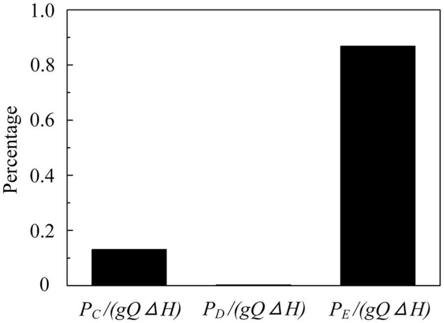
Contribution of P_C, P_D and P_E to the hydraulic loss (gQΔH) for Case 1.

Local hydraulic loss analysis in the canned motor for Case 1

On the local hydraulic loss of the vertical shaft, R Padulano and colleagues^30,31 investigated the hydraulic features of a vertical drop shaft through experiments and given the limited attention in hydraulic structure under transitional and weir flow. In this article, hydraulic losses of circulation flow in the canned motor are mainly related to the turbulent kinetic energy production, which is principally modeled in RANS. In order to identify the hydrodynamic features responsible for turbulent production and hydraulic losses in the canned motor, distribution of P_E for the RANS simulation is shown in Figure 23 for Case 1. High value of P_E is captured in the channel close to the main thrust pad of the thrust bearing, which is in agreement with flow structures in Figure 10(a) well. Pressure on part (2) corresponds to a strong local flow structure (circulation flow (Figure 11)). Pressure on part (3) is subject to drastic change of geometric structures and a high-speed rotation of the shaft, which is in accordance with flow patterns in Figure 12. Pressures on part (4), part (7), and part (8) are related to a high-speed rotation of the shaft and the thin thickness of hydraulic film in the hydrodynamic bearing. Large value of P_E on the outlet pipe is due to the vortices in the outlet pipe (Figure 16(b)).

Figure 23.

Distribution of P_E on the median plane in the canned motor for Case 1.

Figure 24 shows the distribution of P_E on a plane, and its location is determined by the dotted lines in Figure 23. P_E on the hydraulic film of the hydrodynamic bearing, and the internal and external walls of the external housing are relatively high, caused by the high-speed rotation of the shaft, the thin thickness of the hydraulic film in the hydrodynamic bearing, vortices on the internal wall of the external housing (Figure 13(c)) and strong circulation flow on the external wall.

Figure 24.

Distribution of P_E on a plane perpendicular to the x-axis in the canned motor.

P_E profiles in Figure 25 obtained through azimuthal averaging on the plane which is calibrated by the dotted lines in Figure 23. The maximum values of P_E are calculated in the hydrodynamic bearing (R/R_max = (0.24, 0.25)) and the walls of the housing out of the hydrodynamic bearing (R/R_max close to 0.32 and 1).

Figure 25.

P_E on a plane perpendicular to x-axis in the canned motor.

The right-hand side of equation (9) is calculated over a control volume V located between the inlet (x = 0) and an arbitrary x plane. The hydraulic losses as a function of dimensionless variable x/x_max for Case 1 are illustrated in Figure 26. It is worth emphasizing that Figure 26 corresponds to the cumulated value of the hydraulic losses between the origin x = 0 and a given x location. A dramatic increase in the hydraulic loss is observed in the canned motor parts (2) and (3) and the latter part of (7) and (8) (x/x_max = (0.03, 0.23), (0.87, 1)). However, the increase in the hydraulic loss in the canned motor parts (1), (4), (5), and (6) is slower than the previous parts. The fluctuation of the different components of hydraulic losses along the whole shaft is shown in Figure 26, which is hard to measure systematically by experiment at present. The relatively reasonable prediction of the downstream flow field provides information for hydraulic loss analysis. Figure 26 furthermore shows that the flow mechanism of the hydraulic loss in different parts of the canned motor is quite different.

Figure 26.

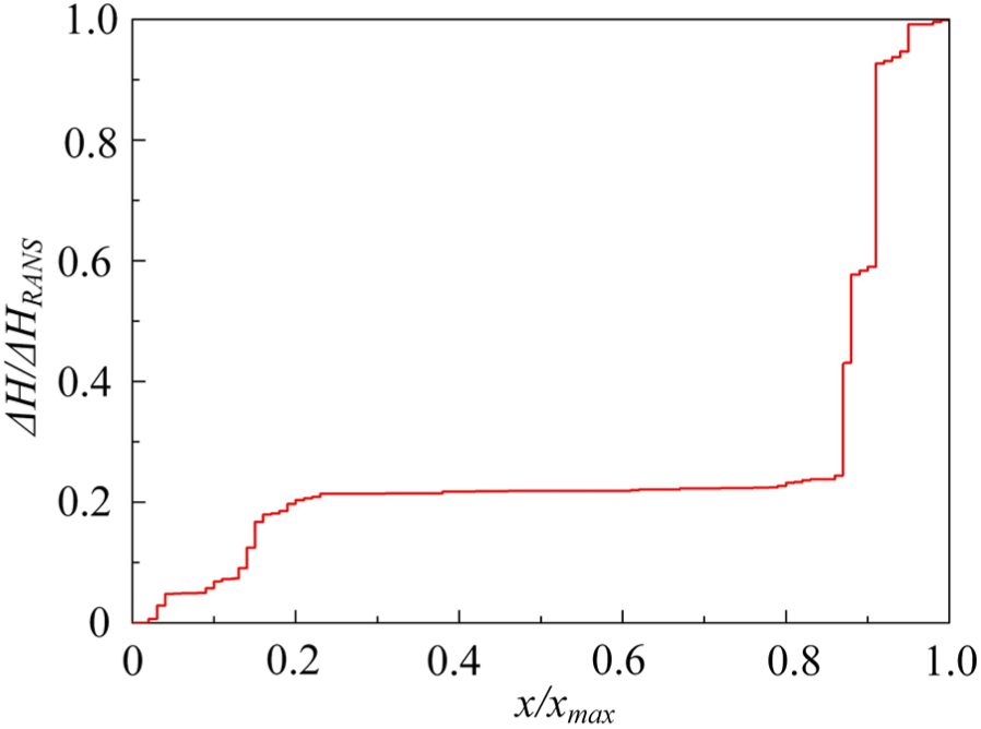
Local hydraulic loss (Case 1).

Shaft forces

Previous research of axial forces has neglected small-scale geometric structures and gap flows on the radial direction which can influence the axial force to some extent. In this article, the corresponding influence mechanism was analyzed, and internal turbulent flow patterns were calculated and captured from the perspective of hydromechanics based on the non-simplified hydraulic geometry of the motor. On this basis, shaft forces were analyzed combined with hydraulic loss.

In Figure 27, the ratio between shaft size along the flow direction and the total shaft length is used as the x-axis, and radial force at different shaft positions is set as the y-axis. The black solid line is the radial force caused by uneven pressure distribution. The red dotted line is the radial force along the definition coordinates of the shaft caused by fluid viscosity. The green dotted line is the total radial force along the x-axis direction which is caused by uneven pressure distribution and fluid viscosity force. The radial force along the x-axis direction which is caused by fluid viscosity force is very small and can be neglected compared to the radial force caused by uneven pressure distribution. However, the uneven pressure distribution along the radial direction caused by gap flows leads to an uneven distribution of the radial forces. On part (3), two obvious fluctuations of radial force near x_shaft/x_{shaft_max} = 0.03255 compared to in vicinity of the numerical value are formed by large gap flows and single distributary pipe, which conforms to high hydraulic loss in corresponding positions in Figure 23. With the increase in the x-axis value, radial force close to the downstream of hydrodynamic bearing fluctuates more than near radial forces, which is attributed to the great radial gradient of geometric size and strong resistance at inlet of the porous medium domain, which conforms to high hydraulic loss in corresponding positions in Figure 23. The strongest radial forces (x_shaft/x_{shaft_max} = 0.9772) are on part (7) and part (8). This is mainly because there is only one outlet pipe on the circumferential direction of the motor. High hydraulic losses in part (7) and part (8) are corresponding to complicate vortices. Uneven circumferential distribution of these complicated vortices is the main cause of local extremes of radial forces. Besides, the double dot red line stands for the radial force computed by the empirical formulae in relevant Shenyang Pump Research Institute,³² Guan,33 and Konno and Ohno³⁴ in Figure 27. The radial force on the shaft along the x-axis consists of the variation of P in outlet pipe, and the dynamic resisting force R of the five outer housings in the vicinity of the outlet

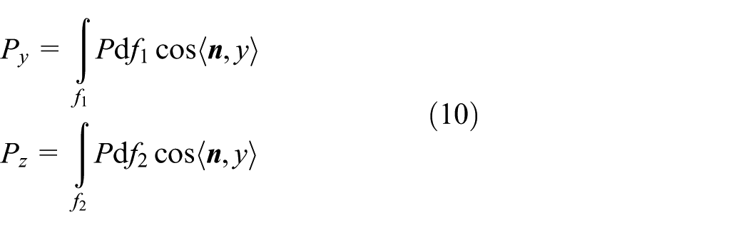
\begin{matrix} P_{y} = \int_{f_{1}} P d f_{1} \cos 〈 n, y 〉 \\ P_{z} = \int_{f_{2}} P d f_{2} \cos 〈 n, y 〉 \end{matrix}

(10)

where P_y and P_z are the variation of P in the outlet pipe in y and z directions, respectively. n is the normal; $f_{1}$ and $f_{2}$ are the projections of outlet section in y and z directions, respectively

\begin{matrix} - R_{y} = \int_{f_{4}} ρ u_{ny} d f u \cos 〈 n, y 〉 - \int_{f_{3}} ρ u_{ny} d f u \cos 〈 n, y 〉 \\ - R_{z} = \int_{f_{4}} ρ u_{nz} d f u \cos 〈 n, y 〉 - \int_{f_{3}} ρ u_{nz} d f u \cos 〈 n, y 〉 \end{matrix}

(11)

where R is the dynamic resisting force; $ρ$ is the fluid density; $u_{ny}$ and $u_{nz}$ refer to the velocity of distribution pipes of the outer housings in y and z directions, respectively. u is the velocity in x direction; $f_{3}$ and $f_{4}$ are the projection of the inlet and outlet sections of the housing in y and z directions, respectively.

Figure 27.

The evolution of the radial force on the shaft along x-axis in the canned motor.

The radial force calculated by the CFD code in this article is in good agreement with the one computed by the empirical formulae, and the maximum error is less than 6%, as shown in Figure 27. The double dot red line refers to the axial force caused by pressure, estimated by the empirical formulae in Shenyang Pump Research Institute,³² Guan,33 and Konno and Ohno.³⁴

In Figure 28, the ratio between shaft size along the flow direction and the total shaft length is set as the x-axis, and the axial force at different shaft positions is used as the y-axis. The black solid line is axial force caused by pressure action on the shaft, the red dotted line is axial force along the definition coordinates of the shaft caused by fluid viscosity force, and the green dotted line is the total axial force along the x-axis direction which is caused by the superposition of pressure and fluid viscosity force. The axial shaft force caused by uneven pressure distribution is smaller than the axial force caused by fluid viscosity force. Relatively stronger local axial forces are observed on part (3) and inlet of part (5), which are contributed by the widening of the channel (positive axial force) and porous medium resistance. The axial force along the x-axis which is caused by fluid viscosity force is relatively strong. Axial forces occur on part (3), and inlet and outlet of part (5), part (7), and part (8) fluctuate violently. Due to circumferential gap turbulent flows in these parts along the shaft and liquid film on the hydrodynamic bearing, these complicated 3D turbulent flows in narrow gaps not only cause huge hydraulic loss in corresponding parts (Figure 23) but also bring strong axial force caused by fluid viscosity. Moreover, the double dot red line refers to the axial force caused by pressure, which is computed by the empirical formulae in Shenyang Pump Research Institute,³² Guan,³³ and Konno and Ohno,³⁴ and it matches well with the results of simulation. The axial force on the shaft is mainly composed by the pressure P in the inlet (F₁) and the dynamic resisting force F₂ of the transition region after the thrust bearing

F_{1} = γ π (R_{2}^{2} - R^{2}) [\frac{1}{2} m {u_{in}}^{2} - (R_{2}^{2} - \frac{R_{2}^{2} + R^{2}}{2}) \frac{ω^{2}}{8 g}]

(12)

where $γ$ is the floatation of the fluid; $R_{2}$ and $R$ stands for the radius of the thrust bearing and shaft, respectively. $ω$ is the rotational speed of the shaft, and $u_{in}$ is the velocity in x direction of inlet

F_{2} = \frac{Q}{g} γ (u - v' \cos θ)

(13)

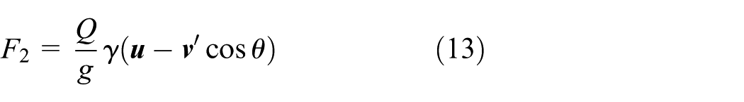
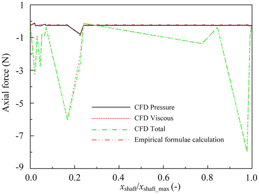
where Q is the flow rate; $γ$ is the floatation of the fluid; $u$ and $v'$ is the velocity of the inlet and outlet of the transition region after the thrust bearing, respectively; $θ$ is the angle between $v'$ with x-axis.

Figure 28.

The evolution of the axial force on the shaft along x-axis in the canned motor.

The calculation of the axial force on the shaft caused by viscosity is dependent on the relative resistance coefficients, which are usually determined by experiments. Hence, only the axial force caused by pressure is evaluated by the empirical formulae, as shown in Figure 28.

Histogram of the radial force caused by pressure P_Axial (black), axial force P_Radial (black); radial force caused by fluid viscosity V_Axial (red), axial force V_Radial (red); and total radial forces T_Axial (green), total axial forces T_Radial (green) is shown in Figure 29. P_Radial and V_Axial are as high as 271.67 and 19.32 N, respectively. T_Axial = 272.21 N and T_Radial = 19.63 N, indicating that the radial force is stronger than the axial force in the shaft system of canned motor.

Figure 29.

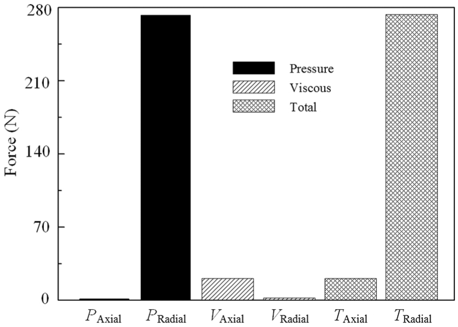
Forces of the shaft of the canned motor.

Proportions of the radial force and the axial force in total radial forces and total axial forces are presented in Figure 30. Obviously, P_Axial/T_Axial = 1.63% (black), which can be neglected compared to V_Axial/T_Axial= 98.37% (red). Due to related geometric structures (e.g. gap flows) on radial direction of the shaft, P_Radial/T_Radial = 99.8%, which suggests that the radial force caused by fluid viscosity can be neglected.

Figure 30.

Contribution of P_Axial, P_Radial, V_Axial, and V_Radial to the T_Axial, T_Radial for Case 1.

Moment (M) distribution at different positions along the shaft direction is shown in Figure 31. Great changes of M are observed at positions with violent fluctuations of radial force (Figure 26). The maximum shaft moments on part (7) and part (8) reach 131.99 N m. In addition, radial force changes greatly due to the radial flow gaps and single distributary pipe on part (3), which reflects large moment −M = 18.85 N m at the position (x_shaft/x_shaft__max = (0, 0.03255)).

Figure 31.

Distribution of moments on shaft along x-axis in the canned motor for Case 1.

Conclusion

In this article, the motor stator is approximately viewed as a porous medium domain. Ergun equation is used as the governing equation of the porous medium domain. The numerical results on the coupling field between flow in motor and porous medium flow are acquired based on the standard RNG k-ε turbulence model. Results demonstrate that the static inlet–outlet pressure increase in the thrust bearing reaches 67,562 Pa, which provides essential conditions for fluid to overcome downstream gravity and reduce hydraulic loss. However, the pressure declines sharply by 353,053 Pa after part (3). It is the region with the maximum pressure attenuation close to the thrust bearing.

With respect to flow in the motor, gap flow between rotor and stator of the motor is developed into strong rotational flow. This gap flow rate is 1% of flow in the porous medium domain. Axial symmetric vortices form at inlet between radial channels in the thrust bearing. In parallel gaps close to part (4), Re = 3.44 × 10⁴ and Ta = 7.69 × 10⁷, accompanied with circumferentially symmetric Taylor vortices. In the non-parallel gaps in part (3), Re = 2 × 10⁴ and Ta = 3.1 × 10⁷ due to the distributary pipe. Taylor vortices in approximately circumferential symmetric distribution are also formed here. In many distributary pipes outside two hydrodynamic bearings, Dean vortices are formed in two working conditions (Case 1: ΔP = 2600 Pa, Re = 3.65 × 10⁴, and Dn = 5771; Case 2: ΔP = 3.495 × 10⁴ Pa, Re = 4.485 × 10⁴, and Dn = 7.34 × 10⁴).

For the hydraulic losses of the canned motor, there is a strong increase in the P_E observed in the canned motor parts (2), (3), (7) and the latter part of (8)(x/x_max = (0.03, 0.23), (0.87, 1)). However, the increase in hydraulic losses in the canned motor parts (1), (4), (5), and (6) is slower than the previous regions. The results show that the vortices are quite complex due to complicated geometry and the corresponding dissipation is relatively high.

By combining hydraulic loss analysis, a strong increase in the radial force is predicted in the parts of (7) and (8) (x/x_max = (0.84, 0.97)), and axial force are captured in the parts (3), (5), and (7) of canned motor, respectively (x/x_max = (0.24, 0.17), (0.84, 0.97)). Shaft forces along the flow direction (axial direction) are mainly caused by fluid viscosity force, while shaft forces along the radial direction are mainly caused by pressure. The high-speed rotation of the shaft and the gap flow at the shaft surface generate strong turbulence, which not only caused non-uniform pressure distribution on the axial surface but also produced high hydraulic loss in local positions, thus developing high radial forces.

Footnotes

Handling Editor: Mustafa Canakci

Declaration of conflicting interests

The author(s) declared no potential conflicts of interest with respect to the research, authorship, and/or publication of this article.

Funding

The author(s) disclosed receipt of the following financial support for the research, authorship, and/or publication of this article: This work was supported by the National Natural Science Foundation of China (grant nos 51479196, 51179192, 51139007, and 51476083), the Program for New Century Excellent Talents in University (NCET) (grant no. NETC-10-0784), and State Key Laboratory of Hydro Science and Engineering (Open Research Project No. sklhse-2017-E-01).

References

Ding

Wang

et al . Flow analysis and optimization of port-plate centrifugal pump in electric motor pump. J Mech Eng 2009; 45: 199–205.

Young

LJ.

Lifetime evaluation of cracked shaft sleeve of reactor coolant pump under thermal striping. Int J Solids Struct 2001; 38: 8345–8358.

Zhang

Chen

Zhang

et al . Analysis of friction-induced vibration in a propeller–shaft system with consideration of bearing–shaft friction. Proc IMechE, Part C: J Mechanical Engineering Science 2014; 228: 1311–1328.

Liu

Kong

Daun

et al . Temperature field study of hot water circulation pump shaft system. IOP Conf Ser: Mat Sci 2016; 129: 012034.

Wang

Yao

HN.

Design of test bench for flyweel of the shaft-seal nuclear coolant pump and ANSYS analysis. Appl Mech Mater 2014; 644–650: 559–562.

Zuo

Liu

Fan

et al . Optimization of a centrifugal boiler circulating pump’s casing based on CFD and FEM analyses. Adv Mech Eng. Epub ahead of print 12 February 2014. DOI: 10.1155/2014/532892.

Huang

Three-dimensional reconstruction and simulation of porous media. Hefei, China: University of Science and Technology of China, 2007.

Moench

AF.

An evaluation of heat transfer coefficients in moist porous media. Tucson, AZ: The University of Arizona, 1969.

Kolaczkowski

Chao

Awdry

et al . Application of a CFD code (FLUENT) to formulate models of catalytic gas phase reactions in porous catalyst pellets. Chem Eng Res Des 2007; 85: 1539–1552.

10.

Ahmed

A study of fluid flow through a porous medium. Int J Adv Eng Tech 2011; 2: 483–486.

11.

Hadim

North

Forced convection in a sintered porous channel with inlet and outlet slots. Int J Therm Sci 2005; 44: 33–42.

12.

Teruel

Rizwan-Uddin . A new turbulence model for porous media flows. Part I: constitutive equations and model closure. Int J Heat Mass Tran 2009; 52: 4264–4272.

13.

Abreu

Pereira

Ribeiro

Central schemes for porous media flows. Comput Appl Math 2009; 28: 87–110.

14.

Vorwerk

Brunn

PO.

Porous medium flow of the fluid A1: effects of shear and elongation. J Non-Newton Fluid 1991; 41: 119–131.

15.

Gnesdilov

Dobrego

Kozlov

et al . Numerical study and optimization of the porous media VOC oxidizer with electric heating elements. Int J Heat Mass Tran 2006; 49: 5062–5069.

16.

Qin

Influence of the Taylor vortex on heat transfer of the flow in gaps. Nucl Tech 2013; 36: 040623.

17.

Peng

Tong

et al . Numerical simulation of vortex flow and heat transfer enhancement between coaxial casingpipes. J Water Resour Water Eng 2014; 25: 113–117.

18.

Lahey

Drew

DA.

Taylor vortex flow with suction. Chem Eng Sci 2002; 57: 5161–5173.

19.

Wereley

Lueptow

RM.

Azimuthal velocity in supercritical circular Couette flow. Exp Fluids 1994; 18: 1–9.

20.

Lueptow

RM.

Stability and experimental velocity field in Taylor–Couette flow with axial and radial flow. In: Egbers

Pfister

(eds) Physics of rotating fluids, vol. 549. Berlin; Heidelberg: Springer, 2000, pp.137–155.

21.

Weisberg

Kevrekidis

Smits

AJ.

Delaying transition in Taylor–Couette flow with axial motion of the inner cylinder. J Fluid Mech 1997; 348: 141–151.

22.

Takeda

Quasi-periodic state and transition to turbulence in a rotating Couette system. J Fluid Mech 1999; 339: 81–99.

23.

Wereley

Lueptow

RM.

Velocity field for Taylor–Couette flow with an axial flow. Phys Fluids 1999; 11: 3637–3649.

24.

Yamamoto

Hyakutake

et al . Taylor–Dean flow through a curved duct of square cross section. Fluid Dyn Res 2004; 35: 67–86.

25.

Joo

Shaqfeh

ESG

. A purely elastic instability in Dean and Taylor–Dean flow. Phys Fluids A: Fluid 1992; 4: 524–543.

26.

Hoque

Alam

Ferdows

et al . Numerical simulation of Dean number and curvature effects on magneto-biofluid flow through a curved conduit. Proc IMechE, Part H: J Engineering in Medicine 2013; 227: 1155–1170.

27.

Islam

Mondal

Rashidi

MM.

Dean-Taylor flow with convective heat transfer through a coiled duct. Comput Fluids 2017; 149: 41–55.

28.

Wilhelm

Balarac

Métais

et al . Analysis of head losses in a turbine draft tube by means of 3D unsteady simulations. Flow Turbul Combust 2016; 97: 1255–1280.

29.

Yakhot

Orszag

SA.

Renormalization group analysis of turbulence. I. Basic theory. J Sci Comput 1986; 1: 3–51.

30.

Padulano

Giudice

GD.

Experimental analysis of a vertical drop shaft. Water 2013; 5: 1380–1392.

31.

Padulano

Giudice

Carravetta

Transitional and weir flow in a vented drop shaft with a Sharp-Edged intake. J Irrig Drain E 2016; 142: 06016002.

32.

Shenyang Pump Research Institute. Vane pump design manual. Beijing, China: China Machine Press, 1983, pp.329–365.

33.

Guan

Theory and design of modern pump. Beijing, China: China Astronautic Publishing House, 2011, pp.564–600.

34.

Konno

Ohno

Experimental research on axial thrust loads of double suction centrifugal pumps. In: Proceedings of the IMechE seminar on radial loads and axial thrusts on centrifugal pumps, Fluid Machinery Committee of the Power Industries Division of the Institution of Mechanical Engineers, London, 5 February 1986, pp.65–72. London, UK: Professional Engineering Publishing Ltd.

Evaluation of shaft forces in a vertical canned motor through local hydraulic loss analysis

Abstract

Keywords

Introduction

Methodology

Computational domain

Numerical models and solving conditions

Turbulence model

Governing equations of the porous media flow

Initial boundary conditions and grid partitioning

Boundary conditions

Grid partition

Results and analysis

Pressure distribution

Flow field and local flow pattern

Typical vortex analysis

Taylor vortex

Dean vortex

Local hydraulic loss analysis

Energy partition

Energy balance equation

Local hydraulic loss analysis in the canned motor for Case 1

Shaft forces

Conclusion

Footnotes

Declaration of conflicting interests

Funding

References