Sage Journals: Discover world-class research

Abstract

The angular velocity of the input link of a mechanism fluctuates due to the inertia of links and the external forces, although it is generally assumed constant in design. The control of the crank angular velocity of a four-bar mechanism driven by a DC motor by moving sliding mode control is considered in this study. A time-varying slope is proposed based on the error state. The mathematical model of the motor-mechanism system is derived using Eksergian’s equation of motion. First, the state space equations are solved numerically for constant motor voltage to show the velocity fluctuations of the crank. Then both the conventional sliding mode control method and the proposed moving sliding mode control method are applied to obviate this unwanted velocity fluctuation. The method is verified by numerical simulations as well as experimental studies. The results of both the sliding mode control and the moving sliding mode control methods are compared. It is shown that a moving sliding surface in the sliding mode control increases the robustness of conventional sliding mode control by decreasing the reaching time. Also, the performance of the moving sliding mode control against parametric variations and external disturbances is experimentally investigated by adding a mass and applying an unexpected force on one of the links of the mechanism.

Keywords

Moving sliding mode control four-bar mechanism velocity control

Introduction

Four-bar mechanisms, which have four rigid links and four revolute joints, driven by a DC motor, are commonly used in a variety of real-world applications. In general, the angular velocity of the crank of the mechanism is assumed to be constant. But the reaction torque of the crank varies due to the external forces and the inertia of links of the mechanism and as a result the velocity of the crank is fluctuated. Hence, the expected behaviour of the mechanism such as timing requirement can be altered and its performance is reduced.^1–3 Therefore, in order to design a high-accuracy machine system, the correction of speed fluctuations is very important. Although using the flywheel for the mechanical system corrects the speed fluctuations slightly, the changing of motor voltage or current according to the speed error to control motor speed is very popular. Tao and Sadler⁴ developed some control strategies based on proportional–integral–derivative (PID) control theory to reduce the crank angular velocity fluctuations of a four-bar mechanism driven by a DC motor and coupled a gearbox. It was shown by numerical simulations that crank speed fluctuations can be reduced substantially adjusting the DC motor voltage using feedback control.

Since PID controller is very sensitive to the nonlinearities, the tuning of the PID gains properly is quite difficult. During the past decades, to increase the capabilities of PID controllers, many artificial intelligence (AI) techniques such as neural networks (NNs), fuzzy systems and fuzzy neural network (FNN) have been employed.^5–7 Gündoğdu and Erentürk⁸ used a fuzzy logic controller (FLC) to regulate crank speed fluctuations of the four-bar mechanism driven by a DC motor. Performance of the proposed method was compared with the optimum PID control method suggested in Tao and Sadler.⁴ It was shown that the FLC method is more efficient and robust than the PID control. In their study, it was observed that the rise time to steady-state condition was very fast without a large overshoot and the percentage of speed fluctuations was very low compared to open-loop responses and PID controller cases.

The drawbacks of PID control such as sensitivity to nonlinearity can be avoided by sliding mode control (SMC) which has been used effectively in many control areas recently. SMC constitutes choosing the sliding surface and determining the control law for the state variables to move on the sliding surface. Şevkat and Telli⁹ applied the SMC to the four-bar mechanism driven by a DC motor and compared the results with those of Tao and Sadler⁴ and Gündoğdu and Erentürk.⁸ They adopted a filter in order to alleviate the chattering phenomenon in SMC. It is concluded that the performance of the SMC is better than that of nonlinear PID and FLC.

The performance of the SMC strictly depends on the control gain. When the control gain is large, the reaching time to the sliding surface from the initial state is minimized. But the chattering phenomenon, which is undesirable for practical applications, occurs for large values of the control gain. One way to alleviate the chattering phenomenon is to employ a boundary layer, which includes the uncertainties around the sliding surface. But this approach degrades the robustness. However, the bound of the uncertainties is difficult to obtain beforehand for practical applications. Fung et al.¹⁰ applied SMC for position control of a crank–slider mechanism driven by a PM synchronous servo motor. They utilized a simple fuzzy inference mechanism to estimate the upper bound of uncertainties for SMC. It was shown that the proposed method has robust control performance to parametric variations and external disturbances. Then Fung and Shaw¹¹ presented a method named as region-wise linear F-SMC in order to increase the performance of the controller by minimizing the number of fuzzy rules. Lin et al.¹² added a supervisory controller to FNN-SMC controller presented in Kao et al.⁷ in order to stabilize the system states around the bounded region. Lin and Wai¹³ adopted an online-trained FNN to estimate the bound of uncertainties in real time. Hwang and Kuo¹⁴ designed a stable F-SMC for highly nonlinear systems. The uncertainties were assumed to be large enough and an adaptive fuzzy model was employed to model them. An equivalent control using the known part of system dynamics and the learning fuzzy model is designed to achieve the desired control behaviour. The verification and usefulness of the proposed control were demonstrated by the simulations and experiments of velocity control of the four-bar linkage system. Then, Hwang and Hsieh¹⁵ designed an estimator for the tracking error to obtain a sliding surface and to decrease the number of unknown nonlinear functions required to learn. Koca et al.¹⁶ used SMC in conjunction with type 2 fuzzy logic for the control of crank angular speed of a four-bar mechanism driven by a DC motor. The proposed method reduces the number of fuzzy rules. Recently, Al-Jarrah et al.¹⁷ investigated, experimentally, the dynamic performance of the four-bar mechanism driven by a geared DC motor under different operating conditions using various control schemes such as filtered PID, filtered SMC, filtered FC and filtered genetics-based reinforcement neuro-controller.

Another way to improve the robustness of SMC is to rotate and/or shift the sliding surface during control action which is called as moving sliding mode control (MSMC) proposed by Choi and colleagues.^18,19 SMC with a moving sliding surface (MSS) has a robust and fast response. The MSS was designed to pass the initial conditions at first and subsequently moved towards a predetermined sliding surface by rotating and/or shifting. Employing the MSS, it is possible to lessen the sensitivity of the system to extraneous disturbances by means of shortening the reaching phase without increasing undesirable chattering of the control signals. Furthermore, the reaching phase can be almost eliminated by increasing the dwelling time of the surface, hence guaranteeing system robustness during the whole interval of the control action. Due to these advantages of MSMC, it has various applications in engineering.^20–23 However, some researchers proposed a different time-varying sliding surface.^24–27

In this article, MSMC is employed to control the velocity of the input link of a four-bar mechanism driven by a DC motor. A simple time-varying sliding surface slope is proposed. The results are compared with those of conventional SMC. Also, an experimental study was performed to demonstrate the performance of the method in the real applications. However, the robustness of the method against parametric variations and external disturbances is investigated.

In what follows, the equation of motion of the motor-mechanism system is built up and represented in the state space. Then the theories of the conventional SMC and MSMC are introduced briefly. Next the effectiveness of the proposed MSMC method is demonstrated by the numerical simulation proposed in Tanyıldızı and Çakar.²⁸ Then an experimental study with comparisons is given. In the last section, the results are concluded.

Mathematical model of a DC motor–gearbox mechanism system

The kinematic diagram of the rigid four-bar mechanism with a DC motor and a gearbox is depicted in Figure 1. Output shaft of the gearbox is coupled to link 2. The lengths of the links are given by r_i (i = 1–4). The angular position of the input link 2 is represented by q and the angular positions of the other moving links are described by ϕ₁ and ϕ₂. G_i and c_i (i=2,3,4) are the mass centres of the links and the distance of the mass centre of the link i to the close joint, respectively.

Figure 1.

Schematic representation of a four-bar mechanism driven by a DC motor with a gearbox.

The mathematical model of a DC motor including a geared speed reducer with the velocity ratio n is given by Sadler et al.¹

\frac{d i_{a}}{dt} = \frac{1}{L_{a}} (V_{a} - R_{a} i_{a} (t) - n K_{g} \overset{\cdot}{q})

(1)

where V_a is the input voltage; R_a, L_a and i_a(t) are the armature resistance, the armature inductance and the time-dependent armature current, respectively; K_g is the constant for the motor voltage and n defines the velocity ratio of the input shaft to the output shaft of the gearbox such that n > 1. On the other hand, the output torque of the DC motor–gearbox system is given by

T_{2} = n (- nJ \overset{\cdot\cdot}{q} - nB \overset{\cdot}{q} + K_{m} i_{a} - T_{f})

(2)

where J is the mass moment of inertia of the rotor including the mass moment of inertia of the gearbox which reduced to the motor shaft; B is the viscous damping at the bearings; K_m is the constant of motor torque; $T_{m} = K_{m} i_{a}$ is the torque generated by the motor; and T_f represents the torque due to mechanical losses such as brush friction, gear friction and dry bearing friction.

Eksergian’s generalized equation of motion for a single-degree-of-freedom system is given by Paul²⁹

ℑ (q) \overset{\cdot\cdot}{q} + \frac{1}{2} \frac{d ℑ (q)}{dq} {\overset{\cdot}{q}}^{2} = Q (q, \overset{\cdot}{q}, t)

(3)

where $q$ is the independent or generalized coordinate and $\overset{\cdot}{q}$ and $\overset{\cdot\cdot}{q}$ are its time derivatives. For the four-bar mechanism, they correspond to the angular position, velocity and acceleration of the crank, respectively. ℑ is the equivalent inertia; the term $0.5 (d ℑ / dq)$ is called as the centripetal coefficient and Q is the equivalent force. The equivalent inertia is determined from the kinetic energy of the mechanism in the form of $E_{K} = 0.5 ℑ {\overset{\cdot}{q}}^{2}$ and it can be written for the four bar mechanism as

ℑ = \sum_{i = 2}^{4} [m_{i} (u_{i}^{2} + v_{i}^{2}) + I_{i} h_{i}^{2}]

(4)

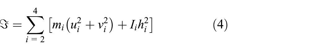
and the centripetal coefficient is determined as

C = \frac{1}{2} \frac{d ℑ}{dq} = \sum_{i = 2}^{4} [m_{i} (u_{i} u_{i}' + v_{i} v_{i}') + I_{i} h_{i} h_{i}']

(5)

where m_i and I_i are the mass and the mass moment of inertia of the link i, respectively; u_i and v_i are the x and y components of the velocity influence coefficients for the mass centre of the link i in Cartesian coordinate system; $u'_{i}$ and $v'_{i}$ define the components of acceleration influence coefficient which are the derivatives of the velocity coefficient with respect to the independent variable q; and h_i and $h'_{i}$ are the velocity and acceleration coefficients corresponding to the rotation of the link i, respectively. The equivalent force can be determined from the virtual power principle $(\overset{\cdot}{W} = Q \overset{\cdot}{q})$ as follows

Q = \sum_{j = 1}^{m} [F_{j}^{x} u_{Fj} + F_{j}^{y} v_{Fj}] + \sum_{i = 2}^{4} T_{i} h_{i}

(6)

where $F_{i}^{x}$ and $F_{i}^{y}$ (j=1,2,…,m) are the components of external or active force; u_Fj and v_Fj are the x and y components of the velocity influence coefficients of the point at which the external force F_j acts. In this study, the external forces F_j are not included and the input torque acting on the crank T₂ is the active force only, so the generalized force is Q = T₂. It should be noted that the nonconservative and dissipative forces can be included in equation (6) when they are presented. The necessary velocity and acceleration influence coefficients of the four-bar mechanism are calculated and given in Appendix 1.

Equations (1) and (3) represent the mathematical model of the DC motor–gearbox mechanism system. For the solution of this equation set, the fourth-order Runge–Kutta method is employed in this study. For this, the new state variables x₁, x₂ and x₃ are introduced as

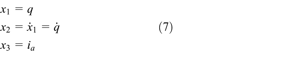
\begin{matrix} x_{1} = q \\ x_{2} = {\overset{\cdot}{x}}_{1} = \overset{\cdot}{q} \\ x_{3} = i_{a} \end{matrix}

(7)

and then the state space equations can be written as

\begin{matrix} {\overset{\cdot}{x}}_{1} = x_{2} \\ {\overset{\cdot}{x}}_{2} = \frac{1}{ℑ + n^{2} J} [- {Cx}_{2}^{2} - n^{2} B x_{2} + n K_{m} x_{3} - n T_{f}] \\ {\overset{\cdot}{x}}_{3} = \frac{1}{L} (V_{a} - R_{a} x_{3} - n K_{g} x_{2}) \end{matrix}

(8)

SMC design

SMC is known as a variable structural control method robustly controlling complex high-order nonlinear systems. The most important advantage of SMC is the insensitivity to parametric variations and external disturbances. In SMC, the user chooses a sliding surface in the state space and the control law forces the state variables to get close to the sliding surface and to slide towards the origin. For a second-order system, there is a sliding surface defined below

s (x, t) = c e_{1} (t) + e_{2} (t)

(9)

where c is a strictly positive real constant which determines the slope of the sliding surface and e₁ and e₂ are the tracking errors defined in the state space as

e (t) = [\begin{matrix} e_{1} (t) & e_{2} (t) \end{matrix}] = [\begin{matrix} x_{1} (t) - x_{d 1} (t) & x_{2} (t) - x_{d 2} (t) \end{matrix}]

(10)

where x_d is the desired trajectory. Equation (9) is a linear homogeneous differential equation for s = 0. In this condition, c is the pole of this equation and the error reaches asymptotically zero for the positive value of c for any initial condition provided that there exists a control law. In order to obtain a control law, a Lyapunov function, which is defined as V(s) = 1/2s² with V(0) = 0 and V(s) > 0 for s > 0, can be used. Consequently, the stability in the sliding mode condition is guaranteed and a good tracking performance can be achieved for $dV / dt = s \overset{\cdot}{s} \leq 0$ .

The general control rule can be chosen as

u (t) = - Ksign (s)

(11)

where u(t) is the control input and K is a strictly positive real constant with a lower bound depending on the estimated system parameters. Note that, in this study, the control input is the motor voltage, V_a, and in the simulations a voltage limit is used to avoid damage to the motor. The control input with the sign function is the discontinuous control law that requires infinite switching on the sliding surface. In this way, the trajectory is forced to always move towards the sliding surface. The switching control signal has an important disadvantage of SMC which is known as chattering. To eliminate chattering, the sign function can be changed by saturation function which can be defined as

sat (s) = {\begin{matrix} s > ε \\ s < - ε \\ - ε < s < ε \end{matrix} \begin{matrix} 1 \\ - 1 \\ s / ε \end{matrix}}

(12)

where ε is a constant which introduces a boundary layer around the switching surface.

MSMC design

In conventional SMC, the sliding surface is fixed with a constant slope of nonoptimal or optimal value of c in the error state space. Hence, if the representative point lies in the stable zone, that is, the second and fourth quadrants in the phase plane, then the absolute value of e₂(t) becomes small for a fixed gain of K when large values are chosen for c. This yields a longer reaching time to the surface s(t). On the other hand, if a small value for c is chosen, the convergence speed on the surface itself will be slow, leading to a longer tracking time. Therefore, if an appropriate small value for a time-varying slope c is chosen, fast tracking will be achieved without increasing the gain K. This is the key feature of the MSS proposed in Choi and Park.¹⁸ The surface is initially chosen to pass arbitrary initial conditions, and the surface is subsequently moved towards the predetermined sliding surface. When the reaching phase is achieved, the movement is terminated and the sliding phase continues with a constant slope value as the conventional SMC. The movement can be executed by rotating/shifting the slope c as shown in Figure 2. Rotating is proposed in the stable zone, while shifting is proposed in the unstable zone. In this article, MSMC with the rotating type of sliding surface is adopted for velocity control of the four-bar linkage. An MSS is proposed such that its time-varying slope is defined as follows

c (t) = c_{0} - (\frac{e_{2} (t)}{e_{1} (t)}); 0 < t < t_{r}

(13)

where c₀ is a positive constant and t_r is the time where the reaching phase is completed. Essentially, the error ratio $e_{2} (t) / e_{1} (t)$ in the equation corresponds to the slope of a surface which satisfies s(t) = 0 at any time t. By adding c₀, a neighbour of this surface is taken to eliminate nonidealities, such as delays. In this way, the surface approaches the representative point and the reaching time is shortened. On the other hand, if the sign of the ratio is negative this means that the error is decreasing and vice versa. However, as the velocity error approaches zero, the magnitude of the ratio and consequently the slope of the surface grow.

Figure 2.

Illustration of moving sliding surface: (a) rotating sliding surface and (b) shifting sliding surface.

It should be noted that, when the mechanism starts to run at zero velocity and acceleration, the velocity error has a negative sign and the acceleration error is zero. Hence, c₀ with a positive value guarantees that the sliding surface is in the stable zone. c₀ is the minimum or the initial value of the slope in this case. On the other hand, at the beginning of the reaching phase, the velocity error decreases, while the acceleration error increases to compensate for the velocity error at first. Then the acceleration error decreases as the velocity error approaches zero. Consequently, the slope changes from a minimum value c_min to a maximum value c_max which are determined by the error ratio at the initial time t₀ and at the final time of the reaching phase t_r, respectively. After the reaching phase is achieved, the movement of the slope is terminated and fixed at its last value. After that, because the sliding phase starts a large positive constant value of c, the velocity error will approach zero asymptotically.

Numerical simulations

For the numerical simulation, a four-bar mechanism and a DC motor without gearbox is considered. The parameters of the motor-mechanism system shown in Figure 1 are given in Table 1.^4,9 The state space representation of the four-bar mechanism and the motor system is simulated using the Runge–Kutta method. A MATLAB code is implemented for the integration of equations of motion given in equation (8). The system is simulated for a 5-s duration with 5 × 10⁻⁴ s time step where the motor voltage is 30 V. The crank angular position and velocity are set to ‘0’ (zero) for the initial conditions. The time history of the crank velocity $(ω_{2} = \overset{\cdot}{q})$ for 2 s is plotted in Figure 3. It is seen that the velocity of the crank fluctuates between 34.903 and 39.465 rad/s after a high level of overshoot.

Table 1.

Mechanism and motor parameters for numerical simulation.^4,9

Mechanism parameters
	Links (i)
		1		2	3	4
r_i (m)		0.5593		0.102	0.610	0.406
c_i (m)				0.0	0.305	0.203
m_i (kg)				1.362	1.362	0.2041
J_i (kg m²)				0.00071	0.0173	0.00509
β_i (rad)				0.0	0.0	0.0
DC motor parameters
R (Ω)	L (H)	K_m (N m/A)	K_g (V s)	J (kg m²)	T_f (N m)	B (N m s)
0.4	0.050	0.678	0.678	0.056	0.00	0.226

V s: Volt-second; N m s: Newton-meter-second.

Figure 3.

Crank velocity for the without-control case.

It is desired that the crank rotates with 30 rad/s constant velocity. To achieve this, both SMC and MSMC methods were applied and the results were compared. The errors e₁ and e₂ are calculated by subtracting the velocity and acceleration values from their desired values at each time step. For the conventional SMC, the parameter c is chosen as 80 which was taken from Şevkat and Telli.⁹ It should be noted that, although the conventional SMC with a filter is used in Kao et al.⁷ and Şevkat and Telli,⁹ it is strengthened with the saturation function to eliminate chattering in this study.

The block diagram of the system with MSMC is shown in Figure 4. For the MSMC, the errors were calculated first, then the specific c values were calculated for each error state satisfying s(t) = 0 by means of equation (13), where c₀ = 6 and t_r = 0.0293. The value of t_r was taken to be slightly smaller than the rise time of the conventional SMC. In this example, the rise time for conventional SMC was found to be 0.0303 s. The control voltage was calculated using equation (11) where the saturation function given in equation (12) was used instead of the sign function. The obtained results, such as average speed, rise time, overshoot and speed fluctuations, for both SMC and MSMC are given in Table 2. The comparison of the crank velocity for MSMC and the conventional SMC with two zoomed regions including the reaching and sliding phases is shown in Figure 5. It is seen that the desired velocity is achieved in a short time in the case of MSMC compared to the conventional SMC, as expected. The rise time for MSMC was determined as 0.0269 s and it is 11.5% shorter than that of the conventional SMC. For the MSMC, the change of the slope and the error ratio with time are shown in Figure 6(a) and (b). It is seen that, while the error ratio is decreasing, the slope increases with time. The slope has a constant value of 100.5 after t_r = 0.0293 s because the moving algorithm was terminated at this time. The discontinuous point on the error ratio graph shows that the representative point crosses the desired velocity, that is, the velocity error is zero. It should be pointed out that because these discontinuities occur after the reaching phase this method is not affected. The time t_r has a crucial role in the performance of the method. The smaller the value of t_r, the longer the reaching time. On the other hand, the larger value of t_r may result in a longer tracking time. The sliding surface for the MSMC is also shown in Figure 7.

Figure 4.

Moving sliding-mode-controlled motor-mechanism system.

Table 2.

Comparison of the velocity parameters for SMC and MSMC.

Control law	Slope c	Average speed	Rise time (s)	Overshoot (%)	Speed fluctuations (%)
No control	–	37.0353	0.1015	57.3415	15.21
SMC	80	30.0047	0.0336	0.1246	0.22
MSMC	Moving	30.0014	0.0269	0.1019	0.19

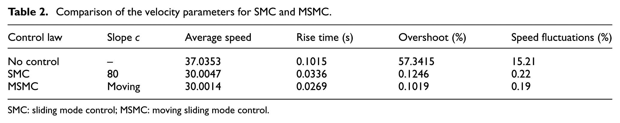
SMC: sliding mode control; MSMC: moving sliding mode control.

Figure 5.

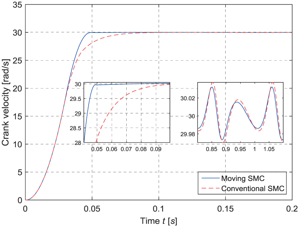
Comparison of the crank velocities for MSMC and conventional SMC.

Figure 6.

Change of (a) slope and (b) error ratio with time, for c₀ = 7 and t_r = 0.0293 s.

Figure 7.

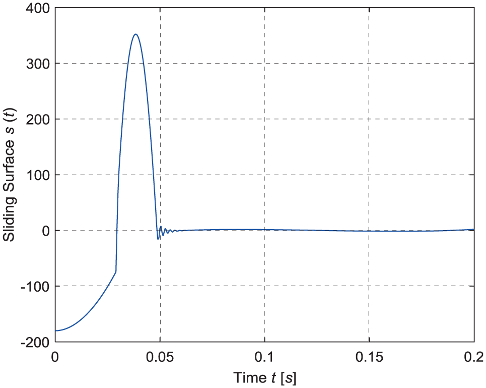
The sliding surface for MSMC.

Experimental study

An experimental system depicted in Figure 8 was set up in order to examine the effectiveness of the control methods. The crank of the four-bar mechanism is driven by a DC motor without gearbox. The parameters of the mechanism and the DC motor are given in Table 3.

Figure 8.

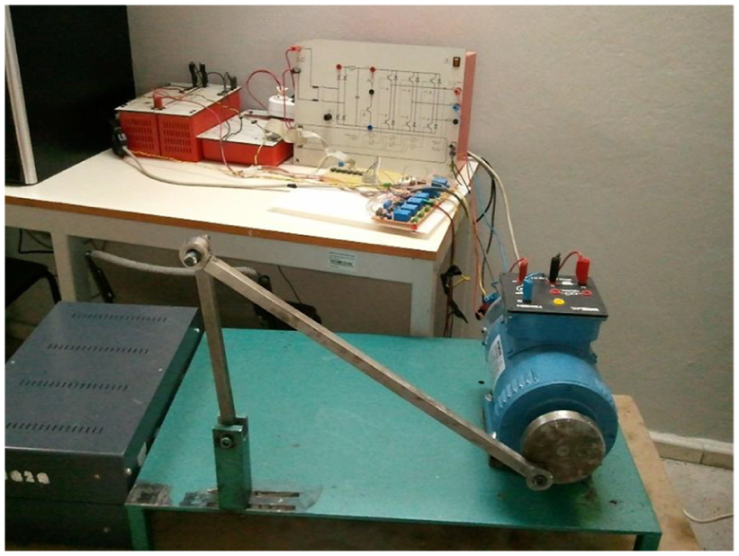
Experimental setup of a four-bar mechanism driven by a DC motor.

Table 3.

Mechanism and motor parameters for the experimental study.

Mechanism parameters
	Links (i)
		1		2	3	4
r_i (m)		0.455		0.045	0.536	0.272
c_i (m)				0.0	0.268	0.136
m_i (kg)				1.311	0.506	0.208
J_i (kg m²)				0.0019	0.0167	0.0058
β_i (rad)				0.0	0.0	0.0
DC motor parameters
R (Ω)	L (H)	K_m (N m/A)	K_g (V)	J (kg m²)	T_f (N m)	B (N m)
25.5871	1.4643	1.0672	1.3758	0.00051	0.00	0.00169
Power (kW)	Torque (N m)	Speed (r/min)	Voltage (V)	Current (A)
1.1	3.2	1500	200	5.5

For the data acquisition and motor control, a dSPACE DS1104 R&D real-time controller board was used. It is fully programmable from the MATLAB/Simulink block diagram environment and all I/O can be configured graphically. After the configuration, the real-time model code can be generated, compiled and automatically downloaded to the DS1104. To drive the motor, an IGBT-based H bridge power convertor was used (Leybold Didactic GmbH, 732 297). The control signal was compared with the ramp function and sent to the DS1104SL_DSP_PWM unit to generate PWM signals for the IGBTs. The angular position and velocity of the crank were measured by a Nemicon NOC-S type 2500 pulse/rev incremental encoder. The block diagram of the real-time control system is depicted in Figure 9.

Figure 9.

Block diagram of the real-time control system.

First, the system was run without any control by applying a constant input voltage of 30 V to the motor. The experiment was performed for 5 s with a time increment of 0.0002 s. Figure 10 shows the step response of the crank angular velocity such that it fluctuates between 13 and 19 rad/s because of the variable inertia.

Figure 10.

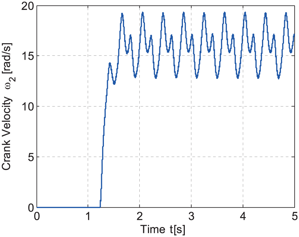
Crank angular velocity for the without-control case in the experimental study.

Second, the conventional SMC was used to control the velocity of the crank. The desired velocity value of the crank was chosen as 20 rad/s. The system was run and the velocity error was determined by comparing the desired velocity and the velocity data taken from the encoder. The motor control voltage was calculated using the velocity error and its derivative in SMC formulas. The PWM signal was generated by the dSPACE DS1104 controller board and applied to the motor driver. The crank velocity is shown in Figure 11(a). Unfortunately, in this case, the desired velocity could not be reached, although it is expected in SMC that the velocity error approaches zero asymptotically in a finite time. It is thought that this unexpected behaviour may be due to the motor trigger rate being lower than the sample time of the applied voltage. It is expected in the SMC that the applied voltage changes between the positive and negative peak values. However, as can be seen in Figure 11(b), the peak voltage value was not reached with few exceptions during the runtime. For this reason, the motor could not reach the desired velocity. In order to avoid damage to the motor, the experiments were not continued for the different SMC parameters.

Figure 11.

(a) Crank velocity and (b) control voltage for the conventional SMC.

Then the proposed MSMC algorithm was applied to control the system and it was observed that the result was very satisfactory. It is evident from Figure 12(a) that the velocity reaches the desired value in a very short time. The crank velocity comes to a stable zone in 0.165 s. The rise time is 0.017 s and the velocity fluctuation is vitally reduced such that the velocity fluctuates between 19.50 and 20.45 rad/s despite the overshoot of 17%. Moreover, the chattering is significantly eliminated as shown in Figure 12(b). These show the efficiency of the proposed MSMC method.

Figure 12.

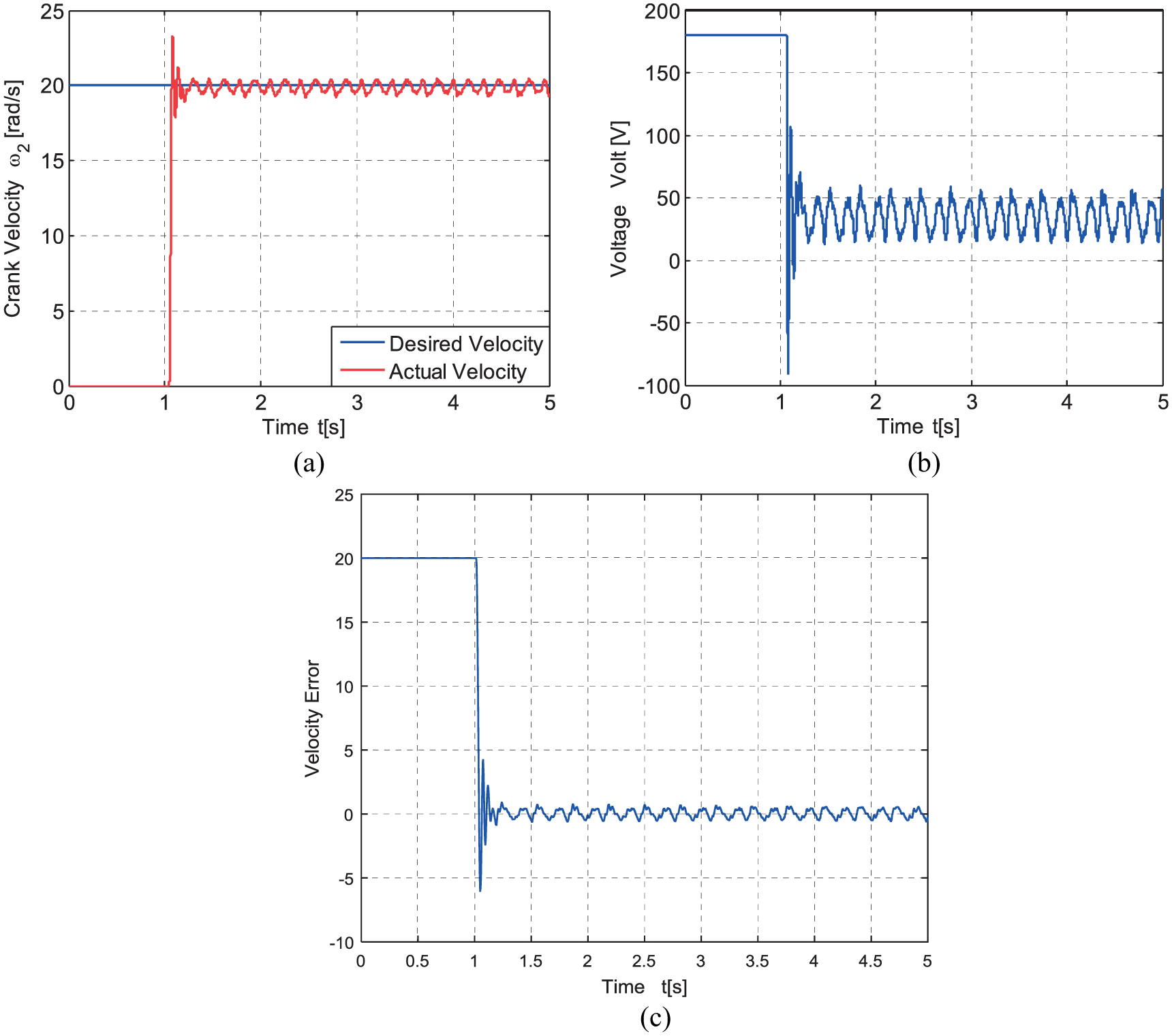
(a) Crank velocity, (b) control voltage and (c) velocity error for MSMC.

One of the important properties of SMC is that it is insensitive to the change of parameters and to the disturbing effects. In order to show the effectiveness of the MSMC over these effects, two experiments were also carried out. In the first case, a 0.5 kg mass is added to link 4 to simulate the change of parameters without changing the controller parameters used in previous experiment. The velocity and voltage responses of the system are shown in Figure 13. It is clearly seen that the method is insensitive to parametric variation.

Figure 13.

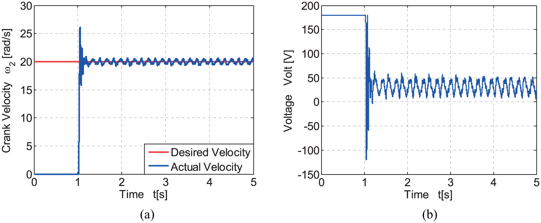
(a) Crank velocity and (b) control voltage in the case of added mass of 0.5 kg.

In the second case, a nonlinear unknown force was simulated by touching to the link 4 suddenly when the mechanism was working. In this case, the amplitude of the force and the time duration were not known. The velocity response and the control voltage are shown in Figure 14. It is seen that the system response is distorted as soon as the force is applied, then the controller stabilizes the crank velocity in about 0.4 s by a large change in control voltage. Note that the experiments were also made for different crank velocities. Similar results were found although the results were not given here for brevity.

Figure 14.

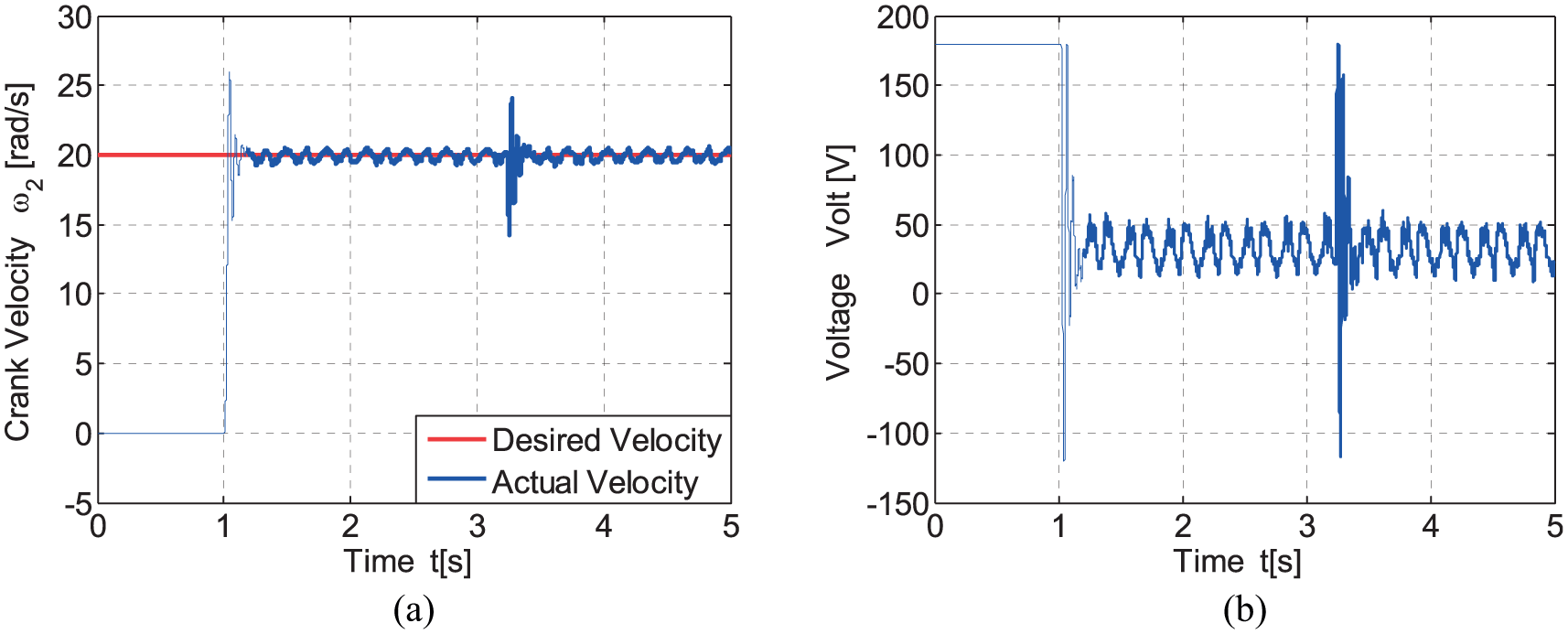
(a) Crank velocity and (b) control voltage in the case of unknown force.

Conclusion

In this study, MSMC was adopted for velocity control of a four-bar mechanism driven by a DC motor. Although, in SMC, the slope of the sliding surface is chosen by the user optimally or nonoptimally, it is calculated based on the error state at each integration of time during the reaching phase in the proposed MSMC. The initial values of the slope and the rotating time have a crucial role in the performance of the proposed method. The rise time of the conventional SMC can be chosen as the time of the rotating procedure terminated.

The numerical simulations as well as the experimental studies showed that the MSMC has a smaller reaching time and robust control compared to the conventional SMC. A most important result observed in the experimental study is that, in the SMC, the desired crank velocity was not achieved. It was thought that this may be because the motor trigger rate is lower than the sample time of the applied voltage. On the contrary, in the case of MSMC, the desired velocity was achieved in a short time that shows the efficiency of the MSMC method.

Footnotes

Appendix 1

The vector loop closure equation of the four-bar linkage shown in Figure 1 can be written as

(14)

A_{0} A + AB = A_{0} B_{0} + B_{0} B

This yields two explicit constraint equations as follows

(15)

\begin{matrix} f_{1} (q, ϕ_{1}, ϕ_{2}) = r_{2} \cos q + r_{3} \cos ϕ_{1} - r_{1} \cos β_{1} - r_{4} \cos ϕ_{2} = 0 \\ f_{2} (q, ϕ_{1}, ϕ_{2}) = r_{2} \sin q + r_{3} \sin ϕ_{1} - r_{1} \sin β_{1} - r_{4} \sin ϕ_{2} = 0 \end{matrix}

The constraint equations are nonlinear and can be solved by the numerical methods for unknown parameters ϕ₁ and ϕ₂.

The velocity coefficient g can be calculated as

(16)

g = - J^{- 1} f'

where

(17)

g = {\begin{matrix} g_{1} & g_{2} \end{matrix}}^{T}, f^{'} = {\begin{matrix} \frac{\partial f_{1}}{\partial q} & \frac{\partial f_{2}}{\partial q} \end{matrix}}^{T}

and J is the Jacobian matrix and the elements of which are given by

(18)

J_{ij} = \frac{\partial f_{i}}{\partial ϕ_{j}}, (i, j = 1, 2)

For the four-bar linkage

(19)

J = [\begin{matrix} - r_{3} \sin ϕ_{1} & r_{4} \sin ϕ_{2} \\ r_{3} \cos ϕ_{1} & - r_{4} \cos ϕ_{2} \end{matrix}], f^{'} = {\begin{matrix} - r_{2} \sin q \\ r_{2} \cos q \end{matrix}}

and the velocity coefficients are determined from equation (16) as follows

(20)

g_{1} = - \frac{r_{2} \sin (q - ϕ_{2})}{r_{3} \sin (ϕ_{1} - ϕ_{2})}, g_{2} = - \frac{r_{2} \sin (q - ϕ_{1})}{r_{4} \sin (ϕ_{1} - ϕ_{2})}

The angular velocity of the links 3 and 4 can be calculated as follows

(21)

{\dot{ϕ}}_{1} = g_{1} \dot{q}, {\dot{ϕ}}_{2} = g_{2} \dot{q}

The velocity of the mass centre of the link i (i = 2, 3, 4), v_Gi, can be calculated as follows

(22)

v_{Gi} = (\sqrt{u_{i}^{2} + v_{i}^{2}}) \overset{\cdot}{q}

where u_i and v_i are the components of the velocity influence coefficient of the mass centre of the link i and they can be determined by differentiating the position variables of the mass centre of the links with respect to the independent variable q

(23)

\begin{matrix} u_{i} = \frac{d x_{i}}{dq} = \frac{\partial x_{i}}{\partial q} + \sum_{j = 1}^{2} \frac{\partial x_{i}}{\partial ϕ_{j}} g_{j} \\ v_{i} = \frac{d y_{i}}{dq} = \frac{\partial y_{i}}{\partial q} + \sum_{j = 1}^{2} \frac{\partial y_{i}}{\partial ϕ_{j}} g_{j} \end{matrix}

For the four-bar mechanism, the coordinates of the mass centre of the links are

(24)

\begin{matrix} x_{2} = c_{2} \cos (q) & y_{2} = c_{2} \sin (q) \\ x_{3} = r_{2} \cos (q) + c_{3} \cos (ϕ_{1}) & y_{3} = r_{2} \sin (q) + c_{3} \sin (ϕ_{1}) \\ x_{4} = c_{4} \cos (ϕ_{2}) & y_{4} = c_{4} \sin (ϕ_{2}) \end{matrix}

and the velocity influence coefficients of the mass centre of the links are determined as follows

(25)

\begin{matrix} u_{2} = - c_{2} \sin (q) & v_{2} = c_{2} \cos (q) \\ u_{3} = - r_{2} \sin (q) - c_{3} \sin (ϕ_{1}) g_{1} & v_{3} = r_{2} \cos (q) + c_{3} \cos (ϕ_{1}) g_{1} \\ u_{4} = - c_{4} \sin (ϕ_{2}) g_{2} & v_{4} = c_{4} \cos (ϕ_{2}) g_{2} \end{matrix}

The acceleration influence coefficient or the second-order influence coefficient is the derivative of the velocity influence coefficient with respect to the independent variable q, and it can be written as

(26)

{g^{'}}_{i} = \frac{d g_{i}}{d q} = \frac{d^{2} ϕ_{i}}{d q^{2}} = \frac{\partial g_{i}}{\partial q} + \sum_{j = 1}^{2} \frac{\partial g_{i}}{\partial ϕ_{j}} g_{j}; i = 1, 2

The acceleration influence coefficients of the four-bar linkage are determined as follows

(27)

\begin{array}{l} {g^{'}}_{1} = - \frac{r_{2} \cos (q - ϕ_{2})}{r_{3} \sin (ϕ_{1} - ϕ_{2})} + \frac{r_{2} \cos (ϕ_{1} - ϕ_{2}) \sin (q - ϕ_{2})}{r_{3} \sin^{2} (ϕ_{1} - ϕ_{2})} g_{1} \\ + \frac{r_{2} \sin (ϕ_{1} - q)}{r_{3} \sin^{2} (ϕ_{1} - ϕ_{2})} g_{2} \end{array}

(28)

\begin{array}{l} {g^{'}}_{2} = - \frac{r_{2} \cos (q - ϕ_{1})}{r_{4} \sin (ϕ_{1} - ϕ_{2})} + \frac{r_{2} \sin (q - ϕ_{2})}{r_{4} \sin^{2} (ϕ_{1} - ϕ_{2})} g_{1} \\ - \frac{r_{2} \cos (ϕ_{1} - ϕ_{2}) \sin (q - ϕ_{1})}{r_{4} \sin^{2} (ϕ_{1} - ϕ_{2})} g_{2} \end{array}

The angular acceleration of the links 3 and 4 can be calculated as follows

(29)

{\overset{\cdot\cdot}{ϕ}}_{1} = g'_{1} {\overset{\cdot}{q}}^{2} + g_{1} \overset{\cdot\cdot}{q}, {\overset{\cdot\cdot}{ϕ}}_{2} = g'_{2} {\overset{\cdot}{q}}^{2} + g_{2} \overset{\cdot\cdot}{q}

The acceleration of the mass centre of the link i (i = 2, 3, 4), a_Gi, can be calculated as follows

(30)

a_{Gi} = (\sqrt{u_{i}'^{2} + v_{i}'^{2}}) {\overset{\cdot}{q}}^{2} + (\sqrt{u_{i}^{2} + v_{i}^{2}}) \overset{\cdot\cdot}{q}

where u_i and v_i are the components of the acceleration influence coefficient of the mass centre of the link i and they can be determined by differentiating the velocity influence coefficient of the mass centre of the links with respect to the independent variable q

(31)

u'_{i} = \frac{\partial u_{i}}{\partial q} + \sum_{j = 1}^{2} \frac{\partial u_{i}}{\partial ϕ_{j}} g_{j}; v'_{i} = \frac{\partial v_{i}}{\partial q} + \sum_{j = 1}^{2} \frac{\partial v_{i}}{\partial ϕ_{j}} g_{j}

For the four-bar mechanism, they are obtained as follows

(32)

\begin{matrix} u_{2}' = - c_{2} \cos (q) \\ v_{2}' = - c_{2} \sin (q) \\ u_{3}' = - r_{2} \cos (q) - c_{3} \cos (ϕ_{1}) g_{1}^{2} - c_{3} \sin (ϕ_{1}) g_{1}' \\ v_{3}' = - r_{2} \sin (q) - c_{3} \sin (ϕ_{1}) g_{1}^{2} + c_{3} \cos (ϕ_{1}) g_{1}' \\ u_{4}' = - c_{4} \cos (ϕ_{2}) g_{2}^{2} - c_{4} \sin (ϕ_{2}) g_{2}' \\ v_{4}' = - c_{4} \sin (ϕ_{2}) g_{2}^{2} + c_{4} \cos (ϕ_{2}) g_{2}' \end{matrix}

Note that in equations (4–6) h_i and $h'_{i}$ are the velocity and acceleration influence coefficients related to the rotation of the links, respectively. For the four-bar mechanism, h_i and $h'_{i} (i = 2, 3, 4)$ are defined as follows

(33)

\begin{matrix} h_{2} = 1, h'_{2} = 1 \\ h_{3} = g_{1}, h'_{3} = g'_{1} \\ h_{4} = g_{2}, h'_{4} = g'_{2} \end{matrix}

From equation (4), the equivalent mass moment of inertia for the four-bar mechanism can be written as

(34)

\begin{matrix} ℑ = m_{2} c_{2}^{2} + I_{2} + m_{3} (r_{2}^{2} + c_{3}^{2} g_{1}^{2} + 2 r_{2} c_{3} \cos (q - ϕ_{1})) \\ + I_{3} g_{1}^{2} + m_{4} c_{4}^{2} g_{2}^{2} + I_{4} g_{2}^{2} \end{matrix}

and its derivative with respect to q divided by 2 which is named as the centripetal coefficient can be found as follows

(35)

\begin{matrix} \frac{1}{2} \frac{d ℑ}{dq} = m_{3} r_{2} c_{3} (g_{1} - 1) \sin (q - ϕ_{1}) + (m_{3} c_{3}^{2} + I_{3}) g_{1} g_{1}' \\ + (m_{4} c_{4}^{2} + I_{4}) g_{2} g_{2}' \end{matrix}

Handling Editor: Yong Chen

Declaration of conflicting interests

The author(s) declared no potential conflicts of interest with respect to the research, authorship and/or publication of this article.

Funding

The author(s) disclosed receipt of the following financial support for the research, authorship, and/or publication of this article: This study was supported by Scientific Research Projects Coordination Unit of Firat University. Project number: FÜBAP-1987.

ORCID iD

Orhan Çakar

References

Sadler

Mayne

Fan

. Generalized study of crank-rocker mechanisms driven by a d.c. motor part I. Mathematical model. Mech Mach Theory 1980; 15: 435–445.

Sadler

Mayne

Fan

. Generalized study of crank-rocker mechanisms driven by a d.c. motor part II. Applications. Mech Mach Theory 1980; 15: 447–461.

Liou

Erdman

Fan

. Dynamic analysis of a motor-gear-mechanism system. Mech Mach Theory 1991; 26: 2399–2252.

Tao

Sadler

. Constant speed control of a motor driven mechanism system. Mech Mach Theory 1995; 30: 737–748.

Lin

Fung

Lin

. Adaptive control of slider-crank mechanism motion: simulations and experiments. Int J Syst Sci 1997; 28: 1227–1238.

Wai

Lin

. A fuzzy neural network controller with adaptive learning rates for nonlinear slider-crank mechanism. Neurocomputing 1998; 20: 295–320.

Kao

Chuang

Fung

. The self-tuning PID control in a slider–crank mechanism system by applying particle swarm optimization approach. Mechatronics 2006; 16: 513–522.

Gündoğdu

Erentürk

. Fuzzy control of a dc motor driven four-bar mechanism. Mechatronics 2005; 15: 423–438.

Şevkat

Telli

. Sliding mode speed control of an electric motor driven four-bar linkage mechanism. Uludağ Universitesi Mühendislik-mimarlık Dergisi 2008; 13: 15–26 (in Turkish).

10.

Fung

Chen

Yen

. Fuzzy sliding mode controlled mechanism using PM synchronous servo motor drive. Int J Mech Sci 1999; 41: 337–355.

11.

Fung

Shaw

. Region-wise linear fuzzy sliding mode control of the motor-mechanism system. J Sound Vib 2000; 234: 471–489.

12.

Lin

Fung

Lin

et al . A supervisory fuzzy neural network controller for slider-crank mechanism. Mechatronics 2001; 11: 227–250.

13.

Lin

Wai

. Sliding-mode-controlled slider-crank mechanism with fuzzy neural network. IEEE T Ind Electron 2001; 48: 60–70.

14.

Hwang

Kuo

. A stable adaptive fuzzy sliding-mode control for affine nonlinear systems with application to four-bar linkage systems. IEEE T Fuzzy Syst 2001; 9: 238–252.

15.

Hwang

Hsieh

. A neuro-adaptive variable structure control for partially unknown nonlinear dynamic systems and its application. IEEE T Contr Syst T 2002; 10: 263–271.

16.

Koca

Akpolat

Özdemir

. Type-2 fuzzy sliding mode control of a four-bar mechanism. Int J Model Simul 2011; 31: 60–68.

17.

Al-Jarrah

Salah

Banihani

et al . Applications of various control schemes on a four-bar linkage mechanism driven by a geared DC motor. WSEAS Trans Syst Contr 2015; 10: 584–597.

18.

Choi

Park

. Moving sliding surface for fast tracking control of second-order dynamic systems. J Dyn Syst: T ASME 1994; 116: 154–158.

19.

Choi

Park

Jayasuriya

. A time-varying sliding surface for fast tracking control of second-order dynamic systems. Automatica 1994; 30: 894–904.

20.

Rye

Durrant-Whyte

. Fuzzy moving sliding mode control with application to robotic manipulators. Automatica 1999; 34: 607–616.

21.

Chun

Sunwoo

. Wheel slip tracking using moving sliding surface. Proc IMechE, Part D: J Automobile Engineering 2005; 219: 31–41.

22.

Alli

Yakut

. Application of robust fuzzy sliding-mode controller with fuzzy moving sliding surfaces for earthquake-excited structures. Struct Eng Mech 2007; 26: 517–544.

23.

Sung

Han

Cho

. Vibration control of vehicle ER suspension system using fuzzy moving sliding mode controller. J Sound Vib 2008; 311: 1004–1019.

24.

Tokat

Eksin

Güzelkaya

. A new design method for sliding mode controllers using a linear time-varying sliding surface. Proc IMechE, Part I: J Systems and Control Engineering 2002; 216: 455–466.

25.

Tokat

S Eksinİ

Güzelkaya

. New approaches for on-line tuning of the linear sliding surface slope in sliding mode controller. Turk J Electr Eng Co 2003; 11: 45–59.

26.

Saeedi

Beheshti

. Optimal design of rotating sliding surface for sliding mode control. In: Proceedings of the American control conference, St. Louis, MO, 10–12 June 2009, pp.774–777. New York: IEEE.

27.

Sumantri

Uchiyama

Sano

et al . Generalized super-twisting sliding mode control with a nonlinear sliding surface for robust and energy-efficient controller of a quad-rotor helicopter. Proc IMechE, Part C: J Mechanical Engineering Science 2017; 231: 2042–2053.

28.

Tanyıldızı

Çakar

. Moving sliding mode control of a DC motor driven four-bar mechanism. In: Proceedings of the AzCIFToMM international symposium of mechanism and machine science, Izmir, 5–8 October 2010, pp.190–197. New York: Curran Associates.

29.

Paul

. Kinematics and dynamics of planar machinery. Upper Saddle River, NJ: Prentice Hall, 1979.

Application of moving sliding mode control for a DC motor driven four-bar mechanism

Abstract

Keywords

Introduction

Mathematical model of a DC motor–gearbox mechanism system

SMC design

MSMC design

Numerical simulations

Experimental study

Conclusion

Footnotes

Appendix 1

Declaration of conflicting interests

Funding

ORCID iD

References