Commissioning new applications on processing machines: Part II – implementation

Abstract

The subject of this splitted article is the commissioning of a new application that may be part of a processing machine. At the example of the intermittent transport of small sized goods, for example, chocolate bars, ideas for increasing the maximum machine performance are discussed. Therefore, optimal process motion profiles are synthesised with the help of a computer simulation. In the first part of the paper, the modelling of the process was shown. This second part focusses on implementing the simulated motion approaches on an experimental test rig, whereby the new motion approach is compared to the conventional approach. Hence, the increasing of the performance can be proven. Eventually, possibilities for an online process control are observed which are necessary to prevent unstable process conditions.

Introduction

From the economic point of view, usually a maximum performance in processing machines is intended. This maximum is limited by several reasons, for example, the rising product load, which increases with the operating speed and may lead to broken goods. For rising the performance of a processing machine, the consideration of the complex process and machine behaviour for motion planning is necessary.^1–3 Here, the often applied principle of the intermittent transport of pieced goods is representatively considered. The aim of this publication is the validation of potentials for rising the maximum performance using a new speed-dependent motion approach which is realised with a modern servo drive. In Part I ⁴ of the paper, the new motion approach was presented (see Figure 1) which will be realised and validated in this article, Part II.

Figure 1.

Comparison of (a) conventional (transport distance is comb distance) and (b) new (transport distance larger than comb distance) product handling.

The new approach theoretically enables an enhancement of the maximal reachable performance in contrast to the conventional motion approach. Due to the strong operating speed dependencies of the new approach, appropriate motion profiles have to be used. For synthesising such profiles, a model was build and verified. This model was used in an algorithm which allows the calculation of an operating speed–dependent optimised set of motion profiles (see Figure 16 in Troll et al. ⁴ ).

In this article, the process model is validated and hence, the new motion approach is implemented and realised on an experimental rig. Therefore, the model parameters have to be identified with the help of experiments on the real active unit. This finally leads to prove the success of the operating speed–dependent motion profiles. Eventually, possibilities to observe this process for the now higher reachable operating speed by the help of high-speed (HS) cameras and simple photoelectric barriers are presented.

Model validation

After verifying the model in Part I, the model has to be validated now. Therefore, the real process parameters have to be identified. The experimental rig is a five-bar linkage with a motion degree of two (2-DoF, see Figure 2). It is expedient to identify the model parameters at the real active unit. As mentioned in Part I, the main model parameters that have to be set are the coefficients of friction and restitution. Therefore, the same experiments as used in the model verification can now be considered for real experiments. Furthermore, the basic parameters, for example, mass and moment of inertia, have to be determined.

Figure 2.

2-DoF mechanism to realise the intermittent transport of pieced goods.

The coefficient of static friction is determined using the experiment of an inclined plane (see Figure 3). The product is in rest on the slide surface, while the system is lifted slowly till the product starts sliding. At this moment, the corresponding angle ${\alpha }_0$ is measured by a digital goniometer. Hence, the coefficient of static friction ${\mu }_{\mathrm{S}}$ can be calculated to

$${\mu }_{\mathrm{S}}=\tan ({\alpha }_0)=0.18$$

(1)

Figure 3.

Identification of the coefficient of static friction.

To identify the coefficient of dynamic friction, a force sensor is used. When the product slides over the slide surface with a constant relative velocity $v_{\mathrm{rel}}$ , the measured friction force $F_{\mathrm{meas}}$ is the only force the engine has to overcome. Therefore, an experimental setup is used as shown in Figure 4. Thus, it is possible to determine the friction at the real active unit. Because the simulation should work for a range of operating speeds, the experiment is executed for an appropriate amount of relative velocities. Measuring the friction forces for different relative velocities leads to the calculation of the coefficient of dynamic friction ${\mu }_{\mathrm{D}}$ by equation (2), where $g$ is the gravitational acceleration and $m_{\mathrm{product}}$ is the mass of the product

$${\mu }_{\mathrm{D}}(v_{\mathrm{rel}})=\frac{m_{\mathrm{product}}·g}{F_{\mathrm{meas}}(v_{\mathrm{rel}})}$$

(2)

Figure 4.

Experimental setup for measuring the coefficient of dynamic friction.

The results of these experiments are plotted in Figure 5. In addition to that, an approximation in form of a rational function is calculated. Thus, the results can be used within the simulation. It can be seen that the coefficient of dynamic friction does not follow a simple law. Instead, the coefficient rises to a maximum for $v_{\mathrm{rel}}=0.5\mathrm{m}/\mathrm{s}$ and then subsides with the relative velocity. This behaviour is already known and described in Popov ⁵ and Braun and Peyrard. ⁶ Finally, the coefficient of restitution $e_{\mathrm{n}}$ has to be identified, which represents the impact behaviour between product and working tool. During the experiments, the comb hits the resting product with a defined and constant velocity $v_{\mathrm{col}}$ , whereby the product instantly moves with the velocity $v_{\mathrm{product}}$ . With the help of a laser distance sensor, the products position is measured and afterwards numerically differentiated. Hence, it is possible to calculate the coefficient of restitution for the specific collision velocity by equation (3):

$$e_{\mathrm{n}}=\frac{v_{\mathrm{product}}-v_{\mathrm{col}}}{v_{\mathrm{col}}}$$

(3)

Figure 5.

Results of measuring the coefficient of dynamic friction.

The results of these experiments are plotted in Figure 6. In contrast to the models for describing the coefficient of restitution (see Part I ⁴ ), the recorded behaviour differs. Usually, the coefficient of restitution is constant and hence independent (linear model), or it subsides with rising collision velocity (Hertzian model). For the considered active unit, $e_{\mathrm{n}}$ first rises below $v_{\mathrm{col}}=0.5\mathrm{m}/\mathrm{s}$ and then subsides. This may be reasoned by additional effects, for example, the influence of friction or soiling on the slide surface, which have higher leverages for small velocities. Therefore, a nonlinear restitution behaviour is considered which can be modelled with a Hertzian-Spring-Dahspot model. Thus, the parameters of the model introduced in Troll et al. ⁴ are fitted to the experimental results.

Figure 6.

Results of measuring the coefficient of restitution.

Implementation of speed-dependent motion profiles

Using the parametrised process model, optimal motion profiles for the new motion approach can be calculated. A characteristic of these optimal motion profiles is their operating speed dependency. The calculated position of the working tool $s$ and the related velocity $v=\stackrel{·}{s}$ are depending on the normalised time $\tau =t/T$ as well as on the considered operating speed $f$ . Therefore, the question is how these special motion profiles can be implemented on an experimental test rig.

As a starting point, the scaling principle is considered which is applied in mechanical mechanisms, for example, cam follower mechanisms. Thereby the position of the working tool is planned over the normalised time; hence, the planned motion does not change by varying the operating speed. Merely the velocity is scaled linear and the acceleration is scaled quadratically to the targeted operating speed. In Figure 7, this relation is shown for the example of the conventional motion approach (see Figure 1(a)). The working tool executes a rise to dwell motion with a transport distance of 0.06 m. The position setpoint is constant for different operating speeds, while the velocity changes linear. With this principle, only one motion is applied on a real machine which is state of the art for servo drives. Hence, the aim of the presented project is to implement a new principle which allows the realisation of multiple given motions for different operating speeds. Therefore, as few as possible, optimised motions have to be calculated and transferred to the servo drive. Following, two strategies are presented.

Figure 7.

Scaling principle applied in mechanical cam follower mechanisms.

Combined scaling and switching principle

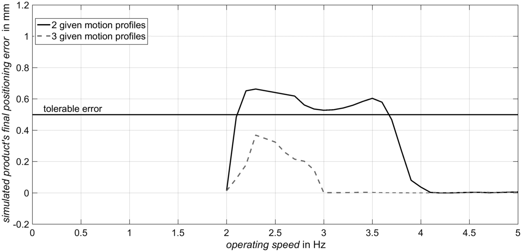
For the implementation of this principle, $n$ optimised motions are assumed for $n$ different operating speeds $f_{\mathrm{opt},1}<f_{\mathrm{opt},2}<\cdots <f_{\mathrm{opt},n}$ . Each optimised motion can be scaled from their rated operating speed to another operating speed. To combine multiple optimised motions, switching speeds $f_{\mathrm{sw}}$ have to be defined which determine the range of validity for every optimised motion. The most simplest possibility for their definition is the determination of the switching speed in the middle of two optimised motions. For a given operating speed, the optimised motion is used whose rated operating speed is closest to the target operating speed. Hence, for $n$ given motion profiles, there are $n-1$ switching operating speeds that are calculated by

$$f_{\mathrm{sw},i}=\frac{f_{\mathrm{opt},i}+f_{\mathrm{opt},i+1}}{2}$$

(4)

whereby $i\in \{1,2,\dots ,n-1\}$ . Defining these switching operating speeds leads to the calculation of the related motions as follows

$$s(f,\tau )=\{\begin{array}{cc}{s}_{\mathrm{opt},1}(\tau ),\hfill & f_{\mathrm{opt},1}\le f\le f_{\mathrm{sw},1}\hfill \\ \multicolumn{1}{c}{}& ⋮\hfill \\ \multicolumn{1}{c}{s_{\mathrm{opt},n}(\tau ),}& f_{\mathrm{sw},n-1}\le f\le f_{\mathrm{opt},n}\hfill \end{array}$$

(5)

as well as the related velocities

$$v(f,\tau )=\{\begin{array}{cc}\frac{f}{f_{\mathrm{opt},1}}·v_{\mathrm{opt},1}(\tau ),\hfill & f_{\mathrm{opt},1}\le f\le f_{\mathrm{sw},1}\hfill \\ \multicolumn{1}{c}{}& ⋮\hfill \\ \multicolumn{1}{c}{\frac{f}{f_{\mathrm{opt},n}}·v_{\mathrm{opt},n}(\tau ),}& f_{\mathrm{sw},n-1}\le f\le f_{\mathrm{opt},n}\hfill \end{array}$$

(6)

In Figure 8, two different implementations of this principle are shown. In the top of the figure, the position and the velocity of two optimised motions for 2 and 5 Hz (black solid lines) are shown. Therefore, one switching speed at $f_{\mathrm{sw},1}=3.5\mathrm{Hz}$ is assumed. It is obvious that there is a discontinuity in the characteristic map because of the speed-dependent optimised motions. In the bottom of the figure, the same principle is applied with three given optimised motions, whereby now two switching speeds are considered. The discontinuities between neighbouring motions are still present, but smaller than assuming only two optimised motions.

Figure 8.

Scaling and switching principle for two (top) and three (bottom) given optimised motion profiles (black lines).

Interpolation principle

Another possibility to combine two or more optimised motions without any discontinuities is the linear interpolation principle introduced in Holowenko et al. ⁷ For implementation, no switching speeds have to be calculated, because the aim of this principle is a continuous trend of the motion profiles. For doing so, first the coefficient $c(f)$ has to be calculated for each targeted operating speed

$$c(f)=\{\begin{array}{cc}\frac{f-f_{\mathrm{opt},1}}{f_{\mathrm{opt},2}-f_{\mathrm{opt},1}},\hfill & f_{\mathrm{opt},1}\le f\le f_{\mathrm{opt},2}\hfill \\ \multicolumn{1}{c}{}& ⋮\hfill \\ \multicolumn{1}{c}{\frac{f-f_{\mathrm{opt},n-1}}{f_{\mathrm{opt},n}-f_{\mathrm{opt},n-1}},}& f_{\mathrm{opt},n-1}\le f\le f_{\mathrm{opt},n}\hfill \end{array}$$

(7)

Second, the position $s(f,\tau )$ over the normalised time $\tau$ can be calculated using equation (8)

$$s(f,\tau )=\{\begin{array}{cc}\frac{s_{\mathrm{opt},1}(\tau )}{\frac{1}{1-c(f)}}+\frac{s_{\mathrm{opt},2}(\tau )}{\frac{1}{c(f)}},\hfill & f_{\mathrm{opt},1}\le f\le f_{\mathrm{opt},2}\hfill \\ \multicolumn{1}{c}{}& ⋮\hfill \\ \multicolumn{1}{c}{\frac{s_{\mathrm{opt},n-1}(\tau )}{\frac{1}{1-c(f)}}+\frac{s_{\mathrm{opt},n}(\tau )}{\frac{1}{c(f)}},}& f_{\mathrm{opt},n-1}\le f\le f_{\mathrm{opt},n}\hfill \end{array}$$

(8)

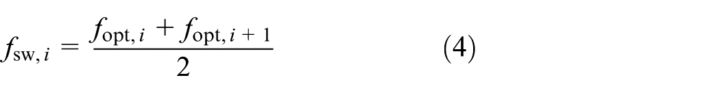
The velocity specifications are calculated analogously. In Figure 9, the results of combining a different amount of optimised motions using the interpolation principle are shown. It can be seen that there are no discontinuities in the characteristic map of the position and velocity, so it is to be expected that using this principle instead of the scaling and switching principle, the process works better for the range of observed operating speeds. This has to be proven by experiments on the test rig which is driven by a motion control system. This allows the specification of a different amount of optimised motion profiles and the combining of these by the two presented principles. Hence, it is possible to compare the advantages and disadvantages of the principles.

Figure 9.

Interpolation principle for two (top) and three (bottom) given optimised motion profiles (black lines).

Increasing the performance using speed-dependent motion profiles

The possibilities of increasing the maximum reachable machine performance using the new motion approach can now be evaluated. First, the conventional motion approach is applied and used as a reference. This allows estimation about the success of the new motion approach. Second, the new motion approach is observed, whereby the two different principles of realising operating speed–dependent motions are used and the related results are discussed. To compare the different approaches and principles, an objective criterion has to be defined. Therefore, the product’s final positioning error is used which is the distance between the intended (in contact with the comb) and the real position of the product at the end of the transport phase. To realise a stable process, an error of less than 0.5 mm is required (tolerable error).

Conventional motion approach

The conventional principle of transporting pieced goods (cf. Figure 1) is applied with a rise to dwell motion of the comb. This motion is planned with a quintic function trajectory and realised with the scaling principle (see Figure 7). The measured results of the product’s final positioning error over the operating speed are plotted in Figure 10.

Figure 10.

Experimental results for the conventional motion approach.

During operating speeds lower than 1.3 Hz, the comb is always in contact with the product and thus, it is positioned exactly. With increasing the operating speed above 1.3 Hz, the positioning error exceeds the tolerable error. Hence, this leads to the maximum reachable performance for this motion approach, because such deviations can induce process instabilities during the return stroke of the working tool. Thus, this motion approach has a principal and physically reasoned border for rising the machine performance.

New motion approach

Now the operating speed–dependent new motion approach is considered, whereby the motion specifications are calculated with the help of the validated process model. Using the new optimised motions, both principles of applying speed-dependent motion profiles are considered, whereby the same optimised motion profiles are used for the different principles. For the sake of simplicity, the optimised motion profiles are calculated for equidistant operating speeds, namely 2, 3.5, and 5 Hz.

In Figure 11, the resulting positioning errors are plotted for the scaling and switching control approach. First, two optimal motion profiles are considered (solid black line). For low operating speeds, the process is quiet inaccurate. The reason for this is that the product’s velocity after detaching the comb’s first tine is not high enough to reach the comb’s second tine. Thus, the positioning error decreases till it attains a minimum at the optimal operating speed of 2 Hz. Scaling this motion profile to higher operating speeds, the positioning error rises again, while it reaches it maximum of 10 mm at a speed of 3 Hz. Increasing the operating speed the error reaches a new minimum for the optimised operating speed of 5 Hz, but the range around the minimum is much wider than it is for the 2 Hz motion.

Figure 11.

Experimental results for different amounts of scaled motion profiles for the new motion approach.

Second, another optimised motion profile for an operating speed of 3.5 Hz is additionally considered. Hence, the maximum positioning error between operating speeds of 2 and 5 Hz decreases from 10 down to 3 mm (see Figure 11, dashed grey graph). Thus, two conclusions can be named because of these experimental results: First, it is proven that the maximum operating speed which leads to a maximum performance can be rised from 1.3 Hz (conventional approach) to 5 Hz by 285% with the help of the new motion approach. Second, the new principle seems to be limited concerning a lower realisable performance. This is reasoned by the required detachment of the product which is compulsory necessary but only occurs for higher operating speeds. Therefore, in the following, the process is only investigated for operating speeds between 2 and 5 Hz.

For implementing this new motion approach on a processing machine, for example, for running up the machine, the final maximum positioning error has to be less than the tolerable error for the named spectrum of targeted operating speeds. As shown in Figure 11, three optimised motion profiles are not enough to fulfil this requirement using the scaling and switching principle. In Holowenko et al., ⁷ using continuous processing with linear interpolation between two motion profiles could lower the positioning error significantly. This will be verified on the presented example.

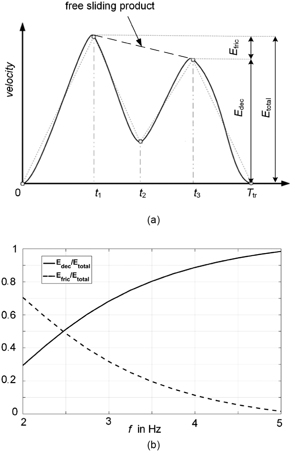
In Figure 12, the product’s final positioning error and the related standard deviations are shown for applying the interpolation principle displayed in Figure 9. Both graphs of the product’s final positioning error show a significant range of maximum values for lower operating speeds, where using two applied optimised motion profiles (solid black line) results in higher positioning errors than three applied optimised motion profiles (dashed grey line). Furthermore, it is obvious that for higher operating speeds, the measured positioning errors are very small, independently from the amount of used optimised motion profiles.

Figure 12.

Experimental results for different amounts of interpolated motion profiles for the motion approach.

On one hand, as expected in Holowenko et al., ⁷ the positioning error could be reduced significantly for two applied motion profiles from 10 to 0.85 mm by 92% only using linear interpolation instead of scaling. Nevertheless, with this result, the maximum position error is still above the tolerable error. Hence, two motion profiles and a linear interpolation in between are not suitable for the new process. For three applied optimised motion profiles, the maximum positioning error could be reduced from 3 to 0.45 mm by 85%. Thus, three optimised motion profiles in association with a linear interpolation are necessary to realise the new motion approach on the given processing machine.

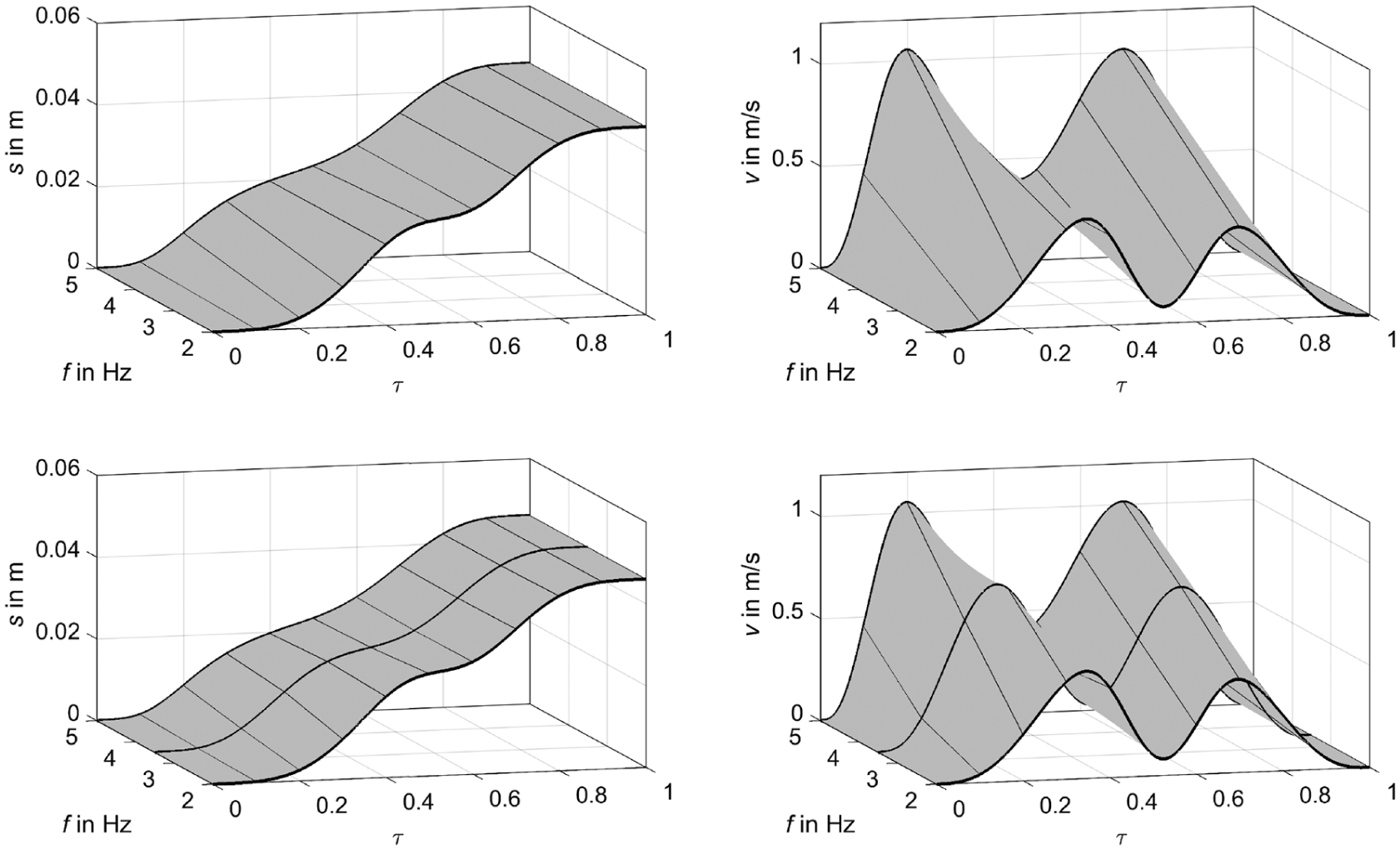
On the other hand, the trends of the experimental results shown in Figure 12 are unexpected regarding the trend of the product’s positioning error. At first sight, a rising of the positioning error with the operating speed would be expected, because of the rising dynamic of the process. Thus, an attempted explanation is presented: the fundament of this explanation is the consideration of the kinetic energy conditions of the product during the transport phase (see Figure 13(a)). The product has a maximum value of velocity at $t_1$ and thus a maximum of kinetic energy of $E_{\mathrm{total}}$ . This energy decreases during the free sliding phase because of the friction by an amount of $E_{\mathrm{fric}}$ . The product’s remaining kinetic energy is converted to the comb’s deceleration energy $E_{\mathrm{dec}}$ . Starting from this observation, the ratios of the friction energy to the total energy and the deceleration energy to the total energy can be plotted for different operating speeds (Figure 13(b)). The amount of friction energy decreases with the operating speed. Hence, the influence of the friction error resulting from the motion profile interpolation subsides with the operating speed. Meanwhile, the comb’s deceleration influence ascends. The more energy of the product is specifically converted to the comb, the more stable the deceleration phase is. Therefore, the product’s final positioning error subsides with the operating speed which has a main influence for rising the maximal machine performance.

Figure 13.

Observation of product’s energy conditions during transport phase.

Another aspect that has to be considered is the non-constant restitution behaviour of the contact. With rising contact velocity, the coefficient of restitution decreases and thus, the influence of the impact to the resulting positioning error subsides. However, it must be said that this relationship has probably less influence than the discussed one of the friction.

Finally, it is examined whether this operating speed–dependent behaviour can also be simulated using the process model. Therefore, the same interpolation principle as well as the same optimised motion profiles used in Figure 12 are applied. The results are shown in Figure 14. Basically, the trends of the graphs are similar to the experimental results. Like in the experimental investigation above, three optimised motion profiles as interpolation base are necessary to undercut the maximum tolerable product’s final positioning error.

Figure 14.

Simulated results for different amounts of interpolated motion profiles for the new motion approach.

However, two differences occur. First, the absolute values of the simulated results are lower than the experimental observed results. Second, the operating speed at which the positioning error decreases for two given motion profiles is higher than experimentally measured. Following, the reasons for these deviations are discussed.

The trend of the decreasing final positioning error for higher operating speeds corresponds with the given energetic explanation. But in difference to the experimental results, the simulated error is exactly zero. This behaviour results out of the fact that the measured model parameters are always related with deviations which are not considered in the simulation, but occur in reality. Thus, small positioning errors can appear during the experiments, because the real parameters of the active unit vary in a small range, whereby the optimised motion profiles are calculated for specific values of the parameters. This may also be the reason for the overall lower values of the positioning errors in comparison to the experimental results. Another difference that stands out is the operating speed at which the graph of the two given motion profiles subsides. This may be reasoned by the incompleteness of the used contact model which was only fitted to the measured coefficient of restitution which is also related with deviations in reality but not in the model.

Despite the discussed deficiencies of the model, the simulation results show a good accordance regarding the main effects of the process behaviour. It can be said that the process model accuracy is sufficient to calculate optimal motion profiles for different operating speeds. In addition to that both the experimental and the simulated results concerning the product’s final positioning errors coincide about the necessary amount of given motion profiles. Thus, a provably higher maximal performance can be realised with this new motion approach in association with a modern servo control. Because of the parameter deviations, small positioning errors may occur during the process. Therefore, some possibilities for an expedient online process control are presented.

Online process control

If the process is not parametrised well or the starting position of the product is not as accurate as required, the product may be placed incorrectly after the transport phase. This effect is illustrated in Figure 15. In this figure, the product positions in the stable case are marked with dashed lines. The first column shows the end of the transport phase and hence the starting position of the return stroke. In case of the stable process, in this position, both tines are in contact with the product. As can be seen in ①, the rear tine is not in contact to the product. Columns B to E show the beginning of the return stroke where in the stable case the comb is not touching the product. In the shown instable case, the left rear tine touches the product in ②, followed by an unexpected product motion (D, E). If in this situation the comb’s return stroke would be finished in the regular way, the comb and the product would collide. To avoid this situation, a collision avoidance system is needed which not only monitors the comb’s, but also the product’s motion.

Figure 15.

Instable process resulting from wrong product positioning (1) and unexpected product–gripper–contact (2).

The main functionality of the collision avoidance system is to check whether the product reaches a desired position on a given trigger time. Three key requirements are given for the system. First, position and trigger time have to be configurable. Second, the measurement has to be without contact to the product to avoid instability of the process. Finally, the measurement has to be real time capable to ensure a fast enough reaction in case of a pending collision.

The allowed reaction time in case of a collision depends on the desired operating speed and the parameterisation of the stopping ramp. In any case, the comb needs to be stopped within its return stroke before touching the product. Considering 5 Hz as a maximum operating speed, one cycle of the comb is done within 200 ms and the return stroke takes about 120 ms. If the comb should stop from full speed, a maximum stopping time has to be defined. The assumption that the emergency stopping profile is faster than a regular motion profile leads to a maximum allowed stopping time of 60 ms. The reaction time of the control system has to be less than the remaining 60 ms, so following a limit of 30 ms is intended.

Different sensor types are available which fulfil the requirements of a contactless measurement, for example, laser-, ultrasonic- or inductive-working sensors or imaging techniques. Following some examples are discussed concerning their versatility for the considered problem.

As an example of imaging techniques HS cameras are discussed. The use of such techniques is well known in processing machines.^8,9 On one hand, these systems are flexible in use for different types of measurements, so they are often used in analysing processing machines. On the other hand, HS cameras are very expensive compared to other types of sensors and for getting satisfying results, the operator has to consider multiple requirements of the system. Using a HS camera system is suitable if an existing machine has to be commissioned to a new process without adding sensors. While measuring a process, a camera has to be located next to the process, looking at the product from a save position. The required product position can be investigated by analysing the pictures in special evaluation software.^10,11

Camera measurement assembly used for demonstration in this work is illustrated in Figure 16. The machine control introduced in Großmann et al.^12,13 is connected via EtherCAT to an image processing system, consisting of a HS camera and an evaluation software. The function of the collision detection software is the execution of a command like ‘test for collision on position X’, or another query. The required test positions are represented by target positions in the picture (see Figure 16, target). If the distance between the product in the actual picture and the predefined target is too large, a pending collision has been detected; otherwise, no collision should occur. This collision state is returned to the machine control that reacts in case of a forthcoming collision with a fault reaction. The interactions of the machine control and the image processing system have been investigated, especially under the focus of real-time capability. It has been shown that a maximum reaction time of 2.5 ms can be guaranteed. Thus, this type of collision control system fits the requirements. In further works, the implementation of the software could be optimised to lower the reaction time. As mentioned HS cameras provide a big flexibility, but if this is not the main target, other cheaper sensor types can be used. Following, an appropriate alternative is presented.

Figure 16.

Measurement assembly if high-speed camera is used.

Another possibility to apply an online process control is the use of stationary and firmly installed sensors, for example, photoelectric barriers. In this case, four sensors are installed to observe four products which are transported at the same time (see Figure 17). With the help of the sensor, the control can check whether a product is at the expected position at a specific time. The signal evaluation takes place with the control frequency of 8 kHz. Thus, a misplaced product is detected after a time of 0.125 ms. If such a signal is detected, an emergency stop is induced, so a collision of the comb with the product is prevented. Hence, similar results as with a HS camera can be achieved.

Figure 17.

Measurement assembly if photoelectric barrier is used.

In contrast to the HS camera, the photoelectric sensors are much cheaper, have a higher reliability, and are easy to maintain. The main disadvantage in using photoelectric sensors is the fact that only the product monitoring time is programmable (first key requirement). If the product’s dimensions change, the sensors have to be adjusted again which is associated with additional non-production time.

Summary

In this splitted paper, a new method for increasing the maximum performance of a processing machine was discussed. At the example of the intermittent transport of pieced goods, it has been shown that by changing the motion approach, the performance can be rised significantly. For realising this, a process model has been build and verified, described in Part I of the paper. It was shown that with the help of the process model, motion profiles could be calculated for the new motion approach. In Part II, the process model was validated at the real active unit so a computer simulation of the process became possible. The novelty of the new motion approach is the operating speed dependency. That means that for each targeted operating speed, another motion profile is optimal for the process. Different optimised motion profiles were calculated for different operating speeds using the validated process model.

The success of these optimised motion profiles were tested on an experimental test rig. As a reference, the conventional motion approach was also applied, whereby the maximum reachable performance was determined for an operating speed of 1.3 Hz. In the next step, two different principles for combining multiple optimised motion profiles with the servo control were tested. Hence, the maximum reachable performance was determined for an operating speed of 5 Hz, whereby the performance of the machine was increased by 285%. These results were also evaluated by simulations with the process model. Eventually, different opportunities for realising an online control were shown to monitor and evaluate the process. This helps to prevent unstable conditions of the process but also leads to possibilities for the online adapting of the motion profiles. This could be necessary if the process parameters change during execution. In future works, the investigations presented here are transferred to other process classes applied in processing machines, including the implementation of the optimised motion profiles.