Sage Journals: Discover world-class research

Abstract

A core-driven fan stage operates in both single bypass and double bypass modes. There are large differences in aerodynamic parameters between the two modes. To accommodate the differences, the inlet guide vanes must turn in a very large angle, which may cause significant flow losses. To reduce the flow losses, this article investigates three design schemes in detail using the flow field simulation method. The three schemes investigated include the inlet guide vanes adjusting entirely (Scheme 1), the rear part of the inlet guide vanes adjusting (Scheme 2), and both the front and rear part of the inlet guide vanes adjusting (Scheme 3). Comparisons of the three design schemes suggest that the flow losses in Scheme 1 are higher than those in the other two schemes and that the flow losses in Scheme 3 are not evidently lower than those in Scheme 2. The key geometrical parameters of Schemes 1 and 2 are determined for low flow losses and are used to design the inlet guide vanes. The inlet guide vanes are applied to a core-driven fan stage, and the flow fields are simulated by a three-dimensional flow simulation method to confirm the designs.

Keywords

Inlet guide vane core-driven fan stage variable guide vane aeroengine flow field simulation

Introduction

Variable-cycle engines (VCEs) can vary their bypass ratio to create a high bypass ratio for low take-off noise and high subsonic cruise economical efficiency or a low bypass ratio for high thrust during supersonic cruising.^1,2 The core-driven fan stage (CDFS) is a key component in a VCE. The CDFS concept was first proposed by GE and applied to the VCE technology demonstrator known as YJ101, which was tested between 1978 and 1981.^3–5 Afterward, the CDFS was used in a VCE known as GE21 designed by GE.^6,7 The fourth-generation engine YF120 is a typical representative of VCEs.⁸

To consider the different requirements of air mass flow and pressure ratio in the two operational modes, the inlet guide vanes (IGVs) of the CDFS are usually designed to be geometrically adjustable. When the single bypass (SB) mode is switched to the double bypass (DB) mode, the IGV turning angles are large as approximately 30°, which increases difficulties of the IGV aerodynamic design.⁹ Variable camber guide vanes (VIGVs) are applied to prevent large flow losses from large flow attack angles. VIGVs are split into the front and rear parts. The front parts are fixed, while the rear parts are rotatable.^3,10 VIGVs are also used widely in fans of conventional turbo-engines for adjusting their working lines.^11,12 M Boehle et al.¹³ compared the flow fields of VIGVs with that of invariable inlet guide vanes (IIGVs) and determined that the VIGVs had a favorable pressure distribution on the vane surfaces in comparison with the IIGVs and that the flow losses of the VIGVs were lower than those of the IIGVs. C Celis et al.¹⁴ proposed correction factors that can be used to modify the compressor characteristics map as a function of the VIGV angles.

This article presented comparisons of three schemes of the IGVs in a CDFS, which are the IGVs adjusting entirely, the rear part of the IGVs adjusting, and both the front and rear part of the IGVs adjusting. From detailed flow analysis, influences of key geometrical parameters to flows in the IGVs were revealed, and characteristics of the three schemes were exhibited. The obtained results could assist to engine designers in selection of the IGV scheme and its design, to minimize the origin of dangerous flow losses and separation. Large flow separation areas on IGV profiles surfaces occur at high attack angles. In some unfavorable conditions, flow vortexes can be shed off in the flow directions. This phenomenon can cause high intensive blade vibrations in the case of resonance. It is often connected with blades failure.

Three design schemes of IGVs

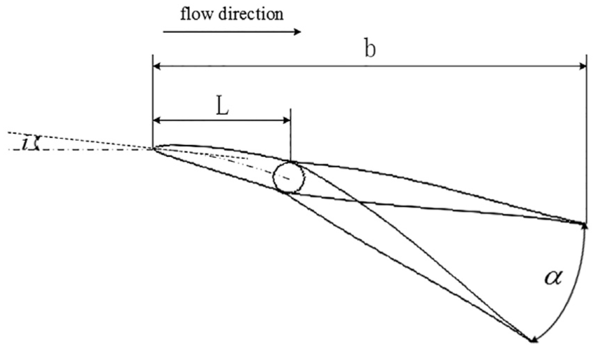
In this article, IGV aerodynamic design schemes were investigated to reduce the original IGV flow losses for a designed CDFS, and three schemes were investigated. The first, referred to as Scheme 1, consists of the IGV entirely adjusting, in which the IGV can be rotated around its rotating axis, as shown in Figure 1. The second, referred to as Scheme 2, consists of the front and rear part of the IGV, in which the front part is fixed and the rear part can be rotated around the axis, as shown in Figure 2. The third, referred to as Scheme 3, consists of also the front and rear parts of the IGV, in which the front and rear blade parts can both be turned around the axis, as also shown in Figure 2.

Figure 1.

IGV entirely adjusting scheme.

Figure 2.

IGV camber variable schemes.

Among the three schemes, Scheme 1 is the simplest in structure, and Scheme 3 is the most complex. If the flow attack angle in one mode of Scheme 1 is small, the attack angle in the other mode must be large. For example, if the attack angle in the SB mode is 0°, it will become a large positive value in the DB mode, which may cause large flow losses. The small attack angles in the two modes of Schemes 2 and 3 can be maintained, but the rear part must be turned by a large degree in one mode, which may cause large flow losses. The flow losses and flow characteristics of the three schemes are compared in the following sections.

Analyses of the three schemes

The IGV scheme research in this article aims to improve the existing design, which means that the distributions of outlet flow angles along the vane spans in the two modes are known. Because the outlet flow angles in the two modes vary gently along the span, there are no large differences between the flow fields at every vane span. Only profiles at 50% vane span were selected for investigation of the three schemes. Table 1 shows the inlet and outlet boundary conditions at the design point.

Table 1.

Inlet and outlet boundary conditions at 50% blade span.

	SB mode	DB mode
Inlet flow angle (°)	0	0
Outlet flow angle (°)	8.62	36.77
Inlet total temperature (K)	288.15	288.15
Inlet total pressure (Pa)	101,325	101,325
Outlet static pressure (Pa)	82,850.7	85,402.6
Inlet flow Mach number	0.524	0.372
Inlet flow Reynolds number	547,522	393,357

SB: single bypass; DB: double bypass.

IGV entirely adjusting scheme (Scheme 1)

From Table 1, due to a flow turning angle of only 8.62° in the SB mode, the IGV camber (θ) is small (approximately 10°) when the camber is determined according to the flow turning angle in the SB mode. In this case, the flow consists of a large positive attack angle in the DB mode, causing an increase in the boundary layer thicknesses on the blade suction surfaces despite the flow passages being generally convergent, as shown in Figure 3(a). However, if the camber is determined according to the flow turning angle (36.77° from Table 1) in the DB mode, the camber will be quite large (approximately 40°). In this case, the flow consists of a large negative attack angle in the SB mode, causing an increase in the boundary layer thicknesses on the blade pressure surfaces, as shown in Figure 3(b). Thus, considering the two modes, the IGV camber should fall between the above two values, and it is necessary to search for the optimal value. In the following search, the variation range of the camber was set from 10° to 40°.

Figure 3.

Mach number contours of two extreme cambers in Scheme 1: (a) θ = 18° and (b) θ = 30°.

To investigate the influences of the IGV camber on the flow losses in the two modes, four blade profiles with cambers of 18°, 22°, 26°, and 30° were generated using the standard NACA65 blade model. First, the four cascade solidities were all taken as 1.5.

For simulating flow fields in the cascades, the two-dimensional (2D) Reynolds-averaged Navier–Stokes equations (including mass, momentum, and energy conservation equations) were used and discretized by the central spatial discretization scheme; and the Spalart–Allmaras (SA) turbulence model was selected for the equation closure. The grid number was approximately 15,000, and the grid was inspected quantitatively, which includes orthogonality, aspect ratio, and extension ratio; in addition, most y⁺ values on the wall were within 3.

The flow attack angles in the four cascades were adjusted repeatedly to ensure their outlet flow angles in the two modes (8.62° in the SB mode and 36.77° in the DB mode). The calculation results in Table 2 show that the differences between the designated outlet flow angles and actual values in most cases were smaller than 1.0°. As shown in Table 2 and Figure 4, in the SB mode, with an increase in the camber, the negative attack angle increases, which causes an increase in the total pressure loss coefficient. However, in the DB mode, with an increase in the camber, the positive attack angle decreases, which causes a decrease in the total pressure loss coefficient. Thus, the total pressure loss coefficient decreases first and then increases with an increase in the camber. Large negative attack angle or large positive attack angle would cause flow separation. Thus, there is a blade camber corresponding to the minimum total flow losses, which is approximately 26°, and the sum of total pressure loss coefficient is 0.0906, as seen in Table 2 and Figure 4. The total pressure loss coefficient ζ in this article is defined by formula (1), in which $P_{1}^{*}$ and $P_{2}^{*}$ are inlet and outlet total pressure while $P_{1}$ is inlet static pressure

ζ = \frac{P_{1}^{*} - P_{2}^{*}}{P_{1}^{*} - P_{1}}

(1)

Table 2.

Calculation results.

Camber (°)	Operational mode	Outlet flow angle (°)	Total pressure loss coefficient	Attack angle (°)	Sum of total pressure loss coefficient
18	SB	8.21	0.0243	−9	0.1394
18	DB	36.23	0.1151	19	0.1394
22	SB	8.02	0.0278	−13	0.1049
22	DB	35.94	0.0771	15	0.1049
26	SB	7.83	0.0362	−17	0.0906
26	DB	35.76	0.0545	11	0.0906
30	SB	7.68	0.0534	−21	0.0976
30	DB	35.57	0.0442	7.5	0.0976

SB: single bypass; DB: double bypass.

Figure 4.

Relationship between total pressure loss coefficient and the IGV camber.

To further consider influences of the cascade solidity, the flow fields of the cascades with solidities of 1.0, 1.25, 1.5, and 1.75 and a blade camber of 26° were simulated. The flow deviation angles vary with the cascade solidity and influence the outlet flow angles. The stagger angles of the blades in the cascades were adjusted slightly to ensure the outlet flow angles. From Figure 5, in the SB mode, the flow losses increase with an increase in the solidity. In this mode, the boundary layers on the blade surfaces are thin, and flow losses are low. With an increase in the solidity, the boundary layers occupy more flow space in the cascades, and the flow losses increase. In the DB mode, with an increase in the solidity, the flow losses decrease at first and then increase due to the combining influences of suppression of the boundary layer development and increase in the ratio of the boundary layers to the main flow. There is a solidity (equal to 1.5) corresponding to the minimum flow loss sum of the two modes. From Figure 5, if the cascade solidity is between 1.25 and 1.5, the loss sum is relatively low. From Figure 6, it can be seen that with an increase in the solidity, the boundary layer thickness on the blade suction surfaces in the DB mode obviously decreases. The blade solidity $τ$ defined by formula (2), in which b is blade profile chord length while t is tangential spacing of the profiles

τ = \frac{b}{t}

(2)

Figure 5.

Relationship between total pressure loss and solidity.

Figure 6.

Mach number contours in the cascades with two extreme solidities: (a) solidity equal to 1.0 and (b) solidity equal to 1.75.

IGV camber variable scheme (Schemes 2 and 3)

The IGV camber variable scheme includes two schemes: the IGV rear part adjusting (Scheme 2) and the IGV front part and rear part adjusting (Scheme 3). For Scheme 2, the IGV front part is fixed, and the attack angle (angle i, seen in Figure 2) of the front part is the key parameter affecting the flow losses in both modes. If a small attack angle is set in the SB mode, the flow losses will be low due to the small flow outlet angle and therefore small flow turning angle. However, the flow losses will be high in the DB mode due to the large flow outlet angle and therefore large deflection angle between the front and rear parts. Otherwise, the flow losses may be large in the SB mode because of a large flow attack angle, and the losses may decrease in the DB mode because of the small deflection angle. In addition, the camber of the base blade (original blade) determines the deflection angle between the front and rear part in the two modes and is a key parameter affecting the flow losses.

Four base blades of different cambers were constructed for researching Scheme 2, and the attack angles and deflection angles were adjusted for given outlet flow angles in the two modes. The joint point of the front and rear parts was set at a 30% chord length from the leading edge.¹⁵ There should be clearance between the front and rear parts for their relative motion, but it was neglected in this research. Based on preceding research, the solidities of the cascades composed of these blades were all set to 1.5 at first. In all cases, the differences between the given outlet flow angles and actual flow angles were controlled within values smaller than 1.0°, which were realized by adjusting the rear parts repeatedly.

In Figure 7, for a certain blade camber (θ for the SB mode), an increase in the attack angle (i) resulted in the flow loss increasing due to increases in thicknesses of the boundary layers on the blade suction surfaces (which can be seen from comparison between Figure 8(a) to (b) and (c) to (d)). When the attack angle is 0°, the loss is minimal. It can also be seen in Figure 7 that under a certain attack angle, with an increase in the blade camber (θ), the flow loss increases, and the increase extent rises with an increase in the attack angle. This is also due to the increase in thicknesses of the boundary layers on the blade suction surfaces, which can be seen more clearly from a comparison between Figure 8(b) and (d).

Figure 7.

Total pressure loss coefficient in the SB mode.

Figure 8.

Mach number contours of the IGV camber variable scheme: (a) i = 0°, θ = 9°; (b) i = 14°, θ = 9°; (c) i = 0°, θ = 20°; and (d) i = 14°, θ = 20°.

In Figure 9, for the DB mode under a certain attack angle, the loss changes are quite small with variation of the blade camber, except for the case of the attack angle equal to 0° and the camber equal to 9°. In this case, there is a large deflection at the joint point of the front and rear parts, which causes large local flow variation (seen in Figure 8(a)), and the flow losses are relatively high. For most of the blade cambers, if the attack angle is in the range of 0°–7°, the flow losses are relatively low. However, the losses increase rapidly with an increase in the attack angle when the angle is larger than 7°. Generally, in the DB mode, the cascade passages are convergent, and the flow is in the negative pressure gradient. Thus, the rear part of the blade does not cause large local flow losses. From Figure 8(a) and (c), it can be seen that at the attack angle equal to 0°, the boundary layers on the blade surfaces are thin if the cambers are equal to 9° and 20° for the DB mode. However, at a large attack angle, although corresponding to small blade deflection, the boundary layers on the blade suction surfaces become thick and the blade wakes become large. As can be seen in Figure 8(b) and (d) for the DB mode at the attack angle equal to 14°, the flow losses increase.

Figure 9.

Total pressure loss coefficient in the DB mode.

The sum of the losses in the two modes is shown in Figure 10. In the figure, the sum loss is low when the attack angle is small (smaller than 7°). The loss in the SB and DB modes is low at small attack angles. The deflection of the blade in the DB mode is large, though it did not cause high flow losses. It can also be seen in Figure 10 that at a small attack angle, when the camber is between 9° and 20°, the flow loss remains nearly unchanged with the camber variation. This shows that the sum loss is not sensitive to the base blade camber if the attack angle is small.

Figure 10.

Sum of the total pressure loss coefficient.

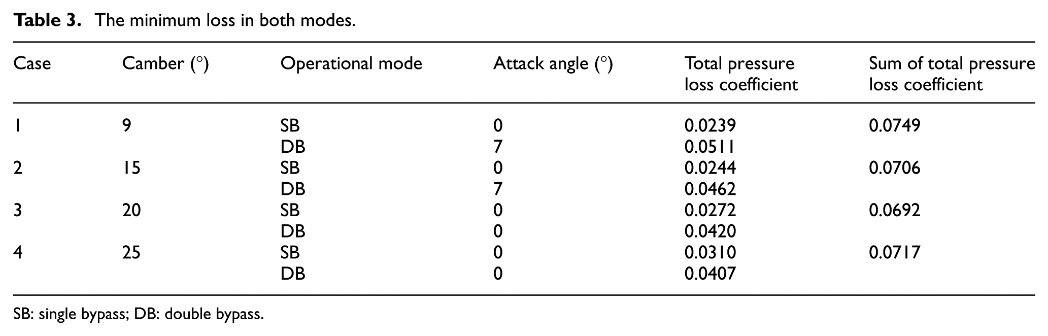
Table 3 lists the attack angles corresponding to the minimum loss in both modes and the sum losses at every camber. In Scheme 3, due to the front part of the IGV being adjustable, the attack angles in the two modes can be set as different values. Thus, in Table 3, the sum of the total pressure loss coefficient at every camber is the minimum of the sum, which Scheme 3 can arrive at but Scheme 2 cannot if the attack angles on the two modes in the table are not equal. Considering the minimum sum losses, case 3 in the table was selected, namely, a camber value equal to 20° and an attack angle equal to 0° in both modes. Thus, the attack angle does not need to be changed from one mode to the other, and the front part does not need to be adjustable. Therefore, Scheme 3 can be replaced by Scheme 2. Figure 10 implies that the total pressure loss coefficient remains nearly unchanged with the variation of the attack angle when the angle is less than 7°.

Table 3.

The minimum loss in both modes.

Case	Camber (°)	Operational mode	Attack angle (°)	Total pressure loss coefficient	Sum of total pressure loss coefficient
1	9	SB	0	0.0239	0.0749
1	9	DB	7	0.0511	0.0749
2	15	SB	0	0.0244	0.0706
2	15	DB	7	0.0462	0.0706
3	20	SB	0	0.0272	0.0692
3	20	DB	0	0.0420	0.0692
4	25	SB	0	0.0310	0.0717
4	25	DB	0	0.0407	0.0717

SB: single bypass; DB: double bypass.

The cascade solidity in the above investigations for Schemes 2 and 3 is 1.5. Figure 11 presents the influences of the solidity on the flow losses in the two modes. With regard to the sum loss, the solidity should be less than 1.0, but the loss decreases gently with a decrease in the solidity when it is less than 1.25.

Figure 11.

Relationship between total pressure loss coefficient and the solidity.

IGV three-dimensional blade designs and their application

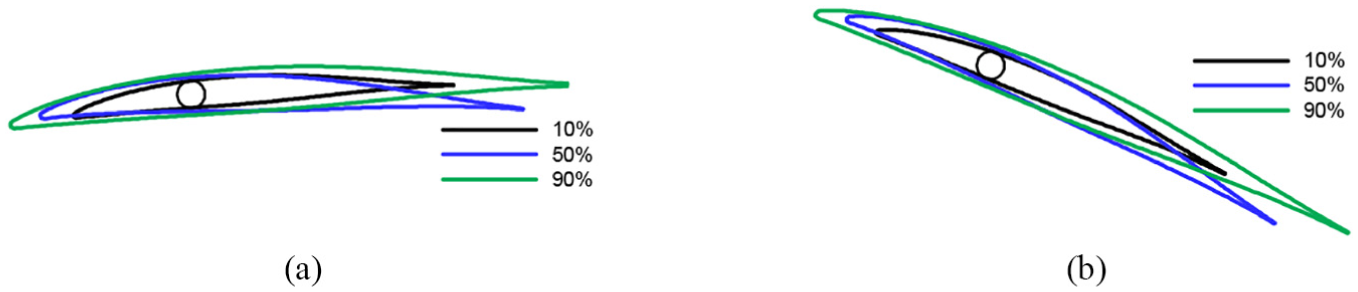
From the analysis of the IGV design schemes at the 50% span, Schemes 1 and 2 were selected for designing the IGV three-dimensional (3D) blades. The key geometrical parameters are listed in Table 4, which are based on the minimum sum losses. The blade profiles at the other span positions were designed based on the same parameters listed in Table 4. The flow outlet angles in the two modes vary along the span, as seen in Figure 12. Thus, the profile stagger angle in Scheme 1 and the rear part deflection angle in Scheme 2 vary along the span. Figures 13 and 14 give the profiles at the 10%, 50%, and 90% spans.

Table 4.

Key geometrical parameters in the two modes.

	Camber (°)	Solidity	Attack angle (°)
Scheme 1	26	1.5	–
Scheme 2	20	1.0	0

Figure 12.

Distribution of IGV outlet flow angles along the span in two modes.

Figure 13.

Blade profiles in Scheme 1: (a) SB mode and (b) DB mode.

Figure 14.

Blade profiles in Scheme 2: (a) SB mode and (b) DB mode.

The original IGVs in the CDFS were replaced by the IGVs designed above. The 3D flow fields of the CDFS with the newly designed IGVs were simulated by the NUMECA software. The 3D Reynolds-averaged Navier–Stokes equations were used and discretized by the central spatial discretization scheme; and the SA turbulence model was selected for the equation closure. Conservative coupling by pitchwise row was adopted for the rotor–stator interfaces. The rotor tip clearance was 0.5 mm. The numbers of grid nodes of the IGV, rotor, and stator were 0.35, 0.52, and 0.32 million, respectively, to insure that y⁺ at all walls was smaller than 10.

From Table 5, the total pressure recovery coefficients of the IGVs designed by the two schemes are quite high in the two modes. In the two modes, the total pressure recovery coefficients of the IGV designed by Scheme 2 are higher than those of the IGV designed by Scheme 1. The efficiencies of the CDFS with the IGV designed by Scheme 2 are higher than those of the IGV designed by Scheme 1. However, the differences in the total pressure recovery coefficients and the efficiencies between the two schemes are small, and the differences in the CDFS performance lines, seen in Figure 15, are also small. Thus, Scheme 1 can also be selected for its simple structure.

Table 5.

Design indices and 3D calculation results.

		IGV total pressure recovery coefficient	Efficiency	Total pressure ratio	Relative flow mass
SB mode	Design index	–	0.8700	1.654	1.000
	Scheme 1	0.9946	0.8653	1.693	0.999
	Scheme 2	0.9960	0.8730	1.657	1.001
DB mode	Design index	–	0.8650	1.369	0.751
	Scheme 1	0.9946	0.8658	1.367	0.758
	Scheme 2	0.9959	0.8729	1.368	0.762

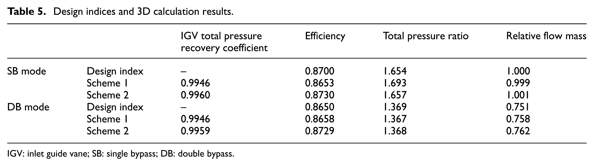
IGV: inlet guide vane; SB: single bypass; DB: double bypass.

Figure 15.

Characteristic lines of the CDFS: (a) total pressure ratio and (b) efficiency.

Conclusion

This article investigated in detail three IGV schemes using a flow field simulation method. From the analysis of the influences of the base blade camber and attack angle on the flow losses, it was concluded that the flow losses in Scheme 3 were not evidently lower than those in Scheme 2 and that the flow losses in Scheme 1 were larger than those in the other two schemes.

The key geometrical parameters of Schemes 1 and 2 resulting in low flow losses were determined and used to design the IGVs, which were applied to a CDFS. The flow field simulation results show that the efficiency of the CDFS with the IGV designed by Scheme 2 was lower than that of the CDFS with the IGV designed by Scheme 1, though the difference was not large. Thus, Scheme 1 can also be selected for its simple structure.

Footnotes

Appendix 1

Handling Editor: Assunta Andreozzi

Declaration of conflicting interests

The author(s) declared no potential conflicts of interest with respect to the research, authorship, and/or publication of this article.

Funding

The author(s) received no financial support for the research, authorship, and/or publication of this article.

References

Fishbach

Stitt

Stone

et al . NASA research in supersonic propulsion: a decade of progress. In: 18th joint propulsion conference, Cleveland, OH, 21–23 June 1982. Reston, VA: AIAA.

Rallabhandi

Mavris

DN.

Simultaneous airframe and propulsion cycle optimization for supersonic aircraft design. J Aircraft 2008; 45: 38–55.

French

Allen

NASA VCE test bed engine aerodynamic performance characteristics and test results. In: 17th joint propulsion conference, Colorado Springs, CO, 27–29 July 1981. Reston, VA: AIAA.

Vdoviak

Knott

Ebacker

JA.

Aerodynamic/acoustic performance of Yj101/double bypass VCE with coannular plug nozzle. Patent NASA-CR-159869, USA, 1981.

Vdoviak

Ebacker

JA.

VCE test bed engine for supersonic cruise research, 1979, pp.347–356, https://ntrs.nasa.gov/search.jsp?R=19810009472

Morris

Coen

Geiselhart

KA.

Performance potential of an advanced technology Mach 3 turbojet engine installed on a conceptual high-speed civil transport. Technical Report, NASA Langley Research Center, Hampton, VA, November 1989.

Krebs

Allan

RD.

Supersonic propulsion—1970 to 1977. In: 13th joint propulsion conference, Orlando, FL, 11–13 July 1977. Reston, VA: AIAA.

AIAA-2006-7976. Research on TBCC propulsion for a Ma 4.5 supersonic cruise airliner.

Lai

AQ.

Research on aerodynamic design of core driven fan stage. Master’s Thesis, Nanjing University of Aeronautics and Astronautics, Nanjing, China, 2013, pp.35–59 (in Chinese).

10.

Mcdow

RW.

Variable inlet guide vane. Patent 4856962, USA, 1989.

11.

Bobula

Soder

Burkarolt

. Effect of a part-span variable inlet guide vane on the performance of a high-bypass turbofan engine. In: 17th joint propulsion conference, Colorado Springs, CO, 27–29 July 1981. Reston, VA: AIAA.

12.

Woollett

. Aerodynamic performance of a fan stage utilizing variable inlet guide vanes for thrust modulation. In: 19th joint propulsion conference, Seattle, WA, 27–29 June 1983. Reston, VA: AIAA.

13.

Boehle

Cagna

Itter

Compressible flow in inlet guide vanes with mechanical flaps. In: ASME turbo expo 2004: power for land, sea, and air, Vienna, 14–17 June 2004, pp.341–349. New York: ASME.

14.

Celis

Pinto

PDMR

Barbosa

et al . Modeling of variable inlet guide vanes affects on a one shaft industrial gas turbine used in a combined cycle application. In: ASME turbo expo 2008: power for land, sea, and air, Berlin, 9–13 June 2008. New York: ASME.

15.

Lai

BF.

Scheme on aerodynamic design of core driven fan stage. J Aerosp Power 2014; 29: 2229–2238 (in Chinese).

Aerodynamic design schemes of the inlet guide vane in a core-driven fan stage

Abstract

Keywords

Introduction

Three design schemes of IGVs

Analyses of the three schemes

IGV entirely adjusting scheme (Scheme 1)

IGV camber variable scheme (Schemes 2 and 3)

IGV three-dimensional blade designs and their application

Conclusion

Footnotes

Appendix 1

Declaration of conflicting interests

Funding

References