Sage Journals: Discover world-class research

Abstract

A wind tower can augment the performance of a vertical-axis wind turbine since it can increase the wind velocity as well as adjust the wind direction. However, it is very important to correctly determine the configuration of the wind tower because the wind tower can also interrupt the wind flow toward the wind turbine. Hence, a numerical analysis was conducted to investigate an effective wind tower configuration using computational fluid dynamics. For practical reasons, a numerical algorithm using a reduced computational domain was applied because the full three-dimensional computational fluid dynamics required huge amounts of computation time for a transient analysis. This method was validated using experimental results and was then applied to the computation of a wind tower with an installed vertical-axis wind turbine. Three wind tower design parameters were chosen for investigation: the inner radius, outer radius, and relative angle of the guide wall. When these parameters were correctly determined, the wind tower always increased the performance of the vertical-axis wind turbine in an omnidirectional wind. In addition, the maximum power coefficient was increased from 0.261 (without the wind tower) to 0.436.

Keywords

Vertical-axis wind turbine wind tower guide walls computational fluid dynamics performance augment

Introduction

Global demand for renewable energy will continue to increase due to the steady depletion of fossil fuels. Efforts to develop sources of energy to replace fossil fuels are being conducted in various fields, including solar, geothermal, ocean, waste heat, and wind power. To exploit wind power, wind energy is converted to mechanical energy by a wind turbine, and then, electrical energy is produced by rotating a generator with this mechanical energy. The attainable output power depends on the size of the wind turbines and wind velocity. Wind turbines are typically divided into horizontal-axis wind turbines (HAWT) and vertical-axis wind turbines (VAWTs) based on the rotational direction in relation to the wind direction.

VAWTs are widely used, even in urban settings, because they have several advantages, including low noise, a simple structure which does not need a yaw control device, and easy installation of the generator near the ground. However, their efficiency is degraded because they operate in a complex flow field of spreading trailing vortices which are detached from the preceding blade. The efficiency of a wind turbine greatly depends on how effectively a turbine blade can convert wind energy to mechanical energy. Therefore, considerable research^1–3 has been conducted to develop a better blade which can efficiently convert wind energy at appropriate Reynolds numbers,^4–6 corresponding to the wind velocity. This effort is necessary because many wind turbine airfoils were developed at approximately one-order higher Reynolds number for aircraft wings.

The blades of the VAWT operate vertically in relation to the wind direction. As a result, they do not need a yaw control, but their output power greatly depends on their relative position against the wind direction. This phenomenon is due to the variation in the angle of attack of the blade. If a better angle of attack can be formed, the performance of the wind turbine can be improved. For this purpose, guide vanes^7–9 have been applied to adjust the flow direction and ensure that the blade maintains a better angle of attack. Experimental results¹⁰ have shown that the power coefficient could be improved by 75% when the guide vane was set appropriately.

In order to access higher wind power, wind turbines can be installed at high elevations or at the edge of a building roof.^11,12 If a diffuser is installed at the rear of the wind turbine, it augments the wind turbine’s output power^13–15 by increasing the pressure difference between the fore and aft sections of the wind turbine. The increased pressure difference results in improved wind turbine performance. However, applying a diffuser to a VAWT is not easy because the diffuser needs a yaw control device. To address this issue, diffusers^16,17 are typically installed around vertical wind turbines so that they can work without yaw control.

When diffusers are installed around a VAWT, they act as an omnidirectional guide vane and have improved the wind turbine power by 3.48 times at peak torque.¹⁶ However, the improvement in VAWT performance provided by guide vanes cannot be simply predicted using the single streamtube model or multiple-streamtube model^18,19 which were developed to evaluate the aerodynamic performance of VAWTs. Such prediction requires a computational study for various geometries of the guide vanes in an omnidirectional wind. A two-dimensional (2D) computational investigation was conducted, and the results showed that the power coefficient was increased by around 30%–35% when compared to stand-alone operation.²⁰

A review of previous research efforts to improve the performance of the VAWT reveals many feasible approaches. In this study, the wind tower shown in Figure 1 was adopted because it has several merits, including high elevation, an omnidirectional guide vane, and the installation of many wind turbines in a single tower. The wind tower has the potential to significantly improve the performance of the VAWT without using a yaw control device. However, the wind tower can also degrade the performance of the VAWT depending on its configuration because the wind flow could be blocked by the tower. Therefore, the configuration of the wind tower was investigated to determine the design parameters, so that the VAWT would always achieve best performance in an omnidirectional wind. In addition, a numerical method using a reduced computational domain was investigated as a practical tool to predict the performance of the VAWT installed within a wind tower.

Figure 1.

View of a wind tower with installed VAWTs.

Numerical method

Computed results can differ depending on the size of the computational domain, the number of grid elements, the turbulence model, the first grid near wall, and so on. Hence, for computations involving the VAWT, studies have been conducted to determine an appropriate turbulence model^21–24 because flow structures within the VAWT are complex. These studies showed better prediction results when the shear stress transport (SST) k–ω turbulence model was applied. However, to investigate the performance of the VAWT, the computation requires a transient analysis because the torque on a blade varies depending on its location during rotation.

For a VAWT having three blades, a 2D computation needs approximately 300,000 grids and more than 10 rotations to get a stable result in the transient analysis. This requires computational time of almost 24 h using a PC (4.0 GHz quad-core CPU). Even though the computational time greatly depends on the computational algorithm and the performance of the PC, it nonetheless requires a huge amount of computational time if the analysis is extended to a three-dimensional (3D) domain. For this reason, although some have been computed in three-dimensions,^25,26 many computational studies have been conducted using a 2D domain.^27–29

Depending on the computational domain, the computational algorithms can be classified as 2D, two and a half dimensional (2.5D), or 3D analyses. The 2.5D analysis uses the computational domain of only a part of the blade in the spanwise direction instead of the full blade. The computed result using the 2.5D analysis provided a better result than that using 2D analysis.³⁰ In this study, the 2.5D analysis was adopted as a practical method to investigate the performance of the VAWT, and then, this method was validated using experimental results from the literature.

CFX³¹ was adopted for the numerical analysis, and the computational domain consisted of three domains: the core region, blade region, and outer region as shown in Figure 2. The core and blade regions rotate in the transient analysis, and they slide at the interface with the outer region. Before starting the transient analysis, a fully converged result was obtained for the steady-state. This result was used as an initial state in the transient analysis. For comparison with the experimental results, flow conditions in the experiment were applied to the boundaries of the computational domain. A high-resolution method was used for the discretization of convective terms, and the second-order backward Euler scheme was applied in the transient analysis. The SST model was adopted for turbulence analysis, and this was solved by the high-resolution scheme, which provides better accuracy in boundary layers on unstructured meshes. An automatic scheme was applied to the wall function, and the first grids on the blade were carefully treated so that they were located within the sublayer. In the transient analysis, the rotational angle in a time step was set to 1°, which was more restricted than the time step recommended by CFX. When the rotational angle in a time step was reduced to less than 1°, the difference between the computed results was insignificant.^21,32 The maximum number of iterations per time step was set to 10 and the root-mean-square (RMS) residual target was set to $1.0 \times 10^{- 5}$ . In order to obtain a completely consistent result, the computation was conducted for up to 10 rotations.

Figure 2.

Computational domain and grids (reduced for better view).

Validation of numerical method

Among many experimental results, three experimental results^32–34 were selected so that a numerical validation could be conducted with various solidities of VAWTs. Table 1 shows the specifications of the VAWT and the experimental facility.

Table 1.

Specification of VAWTs and experimental conditions.

	Castelli³²	Howell³³	Takao³⁴
Blade profile	NACA0021	NACA0022	NACA0015
Blade chord, $c$ (mm)	85.8	100	137
Blade radius, $r_{w}$ (mm)	515	300	300
Blade span, $H$ (mm)	1456.4	400	700
Wind velocity, $V_{\infty}$ (m/s)	9	3.16–5.45	9
Number of blade, $N$	3	3	3
Blade solidity, $σ$	0.25	0.5	0.685
Maximum power coefficient, $C_{p}$	0.31	0.18	0.09
Tip speed ratio, $λ_{o p t}$	2.6	2.1	1.1
Wind tunnel height (m)	4.0	1.2	–
Wind tunnel width (m)	4.0	1.2	–
Wind tunnel diameter (m)	–	–	1.8
Blockage	9.38%	16.70%	16.50%

VAWT: vertical-axis wind turbine.

Comparison with Castelli’s results

The VAWT used in the experiment³² had a low solidity character. Since the 2.5D analysis was applied, the height $(Δ l)$ of the computational domain in the spanwise direction was set to the blade chord length. The computed torque in the transient analysis periodically varied depending on the location. Hence, this torque $(Π)$ was averaged based on a period $(T)$ and then compensated by the blade span $(H)$ as shown in equation (1)

Π = \frac{1}{T} \int_{0}^{T} (\frac{H}{Δ l} \int_{0}^{Δ l} d τ) d t

(1)

where $d τ$ in equation (1) includes the force $(f_{p})$ produced by the pressure on a blade and the force $(f_{v})$ produced by viscosity. The forces of the pressure contributed to the rotational torque depending on the directional vector at each grid surface. The total rotational torque including the viscous forces was obtained as in equation (2)

d τ = \sum_{i}^{n} [{\vec{r}}_{i} \times {(f_{p})}_{i}] + \sum_{i}^{n} [{\vec{r}}_{i} \times {(f_{v})}_{i}]

(2)

where $n$ in equation (2) means the number of grids on the blade surface and $r_{i}$ is the radius from the shaft of the wind turbine.

Grid independency was tested at the optimal tip speed ratio of $λ (R ω / V_{\infty}) = 2.52$ , which was determined when the power coefficient was maximized. Figure 3 shows the variation in the power coefficients computed with various numbers of grids and the non-dimensional distances $(y^{+})$ on the blade surface. The power coefficient was gradually converged by increasing the numbers of grids or reducing the maximum distance of the first grid on the blade surface. This means that the change in torque retarded by the viscous force would be insignificant if all first grids $(y^{+})$ are located within the sublayer. Thus, the correct output power was obtained as long as the first grids on the blade were located within the sublayer.

Figure 3.

Variation in power coefficients depending on the grids: (a) number of elements and (b) non-dimensional distance.

Figure 4 shows the power coefficients computed with a coarse grid (grid-B), and a fine grid (grid-G) is shown in Figure 3. As expected, the peak power coefficient was larger than that in the experiment, and also the application of different grids resulted in different power coefficients. The computed optimal tip speed ratio was larger than that in experiment, and the power coefficients in the range of low tip speed ratio were less than those in the experiment. In this computation with two different grids, an interesting point was observed that the optimal tip speed ratio was obtained near the same point even though different power coefficients were obtained. The cause of this phenomenon will be described together with a comparison of other experimental results in section “Discussion of three comparison cases.” In order to compare these results with a 2D computational analysis, the computed results reported by Castelli³² are illustrated in Figure 4.

Figure 4.

Comparison of power coefficients with the experimental and computational results.³²

Comparison with Howell’s results

The VAWT in this experiment had a solidity of 0.5, and it was tested under velocities ranging from 3.16 to 5.45 m/s. In the computation, a velocity of 4.31 m/s was selected to compare with not only the experimental result but also the computed result reported by Howell et al.,³³ who performed a 2D computation. The first grid near the blade was determined to be less than $y^{+} = 2$ . The height of the computation domain in the spanwise direction was set to half of the blade chord. Figure 5 shows the computed power coefficients with the experimental result and the computed result reported by Howell. The computed result showed a trend similar to that discussed in section “Comparison with Castelli’s results,” with a larger optimal tip speed ratio and low-power coefficients in the range of low tip speed ratio. This same trend was shown in the computed result reported by Howell et al.³³

Figure 5.

Comparison of power coefficients with the experimental and computational results.³³

Comparison with Takao’s results

In the experiment conducted by Takao et al.,³⁴ the VAWT had the largest solidity of 0.685. Figure 6 shows the computed results with the experimental results. Three different grids were applied to investigate their effect at the optimal speed ratio. The “grid-K” was a fine grid, but the “grid-M” was a coarse grid, in that its first grids were located in the log-region. For these three different grids, the optimal tip speed ratio for each was obtained near $λ = 1.71$ even though the computed power coefficients were different. These results mean that the variation in the rotational speed affected the performance of the VAWT more significantly than the difference in the grids. In Figure 6, the experimental results reported by Castelli et al.³² and Howell et al.³³ are illustrated to show the difference between each experimental result, even though they cannot be directly compared with each other due to the different experimental conditions.

Figure 6.

Comparison of power coefficients obtained using different grids with the experimental result.³⁴

Discussion of three comparison cases

Table 2 shows the optimal tip speed ratio and the maximum power coefficient obtained using the 2.5D computation, compared with those measured in the three experiments. In addition, it shows the ratio of the computed value to the measured value. Since the 2.5D computation did not consider the loss generated by the arm struts and at the blade tip, it is natural that the computed results would be better than the experimental results. In the 2D computation conducted by Castelli et al.³² and Howell et al.,³³ the maximum power coefficients of 0.56 and 0.37 were obtained, respectively. Thus, the power coefficient ratios became 1.81 and 2.05, respectively; these are greater than 1.35 and 1.67 obtained in the 2.5D computation. Accordingly, it can be considered that the 2.5D computation is more accurate than the 2D computation because a finite computational domain along the spanwise direction was added in the 2.5D computation.

Table 2.

Comparison of the optimal tip speed ratio and the maximum power coefficient.

	$λ_{o p t}$		$C_{p, m a x}$		$λ_{o p t}$ ratio	$C_{p, m a x}$ ratio
	Exp.	Comp.	Exp.	Comp.	(Comp./Exp.)	(Comp./Exp.)
Castelli et al.³²	2.6	3.25	0.31	0.42 (0.56³²)	1.25	1.35 (1.81³²)
Howell et al.³³	2.1	2.28	0.18	0.30 (0.37³³)	1.09	1.67 (2.05³³)
Takao et al.³⁴	1.1	1.71	0.09	0.31	1.55	3.44

The solidity of the VAWT was the largest in Takao et al.’s³⁴ experiment. Hence, it can be predicted that the optimal tip speed ratio will be lower than those measured in the other two experiments.^32,33 This prediction is clearly shown in not only the experimental results but also the computed results. However, the maximum power coefficient ratio shown in Table 2 was larger than those in other two experiments. This resulted from the low-power coefficient in the experiment. In Takao et al.’s³⁴ experiment, the size of the VAWT was bigger than that in Howell et al.’s³³ experiment, and moreover, the wind velocity was twice higher. The low-power coefficient could be caused by the larger solidity. In the computation, the maximum power coefficient computed based on Takao’s VAWT model was slightly larger than that computed with Howell’s model. Therefore, the 2.5D computation provides consistent results according to the experimental conditions. Thus, this computational method was applied to investigate an applicable wind tower configuration.

Comparison between a 2.5D and a 3D computation

In order to compare the 2.5D and the 3D computational results, the VAWT used in Takao et al.’s³⁴ experiment was adopted. Figure 7 shows streamlines, which were obtained using the 2.5D computation, in the center plane of the span. The computed results in the outer region are illustrated based on the stationary frame, but those in the blade and core region are illustrated based on the rotating frame, as shown in Figure 7(a). In addition, Figure 7(b) illustrates streamlines only in the stationary frame at the same blade location. In the 2.5D computation, the difference between the flow structures along the spanwise direction was insignificant because the computation was conducted as if the blade had an infinite length. The flow structure within the VAWT showed a strong vortex located near the azimuth angle of $θ = 180 °$ .

Figure 7.

Streamlines in the center plane of the computational domain in the 2.5D computation: (a) rotating frame and (b) stationary frame.

In the flow structures obtained using the 3D computation, a strong vortex also appeared in the center plane of the span, as shown in Figure 8(a). However, the strength of this vortex was gradually weakened as the plane moved toward the blade tip, as shown in Figure 8(b) and (c). In order to investigate the effect of the vortex within the VAWT, the torque in the blade was determined at the same tip speed ratio along the rotational direction.

Figure 8.

Comparison of streamlines along the spanwise direction in the 3D computation: (a) at the center plane of the span, (b) at the plane of H*0.25 from the span center, and (c) at the plane of H*0.5 (blade tip).

Figure 9 shows the difference in torque coefficients obtained with the 2.5D computation and the 3D computation. In the 2.5D computation, the height of the computational domain was tested with three different lengths, which were 10%, 20%, and 50% of the blade span. The difference in the computed results was insignificant, as shown in Figure 9. Most of the positive torque was obtained in the range of 19° < $θ$ < 113°. However, in the 3D computation, the range was extended to 19° < $θ$ < 170°. Even though the range for generating torque was extended, the periodic average torque was reduced because of the diminished vortex toward the blade tip, as shown in Figure 8. In the 2.5D computation, the vortex within the rotating region increased the positive and negative peak torque. As a result, the periodic average torque was increased compared to the results obtained with the 3D computation. Hence, this caused that the power coefficient predicted by the 2.5D computation could be overestimated.

Figure 9.

Comparison of torque coefficients obtained with various spanwise computational domains and 3D computation at $λ = 0.81$ .

One of the important purposes of this study was to investigate the potential for predicting the performance of a VAWT using a reduced computational domain and a reduced number of grids. While the applied method cannot predict the true performance value of the VAWT, it could be a very useful tool for comparing relative value. For instance, when designing both a wind tower and a VAWT, there are many design variables that should be determined. These design variables can be optimized using an optimization technique, if the adopted numerical method provides consistent results for various operating conditions. Therefore, this 2.5D analysis can be applied to the design of a wind tower.

Wind tower and wind turbine

A wind tower was employed to improve the performance of a VAWT, as shown in Figure 1. VAWTs were installed at the center of the wind tower. Guide walls around the VAWT were installed to support each floor of the wind tower. These guide walls were utilized to not only change wind flow direction but also to provide access to more wind energy. This would allow the VAWT within the wind tower to operate at a better angle of attack as well as receive more wind energy. However, the effect of the guide wall greatly depends on the relative location of the guide wall with respect to the wind direction. Thus, it was necessary to investigate the correct guide wall configuration considering an omnidirectional wind.

Seven guide walls were employed as shown in the cross-sectional view of the wind tower, which is illustrated in Figure 10. The number of guide walls was determined based on an experiment. The experiment showed that a wind tower installing seven guide walls exhibited better VAWT performance than the others. A VAWT installed within the wind tower had five blades, and its solidity $(σ = cN / 2 r_{w})$ was 0.688. For solidity, “c” and “N” mean the chord of the blade and the number of blades, respectively. The NACA0018 profile was used for the blade profile. In order to modify the wind tower configuration, three major design parameters were selected, the inner radius $(r_{i})$ , outer radius $(r_{o})$ , and relative angle $(β)$ , against the wind direction, as shown in Figure 10.

Figure 10.

Geometrical parameters within a wind tower.

If the inner radius $(r_{i})$ of the wind tower is increased without changing the wind turbine, the operation of the VAWT is equivalent to a stand-alone operation. In contrast, if this inner radius is decreased, then the wind velocity can be increased within the wind tower. The highest wind velocity is produced near the edge of the guide wall and the wind direction is also abruptly changed there. Therefore, the performance of the VAWT is greatly affected by the inner radius parameter.

The outer radius $(r_{o})$ of the guide wall determines the size of the wind tower. The performance of the VAWT can be increased if the outer radius is increased, but its effect can be limited. Hence, an appropriate outer radius should be determined that does not result in a loss of performance. The relative angle $(β)$ of the guide wall is also an important parameter because the performance of the VAWT installed within the wind tower should be evaluated in an omnidirectional wind. Except for these three parameters, the thickness of the guide wall, the direction of the guide wall, and so on have an insignificant effect on the performance of the VAWT.

The computational grid, which is reduced for better view, is shown with the VAWT and guide walls in Figure 11. Total pressure was applied to the inlet boundary condition because this condition can be considered a natural phenomenon. In the computation, the applied total pressure was 40 Pa larger than the static pressure. At the exit, a static pressure was applied. The performances of the VAWTs were compared based on a design point operating at a tip speed ratio of $λ = 2.2$ . Its performance was computed using the same algorithm applied in section “Validation of numerical method.”

Figure 11.

Grids in a horizontal plane (reduced for better view).

The relative angle parameter $(β)$

When the wind blows parallel to a guide wall, the relative angle $(β)$ becomes zero, as shown in Figure 10. In the computation, other parameters were fixed, such that the inner radius and outer radius of the guide wall became $r_{i} / r_{w} = 1.5$ and $r_{o} / r_{w} = 3.75$ , respectively. To obtain a reference performance for the VAWT, a computation was conducted on the VAWT alone without the wind tower. Table 3 shows the periodic averaged torque coefficients with various relative angles. When $β = 25.71 °$ , the periodic averaged torque coefficient was worse than that obtained without the wind tower. This means that the wind tower can deteriorate the performance of the VAWT depending on the relative angle.

Table 3.

Periodic averaged torque coefficient with various relative angles of guide wall.

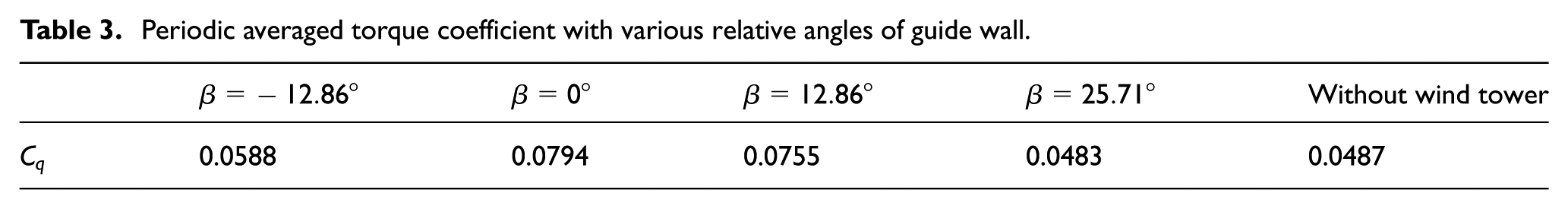
	$β = - 12.86 °$	$β = 0 °$	$β = 12.86 °$	$β = 25.71 °$	Without wind tower
$C_{q}$	0.0588	0.0794	0.0755	0.0483	0.0487

Figure 12 shows the variation in torque coefficient $(C_{q} = Π / (0.5 ρ {AV}_{\infty}^{2} r_{w}))$ obtained at one blade along the rotational direction. The frontal area $(A)$ of the wind turbine was determined using the span $(H)$ of the turbine blade and the rotational diameter $(2 r_{w})$ of the turbine. Most of the output power of the VAWT was obtained in the fore region, which is from 0° to 180° in azimuth angle. However, these torque coefficients had different results for different relative angles. When the relative angle was less, the positive torque started early and decayed early too. In the fore region, the torque decreased and increased again before reaching the maximum torque. This phenomenon occurred due to the rear flow from the guide wall located in the middle of the fore region.

Figure 12.

Variation in the torque coefficients along the rotational direction $(r_{o} / r_{w} = 3.75, ε = 0.5)$ .

The inner radius parameter $(r_{i})$

The output power of the VAWT is affected by the wind flow rate, wind pressure, wind velocity, wind direction, and so on. The inner radius of the guide wall can affect the wind direction and velocity on the rotating blades of the VAWT. For a fixed blade rotating radius $(r_{w})$ , the inner radius was non-dimensionalized as a gap $(ε = (r_{i} - r_{w}) / r_{w})$ . The performance of the VAWT was computed with various gaps, but the other parameters were fixed, such that the outer radius and the relative angle were $r_{o} / r_{w} = 3.75$ and $β = 0 °$ , respectively. Figure 13 shows the variation in the power coefficient $(C_{p} = Π ω / (0.5 ρ {AV}_{\infty}^{3}))$ which was obtained based on the periodic averaged torque. In Figure 13, the power coefficient is illustrated with an error bar even though it was obtained by computation. The reason for this is that the torques obtained in the transient analysis were not varied with equal period for different gaps due to the guide walls. In the computational result obtained without the guide walls, the torque was exactly varied periodically for every one revolution. However, in the computation with seven guide walls, the torque varied with a period corresponding to approximately 3.5 rotations. Hence, the error bar means the RMS deviation for the periodic variation in the power coefficient.

Figure 13.

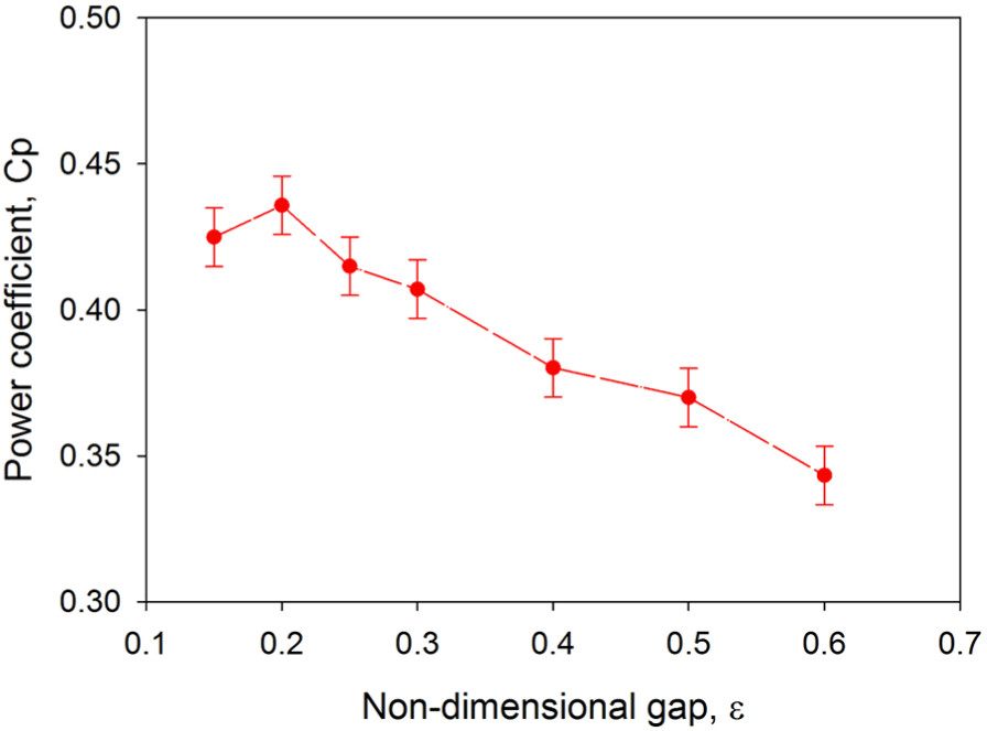
Comparison of the power coefficients obtained with various gaps $(r_{o} / r_{w} = 3.75, β = 0 °)$ .

The best performance of the VAWT was obtained when the gap was set to $ε = 0.2$ , as shown in Figure 13. Based on a gap of $ε = 0.2$ and an outer radius of $r_{o} / r_{w} = 3.75$ , only the relative angles $(β)$ of the guide wall were varied. Figure 14 shows the variation in the power coefficients with the relative angles. All of the computed power coefficients were larger than the power coefficient of 0.261, which was obtained without the wind tower. Therefore, this wind tower configuration will always enhance the output power of the VAWT.

Figure 14.

Comparison of the power coefficients obtained with various relative angles $(r_{o} / r_{w} = 3.75, ε = 0.2)$ .

Comparison of flow structures

Depending on the two design parameters ( $ε$ and $β$ ), various VAWT output powers were obtained. The maximum output power was obtained with $ε = 0.2$ and $β = 0 °$ , and the minimum output power was obtained with $ε = 0.5$ and $β = 25.71 °$ . In order to investigate the cause of these different results, they were compared with the results obtained without the wind tower. Figure 15 shows the relative streamlines and the static pressure contours together when a blade was located at $θ = 127 °$ . Figure 15(a) shows the velocity vectors and the relative flow direction on the stagnation point on the blade when the larger torque was obtained with $ε = 0.2$ and $β = 0 °$ . The large torque was created because the second guide wall located at $β = 51.41 °$ forced an upstream wind to flow toward the center of the wind tower. This wind direction increased the angle of attack and it contributed to the creation of a large torque.

Figure 15.

Comparison of the streamlines and the relative static pressure contours at $θ = 127 °$ : (a) with $β = 0 °, ε = 0.2$ ; (b) without wind tower; and (c) with $β = 25.71 °, ε = 0.5$ .

Figure 15(c) shows the velocity vectors when a smaller torque was obtained with $ε = 0.5$ and $β = 25.71 °$ . The angle of attack was smaller than that obtained without the wind tower. The first guide wall located at $β = 25.71 °$ forced the wind toward the center of the wind tower, but the wind distorted toward the rotational direction as soon as it passed the guide wall. This phenomenon occurred because there was a sufficient gap $(r_{i} - r_{w})$ so that the wind diverted to the side of the VAWT. Hence, this diversion resulted in the smaller angle of attack. Thus, the torque was less than that obtained without the wind tower. If the gap was reduced from $ε = 0.5$ to $ε = 0.2$ , the wind passing the first guide wall had the effect of increasing the angle of attack because the gap was too narrow to divert. From these results, it was revealed that the torque greatly depended on the relative flow velocity.

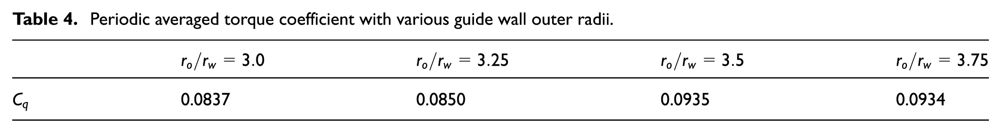
The outer radius parameter $(r_{o})$

In an equal upstream flow condition, a larger wind tower cannot receive a higher wind flow rate unless the total pressure of the wind is increased. The more the outer radius of the wind tower is increased, the greater the static pressure is increased. The increased static pressure results in a low velocity at the inlet of the wind tower compared with the wind velocity in the far field. In the case of $r_{o} / r_{w} = 3.75$ , the mass-averaged velocity was decreased by 10% in front of the wind tower due to the blockage. Hence, a computation was performed by changing only the outer radius of the wind tower on the condition that the maximum output power was obtained with $ε = 0.2$ and $β = 0 °$ . Table 4 shows the periodic averaged torque coefficients for the various outer diameters. The maximum output power was obtained with $r_{o} / r_{w} = 3.5$ . However, the outer radius had an insignificant effect on the output power compared with the other parameters.

Table 4.

Periodic averaged torque coefficient with various guide wall outer radii.

	$r_{o} / r_{w} = 3.0$	$r_{o} / r_{w} = 3.25$	$r_{o} / r_{w} = 3.5$	$r_{o} / r_{w} = 3.75$
$C_{q}$	0.0837	0.0850	0.0935	0.0934

Conclusion

A numerical study was conducted to improve the performance of the VAWT using a wind tower. The appropriate number of guide walls was determined to be seven based on an experiment. A transient analysis with a reduced computational domain was adopted and was validated using experimental results from the literature. Three parameters of the guide wall were selected as the major design variables. The output powers of the VAWT obtained with the various parameters are compared, and the correct configuration of the wind tower was investigated. The performance of the VAWT was mainly improved by the diversion of wind passing the guide wall within the wind tower. When the wind tower was designed with a gap of $ε = 0.2$ and an outer radius of $r_{o} / r_{w} = 3.5$ , the output power of the VAWT was always better than that obtained without the wind tower in an omnidirectional wind. When the wind came parallel to a guide wall, the maximum power coefficient was enhanced by 67%.

Footnotes

Handling Editor: Bo Yu

Declaration of conflicting interests

The author(s) declared no potential conflicts of interest with respect to the research, authorship, and/or publication of this article.

Funding

The author(s) disclosed receipt of the following financial support for the research, authorship, and/or publication of this article: This research was supported by “the renewable energy innovation project” of the Korea Institute of Energy Technology Evaluation and Planning (KETEP) that was granted financial resource from the Ministry of Trade, Industry & Energy, Republic of Korea. This financial support was gratefully acknowledged.

References

Tangler

Somers

. NREL airfoil families for HAWTs. In: Proceedings of the windpower ’95, Washington, DC, 26–30 March 1995, pp.117–123. Golden, CO: National Renewable Energy Laboratory.

Björk

. Coordinates and calculations for the FFA-W1-xxx, FFA-W2-xxx and FFA-W3-xxx series of airfoils for horizontal axis wind turbines. FFA TN 1990-15, 1990. Stockholm: The Aeronautical Research Institute of Sweden.

Fuglsang

Bak

. Design and verification of the new Risø-A1 airfoil family for wind turbines. In: 20th 2001 ASME wind energy symposium, Reno, NV, 11–14 January 2001, AIAA-2001-0028. Reston, VA: American Institute of Aeronautics and Astronautics.

Timmer

Rooij

RPJOM

. Summary of the Delft university wind turbine dedicated airfoils. In: 41st aerospace sciences meeting and exhibit, Reno, NV, 6–9 January 2003, AIAA-2003-0352. Reston, VA: American Institute of Aeronautics and Astronautics.

Grasso

. Hybrid optimization for wind turbine thick airfoils. In: 53rd AIAA/ASME/ASCE/AHS/ASC structures, structural dynamics and materials conference, Honolulu, HI, 23–26 April 2012, AIAA 2012-1354. Reston, VA: American Institute of Aeronautics and Astronautics.

Schubel

Richard

Crossley

. Wind turbine blade design. Energies 2012; 5: 3425–3449.

Colley

Mishra

. Computational flow field analysis of a vertical axis wind turbine. In: International conference on renewable energies and power quality (ICREPQ ’11), Las Palmas de Gran Canaria, 13–15 April 2011. Huddersfield: University of Huddersfield.

Park

Lee

Sabourin

. A novel vertical axis wind turbine for distributed & utility deployment. Ontario Sustainable Energy Association, http://citeseerx.ist.psu.edu/viewdoc/download?doi=10.1.1.500.9253&rep=rep1&type=pdf (2007, accessed 1 June 2017).

Kim

Song

et al . An experimental study on the performance of the vertical axis wind turbine. J Fluid Mach 2007; 10: 17–24.

10.

Takao

Kuma

Maeda

et al . A straight-bladed vertical axis wind turbine with a directed guide vane row—effect of guide vane geometry on the performance. J Therm Sci 2009; 18: 54–57.

11.

Chen

Ponta

Lago

. Perspectives on innovative concepts in wind-power generation. Energy Sustain Dev 2011; 15: 398–410.

12.

Park

Jung

Lee

et al . A new building-integrated wind turbine system utilizing the building. Energies 2015; 8: 11846–11870.

13.

Isensee

Adgul-Razzak

. Modeling and analysis of diffuser augmented wind turbine. Int J Energy Sci 2012; 2: 84–88.

14.

Phillips

Flay

RGJ

Nash

. Aerodynamic analysis and monitoring of the Vortec 7 diffuser-augmented wind turbine. IPENZ Trans 1999; 26: 1.

15.

Phillips

Richards

Flay

. CFD modeling and the development of the diffuser augmented wind turbine. Wind Struct 2002; 5: 267–276.

16.

Chong

Fazlizan

Poh

et al . The design, simulation and testing of an urban vertical axis wind turbine with the omni-direction-guide-vane. Appl Energ 2013; 112: 601–609.

17.

Nobile

Vahdati

Barlow

et al . Unsteady flow simulation of a vertical axis wind turbine: a two-dimensional study. In: TSBE engineering doctorate conference, Reading, 2 July 2013, https://www.reading.ac.uk/web/files/tsbe/Nobile_TSBE_Conference_Paper_2013.pdf

18.

Strickland

. The Darrieus turbine: a performance prediction model using multiple streamtubes. SAND75-0431, 1975. Albuquerque, NM: Sandia National Laboratories.

19.

Paraschivoiu

. Double-multiple streamtube model for studying vertical-axis wind turbine. J Propul Power 1988; 4: 370–378.

20.

Nobile

Vahdati

Barlow

et al . Unsteady flow simulation of a vertical axis augmented wind turbine: a two-dimensional study. J Wind Eng Ind Aerod 2014; 125: 168–179.

21.

Mclaren

. A numerical and experimental study of unsteady loading of high solidity vertical Axis wind turbines. PhD Thesis, McMaster University, Hamilton, ON, Canada, 2011.

22.

Mohamed

. Performance investigation of H-rotor Darrieus turbine with new airfoil shapes. Energy 2012; 47: 522–530.

23.

Nobile

Vahdati

Barlow

et al . Dynamic stall for a vertical axis wind turbine in a two-dimensional study. In: World renewable energy congress, Linkoping, 8–13 May 2011, http://www.ep.liu.se/ecp/057/vol15/023/ecp57vol15_023.pdf

24.

Abraham

Mowry

Plourde

et al . Numerical simulation of fluid flow around a vertical-axis turbine. J Renew Sustain Ener 2011: 3: 033109.

25.

Zhang

Liang

Liu

et al . Aerodynamic performance prediction of straight-bladed vertical axis wind turbine based on CFD. Adv Mech Eng 2013; 013: 905379.

26.

Alaimo

Esposito

Messineo

et al . 3D CFD analysis of a vertical axis wind turbine. Energies 2015; 8: 3013–3033.

27.

Carrigan

Dennis

Han

et al . Aerodynamic shape optimization of a vertical-axis wind turbine using differential evolution. ISRN Renewable Energy 2012; 2012: 528418.

28.

Lanzafame

Mauro

Messina

. 2D CFD modeling of H-Darrieus wind turbines using a transition turbulence model. Energy Proced 2014; 45: 131–140.

29.

Mohamed

. Impacts of solidity and hybrid system in small wind turbines performance. Energy 2013; 57: 495–504.

30.

Zhu

et al . 2.5D large eddy simulation of vertical axis wind turbine in consideration of high angle of attack flow. Renew Energ 2013; 51: 317–330.

31.

CFX. Ansys CFX (Version 15). Canonsburg, PA, USA: ANSYS Inc., 2014.

32.

Castelli

Englaro

Benini

. The Darrieus wind turbine: proposal for a new performance prediction model based on CFD. Energy 2011; 36: 4919–4934.

33.

Howell

Qin

Edwards

et al . Wind tunnel and numerical study of a small vertical axis wind turbine. Renew Energ 2010; 35: 412–422.

34.

Takao

Maeda

Kamada

et al . A straight-bladed vertical axis wind turbine with a directed guide vane row. J Fluid Sci Technol 2008; 3: 379–386.

Numerical study to investigate the design parameters of a wind tower to improve the performance of a vertical-axis wind turbine

Abstract

Keywords

Introduction

Numerical method

Validation of numerical method

Comparison with Castelli’s results

Comparison with Howell’s results

Comparison with Takao’s results

Discussion of three comparison cases

Comparison between a 2.5D and a 3D computation

Wind tower and wind turbine

The relative angle parameter ( β )

The inner radius parameter ( r i )

Comparison of flow structures

The outer radius parameter ( r o )

Conclusion

Footnotes

Declaration of conflicting interests

Funding

References

The relative angle parameter $(β)$

The inner radius parameter $(r_{i})$

The outer radius parameter $(r_{o})$