Sage Journals: Discover world-class research

Abstract

Tramp shipping transport is an important part of ocean transportation. However, facing the spot market with many uncertain conditions, it is not easy for fleet operators to plan vessel’s routes and schedule in the later period time, especially considering the situation that loading time window for a lot of cargoes has strong randomness. This article designed a linear programming model with chance constraints for the time window of loading cargo. Before the optimization, a survey for the waiting time of ships for berths is carried out in some of the ports with large export volume. Combined with the degree of acceptance how long ship owners can wait for the berth, the uncertain time window constraints can be transformed into deterministic constraints. The model is solved by column generation optimization technique. The model and algorithm are verified by a case of Panamax bulker fleet planning in real market. The results show that the model and the algorithm proposed in the article can well work on large-scale problem and can achieve good precision. Also, via sensitivity analysis, we provide decision makers good reference to balance profit and risks coming from randomness.

Keywords

Tramp shipping ship routing and scheduling uncertainty column generation chance constraint

Introduction

With the development of the world economy and the increasing integration of the world, volume of international trade is increasing year by year. Bear the transport of goods between countries in the world, ocean shipping accounted for the absolute superiority of the number, about 90%¹ of the international trade goods shipped by ocean-going vessels. There are three main forms of international ocean transportation in the academic view: industrial transport, tramp shipping, and liner shipping. The statistical data show that tramp shipping, the cargo of which is in bulk liquid and dry bulk, always occupies the main market share. In the long term, the technical progress of tramp shipping and application of management decision technology have been lagged behind liner shipping. In order to improve the utilization ratio of ships and reduce the ballast running distance, it is necessary to optimize the planning of tramp shipping routes and schedule.

In tramp shipping, the ship owner or operator does not own the cargo but selects available cargoes to transport so as to maximize the profit. In some certain conditions, a ship owner or operator need to make a plan for a period like few months that at what sequence their ship to visit some specified cargoes with loading time windows. The position, hire, and loading time window of a cargo are known or part of above information is known in advance. We discuss the ship routing and scheduling problem in our article.

In the real market, with environmental condition changing time to time, there are many factors hard to know exactly which can affect the supply of cargoes. Although statistically speaking, there is a probability that there will be big volume cargo coming out in a relatively fixed active season, but it is still affected by uncertainties such as supply and demand in the trade market, transport market tonnage supplement, local political situation, and weather. The random loading time window in port is a regular uncertain condition which affects the result a lot for a ship planner to make decision. Without a fixed time window, it is not only uneasy to arrange when a ship is suitable to visit the cargo but also has chance to miss the later scheduled plan. That is why we think the study on the subject is quite important for ship planning work in real market. This article explored how to combine uncertain loading time window into fleet resources planning, which means how to get the ships’ routes and scheduling.

The contributions of this article are threefold. First, via waiting time for berth from some ports, we found that the ships’ waiting time fit some certain distributions in some ports. This finding can be well applied to solve chance-constrained programming model we introduced in the article. Second, most of the previous ship routing and scheduling problems are solved by heuristic algorithm which is not easy to find the exact best solution in reasonable time. In this article, we use column generation technique to solve a large-scale problem which can get exact best solution in reasonable time. Third, the uncertain loading time window is taken into account in the problem of ship’s routing and scheduling problem. This is a real situation which decision-makers usually to face in the area of ship planning. Our programming model provides a very practical reference for the shipping business enterprise.

The remaining of the article is organized as follows. Section “Literature review” introduces related works in the field of fleet routing and scheduling. The specific formulation of fleet routing and scheduling with constraints of chance is described in section “Fleet routing and scheduling problem based on constraints of chance,” while section “Algorithm” introduces the algorithm of the proposed model. Case study is fully described and solved in section “Case study” with sensitivity analysis and evaluation of algorithm. Finally, conclusions are drawn in section “Conclusion and future work” along with future work.

Literature review

In the field of fleet routing and scheduling research, how ships coordinate the demand for cargo transportation is an important issue in the transportation of industry and tramp vessels. One cargo is made up of the specified amount of the product to be extracted in the designated port, which is transported and unloaded at the designated unloading port. Because the exact time is important for loading,^2,3 there is often a time window in port of loading. Due to berth resource scarcity properties during this period, ships must begin the process of loading of the goods as soon as possible. There may also be unloading time window.

The ship operator of a tramp vessel focuses on maximizing the profit. Unscheduled ship operation plan operations usually have a set of mandatory contract goods and will try to increase the ships’ availability for transportation. We focus on the tramp ship planning and ship scheduling problem, because this field contains the most general situation. Most of the corresponding industrial transportation problems are also similar. The details of the problem we discuss here are similar to those described by people like Desrosiers et al.,⁴ which include a multi-car collection and delivery problem. Korsvik and Fagerholt⁵ offered a Tabu search heuristic algorithm, which is the opposite of the heuristics of people like Brønmo et al.,⁶ which allows for the infeasible solution window constraint on the capacity and time window of the ship. Tabu search heuristic is better than the local search heuristics model proposed by the people like Brønmo et al.,⁶ especially for larger and more constrained problems. In a recent paper, Malliappi et al.⁷ proposed a variable neighborhood search heuristic algorithm for a same problem. They have changed their strength to the standard issue of land transportation, due to the lacking of realistic data in the physical market of tramp shipping. They compared their own neighborhood search heuristic algorithms with Brønmo et al.⁶ and Korsvik et al.’s⁵ Tabu search heuristic algorithm. The results show that the average variable neighborhood search has the best heuristic algorithms of them.

Jetlund and Karimi⁸ studied a problem which is the choice of route selection and ship scheduling in bulk liquid chemicals in transportation areas of the Asia-Pacific region by a shipping operator. For their problem, the authors presented a mixed-integer linear programming (MILP) formulation using variable-length slots and proposed a heuristic decomposition algorithm that obtains the fleet schedule by repeatedly solving the base formulation for a single ship. The method has been got through the real case data test, which involved 10 oil tankers and 79 transport goods problems. The profit grew up 32.7% when compared with before experience assigned task.

In the most literature of tramp shipping, the cargo cannot exceed the loading capacity of the ships. By introducing decomposition plate load, the limit can be removed and the goods can be realized as partial shipments between several ships. This problem was learned by Andersson.⁹ Hennig et al.¹⁰ designed a general mathematical model to illustrate problem basis condition that cargo can be split. A feature of the problem is, compared to the previous discussion, that it has no predefined cargoes. Fagerholt¹¹ and Lindstad et al.¹² put forward the decision support system (DSS), and it is used for ship routing and scheduling optimization, in which many kinds of heuristic algorithms from Brønmo, Korsvik et al., Korsvik and Fagerholt are cooperated. The one important experience of system design emphasized the importance of DSS and user interaction, rather than focusing on the optimization algorithm.

For the larger size problem, DSS method become less effective. Therefore, Brønmo et al.¹³ recommended the use of dynamic column generation scheme, according to the need to generate a feasible course of the ship. Because they have to discrete quantity of goods, the solutions must be changed to a certain extent. The problem last converted into heuristic column generation method. Column generation is an optimization algorithm for solving large-size linear programming problem. This theory was first presented in 1960 by Dantzig and Wolfe.¹⁴ In 1961, Gilmore and Gomory¹⁵ applied this method in cutting model problem. In 1984, the method was applied in a problem of vehicle routing problem (VRP) with time window.¹⁶ Kobayashi and Kubo¹⁷ studied an industrial oil tankers transport routes and scheduling problem in the practical market. And, Potthoff et al.¹⁸ used the method for railway crew rescheduling problem. And, in recent years, this method is more and more taken to solve linear programming with exact solution.^19–22

As for the ship route planning and scheduling problem, many pure or MILP models and their extensions are developed, which can refer to these literatures.^23–31 Zeng and Yang³² combined integer programming with heuristics. Cho and Perakis,³³ considering the fleet size, mixing, and delivery route assignment, presented integer linear programming models over a long-term planning horizon. Jaramillo and Perakis³⁴ proposed an integer linear programming model with two feasible models based on mixed linear-integer programming models. Fagerholt³⁵ worked a three-phase method by assuming weekly liner routes for this fleet deployment problem. Yang et al.³⁶ proposed a mixed-integer programming model based on investment of multimode according to the transport demand and routes under the fluctuant market conditions. A genetic algorithm was presented by Lin and Liu³⁷ based on the actual operating problems to determine ship allocation. Xie et al.³⁸ proposed an algorithm using both the linear programming formulation and dynamic programming techniques to get a better solution compared with using linear model only in others’ liner models.

Mostly, fixed shipment demand and direct shipping transportation without transshipment are in above-mentioned papers. But in shipping reality, the demand in future is quite uncertain, which brought another parts of the literature.^39,40 Meng et al.⁴¹ proposed a solution method which combined a dual decomposition with Lagrangian relaxation method to integrate the sample average approximation (SAA) method under uncertain demand. Yang et al.⁴² established a mixed-integer programming model based on multiple influencing factors. In front of complicated future circumstance, Halvorsen-Weare et al.⁴³ put forward a solution algorithm and several robustness strategies with the uncertain problems.

Fleet routing and scheduling problem based on constraints of chance

Problem description

Problems are described as follows: a large dry bulk ship owner controls some of the ships around the world that need to plan routes in a certain future period. There are some cargoes with fixed information on the spot market to be chosen to transport. The information of loading and unloading ports, the loading time window, the expected voyage time, and hire income is known. There are also some cargoes with information of loading time window and hire unknown. The expected hire for these cargoes can be forecasted through experience and other market information. And, the ship owners will plan the routes for the ships they will put into the spot market based on the forecast results and other known information. Since whether berths are available for some cargoes is also random, it will take some time for the ships to wait after arriving at the loading port. The length of time to wait for the berthing varies with the time of arrival of the ship.

By sampling survey data in some ports which regularly have large volume of goods to export in seasonable time, we found there is a certain statistical regularity in the anchorage time. The waiting time for berths for ships’ interval to access the same port fits some probability distribution. We carried out surveys for waiting time for berths from some ports from which cargoes regularly come year by year, such as Jakarta in Indonesia, Goa in India, Paranagua in Brazil, Kwinana in Australia, New Orleans in the United States.

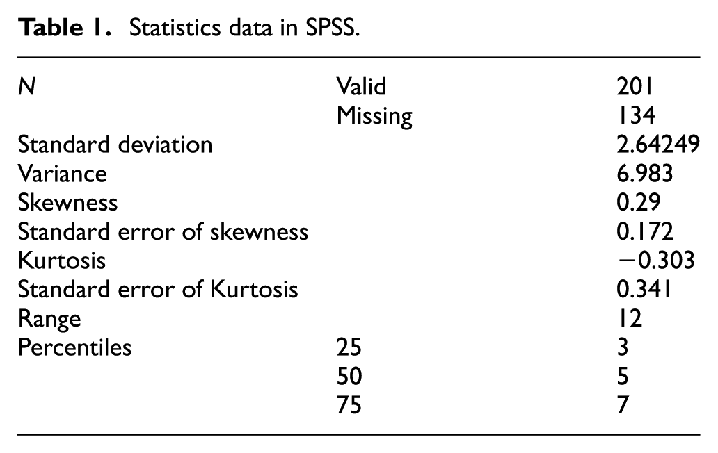
Take Jakarta as an example, we collected waiting time data of dry bulker arrived Jakarta from January to March in 2015. After times comparison, we found that when taking 6 h as time slice, the waiting time allows some known distribution and can pass hypothesis test. Figures 1 and 2 show berth time data and the hypothesis test by SPSS, respectively. From the data, we can concluded that from 1 January to 24 January, the waiting time for berth of ships arrived Jakarta is subject to a normal distribution of µ = 5.41 and σ = 2.64 (Tables 1 and 2).

Figure 1.

Waiting time for berth of dry bulkers arrived in Jakarta from January to March in 2015.

Figure 2.

Hypothesis test chart by SPSS.

Table 1.

Statistics data in SPSS.

N	Valid	201
	Missing	134
Standard deviation		2.64249
Variance		6.983
Skewness		0.29
Standard error of skewness		0.172
Kurtosis		−0.303
Standard error of Kurtosis		0.341
Range		12
Percentiles	25	3
	50	5
	75	7

Table 2.

One-sample Kolmogorov–Smirnov test.

		VAR00001
N		201
Normal parameters^a,b	Mean	5.408
	Standard deviation	2.64249
Most extreme differences	Absolute	0.088
	Positive	0.088
	Negative	−0.066
Kolmogorov–Smirnov Z		1.247
Asymptotic significance (two-tailed)		0.089

Test distribution is normal.

Calculated from data.

Similar to the above process, we sampled statistics and analyzed the ship’s berth data for Goa in India, the US Bay Area, Paranagua in Brazil, Kwinana in Australia, and Yosu in Korea, total of five commonly used export ports. The statistics pattern will help us to deal with the uncertain loading time window in these ports.

Model formulation

Via the problem description, we can see for each ship there are a series of cargoes to visit in strict accordance with the loading time window. Thus, in practice, very few decision-makers will venture to arrange ships to visit cargoes that are likely to miss time windows. And those cargoes with random time window also add the risk that the ships to miss the later schedule after visiting them. In the model, we designed the loading time window of some cargoes to meet certain confidence in a certain area constraints. Then, use chance-constrained programming model to solve this problem. Before giving the established model, notations used in this article are listed as follows:

N: a collection of all nodes in the problem;

$N^{O}$ : the virtual starting point of all ships, $N^{O} = {o}$ ;

$N^{S}$ : a collection of actual starting points of all ships, $N^{S} = {1, 2, \dots, k}$ ;

$N^{I}$ : a collection of all cargo, $N^{I} = {1, 2, \dots, n}$ ;

$N^{D}$ : the virtual destination point of all ships, $N^{D} = {d}$ ;

$N^{m}$ : a collection of cargoes affected by the delay of the ship;

$N^{ms}$ : a collection of cargoes affected by the delay of the ship;

$E (W_{ijk})$ : the expected income for the duration that from the Vessel k arrive point i till traveling to arrive the point j; $\forall i \in N^{O} \cup N^{S} \cup N^{I}, \forall j \in N^{S} \cup N^{I} \cup N^{D}$ , $\forall k \in V$ ;

$C_{ijk}$ : the total cost of ship k from the time she leaves point i until arrives at point j, $\forall i \in N^{O} \cup N^{S} \cup N^{I}, \forall j \in N^{S} \cup N^{I} \cup N^{D}$ , $\forall k \in V$ ;

$C_{0}^{k}$ : the fixed cost of ship k for daily operation, $\forall k \in V$ ;

$W_{ms}^{q}$ : income what the cargo missed the time window originally should have generated, $\forall q \in N^{ms}$ ;

$β$ : penalty factor the ship has missed the time window;

$α_{jk}$ : the probability of the ship k meets the time window of the cargo j, $\forall j \in M, \forall k \in V$ ;

$l_{j}$ : the number of ships returned to the operating area j at the end of a calculation cycle;

Q: the maximum days of waiting for berth which ship owner can accept;

S: a collection of actual starting points of all ships, $S = {1, 2, \dots, k}$ ;

$x_{ijk}$ : 1 if ship k services cargo node i immediately before cargo node j, 0 otherwise.

The following models are established

\begin{matrix} MAX = \sum_{k \in V} \sum_{i \in N} \sum_{j \in N} E (W_{ijk}) x_{ijk} - \sum_{k \in V} \sum_{i \in N} \sum_{j \in N} C_{ijk} x_{ijk} \\ - \sum_{k \in V} C_{0}^{k} - \sum_{q \in N^{ms}} β W_{ms}^{q} \end{matrix}

(1)

Subject to

\sum_{i \in S} x_{oik} = 1, \forall k \in V

(2)

\sum_{j \in N} x_{ijk} = 1, \forall i \in S

(3)

\sum_{i \in N} x_{ijk} = \sum_{i' \in N} x_{ji' k}, \forall j \in N, \forall k \in V

(4)

\sum_{j \in N} \sum_{k \in V} x_{ijk} \leq 1, \forall i \in N

(5)

\sum_{k \in V} \sum_{i \in N} x_{i, d_{j}, k} \geq l_{j}, \forall i \in N

(6)

\sum_{j \in F} l_{j} = k

(7)

\begin{matrix} \Pr (x_{ijk} \times (τ_{k}^{i} + t_{ij} - t_{j}^{latest}) \leq 0) \geq α_{jk}, \\ \forall i \in N^{I}, \forall j \in N^{m}, \forall k \in V \end{matrix}

(8)

\begin{matrix} \Pr (x_{ijk} \times (τ_{k}^{i} + t_{ij} + t_{j}^{w} - t_{j}^{earliest}) \geq 0) \geq α_{jk}, \\ \forall i \in N^{I}, \forall j \in N^{m}, \forall k \in V \end{matrix}

(9)

\Pr (t_{j}^{w} \leq Q) \geq α_{jk}, \forall j \in N^{m}, \forall k \in V

(10)

\sum_{j \in N^{m}} x_{ijk} \leq K, \forall k \in V

(11)

\begin{matrix} x_{ijk} \times (τ_{k}^{i} + t_{ij} - t_{j}^{latest}) \leq 0, \\ \forall i \in N^{I}, j \in N^{I} \ N^{m}, \forall k \in V \end{matrix}

(12)

\begin{matrix} x_{ijk} \times (τ_{k}^{i} + t_{ij} + t_{i}^{w} - t_{j}^{earliest}) \geq 0, \\ \forall i \in N^{I}, j \in N^{I} \ N^{m}, \forall k \in V \end{matrix}

(13)

\sum_{\forall i, j \in N} \frac{x_{ijk} \times d_{ij}}{v'} + x_{ijk} \times (t_{j}^{w} + t_{j}^{dur}) \leq t_{s}^{\lim}

(14)

x_{ijk} \in {0, 1}, \forall i \in N, \forall j \in N, i \neq j, \forall k \in V

(15)

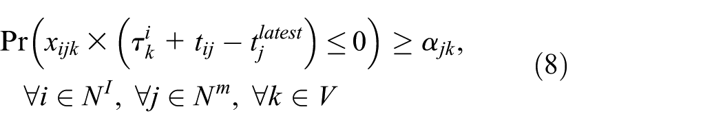
This objective represents the maximum profit for all operating vessels throughout the operation period. The four sub-items represent the income of all shipments of goods, the variable costs of all shipments, the fixed costs of all vessels, and the additional costs if a vessel missed the time-window. Constraint (2) indicates that all ships arrive from the virtual point to the actual starting point of the ship. Constraint (3) means that all ships are accessible from the starting point and can only visit one cargo. Constraint (4) indicates that the total number of ships entering and leaving the ship is consistent. Constraint (5) means that all cargoes are accessed by up to one ship. Constraint (6) represents the number of constraints on the number of ships returned to the area. Constraint (7) indicates that the number of ships returning to the end of all areas is equal to the total number of ships. Constraint (8) and constraint (9) represent constraints on the time at which the ship arrives at port of loading of the cargo. Constraint (10) indicates that the least confidence level that a decision can accept their vessels’ longest waiting time. Constraint (11) indicates that each ship has a maximum number of points that have randomness. Constraints (12) and (13) indicate that the paddock time is not random and the cargo load time window is constrained. Constraint (14) represents the ship’s total operating time constraint on any r-path. Constraint (15) indicates that the decision variable is 0 or 1; the decision variable is 1 when the cargo ships are accessed; otherwise, 0.

The opportunity constraint $\Pr (t_{j}^{w} \leq Q) \geq α_{jk}, \forall j \in M, \forall k \in V$ . $t_{j_{i}}^{w} ~ F (λ_{i}), i \in TP$ is used to describe the randomness of the waiting time after the arrival of the ship, indicating the probability of distribution of the pallet on the first time fragment for the randomness of the waiting time. The traditional method for the chance-constrained programming is according to the given confidence level, first to convert chance constraints into their respective certainty equivalence class, then to solve by the traditional method of the equivalent deterministic models. In some special cases, the chance-constrained programming problem can be converted into deterministic mathematical programming problem. But for more complex chance-constrained programming problems, such as the objective function is a high order function. That chance constraints cannot be transformed into deterministic conditions by using traditional method. In this article, we need to identify whether the loading time window is stochastic. Via the collected data of the ship’s waiting time, we need to test if it has a uniform distribution. These stochastic constraints can be transformed into deterministic problems for further study if the known statistic laws are known in the actual data.

Algorithm

To solve the problem, first we transform the original model into set partitioning problem (SPP) model. Then, the solution steps are as follows:

Step 1. For the conditional probability constraint, with the known sampling data, we can determine its probability density function and parameters.

Step 2. The conditional probability constraint is transformed into a deterministic constraint according to the calibrated probability density function.

Step 3. For the inability to fit the data, we inquire the known statistical data according to the conditional probability constraint directly, and the conditional probability constraint is transformed into the deterministic constraint by the statistical experience.

Step 4. Construct the initial set of columns to form the initial restricted main problem (RMP).⁴⁴

Step 5. Solve the RMP, get the corresponding dual problem.

Step 6. Solve the sub-problem, using the interpolation method to obtain the initial feasible solution.

Step 7. Get the path r to improve the subjective problem.

Step 8. Cycle the above steps until the main problem can no longer be improved to get the optimal solution.

Combined with the above process, the problem can be solved.

Case study

Case description and results

In this section, we choose a practical case to calculate and discuss the verification results of the planning model and algorithm proposed in this article for large-scale practical problems. Taking the Panamax dry bulk fleet of a large state-owned ocean-going shipping company in China as an example, the article uses the mathematical model established above to study the market situation in the future for a period of time and will focus on how to plan the routes and schedule of the fleet in order to make the whole fleet achieve maximum profit during the planning period.

A large shipping company is mainly engaged in dry bulk ocean shipping business. The company manages a fleet of more than 100 vessels including cape size, Panamax, and handy size. There are a total of 22 own and hired ships operating in Panamax fleet. In this case, we select Panamax fleet operations as an example for analysis. In all 22 ships, 5 of them are in a state of long-time charter, and the remaining 17 ship contains 12 ships which need to return to Shanghai, China, for repair or inspection or to be return to the head owner when current charter party expired within a year (in calculation, we take the shortest operation time constraints for 300 days, the longest run time constraints for 360 days). These vessels cannot be in a long-time charter for more than 1 year. The position and age of each ship are introduced in Table 3. We assume that the hires of candidate cargo are known or can be predicted. The distance matrix of all points is shown in Table 4. Some of the cargoes have random idle time at loading port with which the probability distribution is known.

Table 3.

Vessels’ position and age.

Vessel	Age of vessel (years)	Berthing port	Maximum operating time (days)
Vessel 1	4	Dalian	360
Vessel 2	3	Shanghai	360
Vessel 3	7	Yokohama	360
Vessel 4	5	Singapore	360
Vessel 5	2	Chennai	360
Vessel 6	8	Durban	360
Vessel 7	10	Cape Passero	360
Vessel 8	3	Houston	360
Vessel 9	6	Santos	360
Vessel 10	1	New Orleans	360
Vessel 11	2	Bayuquan	360
Vessel 12	5	Vizag	360
Vessel 13	4	Tubarao	540
Vessel 14	2	Beihai	540
Vessel 15	3	Shimizu	540
Vessel 16	1	Tema	540
Vessel 17	2	Tubarao	720

Table 4.

Distance matrix of all points (unit: days).

		Vessel 1	Vessel 2	…	Cargo 1	…	Cargo 93	Cargo 94
		Dalian	Shanghai	…	Xiamen	…	Lianyungang	Tianjin
Cargo 1	Tianjin	1	1		2		1	0
Cargo 2	Longkou	1	1		2		1	1
…		…		…	…	…	…
Cargo 3	Vanino	3	4	…	6	…	4	3
Cargo 93	Constanta	30	29		29		29	30
Cargo 94	Jubail	12	11		11		11	12
Destination	Shanghai	2	0		2		1	2

Assume that the ship owner is expected to put the ship into three strategic operations:

Strategy 1. A 1-year time charter or sign contract of cargoes with duration period about 1 year.

Strategy 2. A 6 months time charter or sign contract of cargoes with duration period about 6 months.

Strategy 3. Spot market operation; wait for a number of months before making later decisions.

Finally, owners decide that two ships will be put into the strategy 1, 5 ships (Vessels 11–15) in strategy 2, and 10 ships (Vessels 1–10) in strategy 3. For vessel 16 and vessel 17 which will be put into strategy 1, the 1-year daily hire is US$7250. For ships that put into Strategy 2, the actual 2 ships, vessel 14 and vessel 15, will carry out 6 months period with US$8250 as hire. Vessels 11–13 will sign a period of about 4–6 months of cargoes contract. And vessels 1–10 will be put into strategy 3, which is our focus to discuss how to plan their route and scheduling to visit cargoes.

The next step is to carry out the route planning and scheduling plan according to the known information on the market for vessel 1–10. For 10 ships on the spot market, it is divided into two stages to optimize, the first phase of the planning period is 135–195 days, taking into account the total operating time of the ships 280–360 days, and the implementation of one cargo duration of 30–100 days or so, so the first phase of the planning period span is relatively wide. Otherwise, it is difficult to get a higher profitability of the solution. When the first planning period is about to end, the Atlantic Ocean and the Pacific Ocean should have at least three vessels in their area to ensure the balance of the ship’s configuration in the world. At this stage, we take the penalty factor as 0.8 to express the cost for missing the loading time window. For a cargo with a random loading time window, the maximum waiting time for the ship to accept the ship is 10 days and the confidence level is 70%. The information on the cargo of the 10 vessels is shown in Appendix 1. After calculation, there are four orders in the cargoes which have random loading time window not in accordance with the owner’s acceptable waiting time and are excluded from the candidate options.

The cargoes that fit the time probability constraints will be added directly to the candidate set for optimization. After the optimization path is obtained, the random number generator set will generate random waiting day’s number. After adding number of waiting days, if any of the loading time windows of later cargoes is missed, then the punishment factor is set to be active.

After the end of the first stage planning period, the investment strategy is redesigned for the 15 ships of strategy 2 and strategy 3. The calculation shows seven ships should be put into strategy 2 and eight ships into strategy 3. Vessels 11–15 in strategy 2 originally added vessel 2 and vessel 10 will be chartered out basis their balance about 6 months. The hire is US$6500. The remaining eight ships that are put into in strategy 3 are required to carry out the remaining time under the operating restriction. And the ships will return to the virtual endpoint in Shanghai after the operation is completed. The ship owner can accept the maximum waiting time for 10 days as well, the confidence level of 70% (Table 5).

Table 5.

Optimal routes of calculation.

	Routes to visit cargoes	Fully loaded (days)	Ballast (days)	Waiting for berth (days)	Fixed cost (USD)	Changeable cost (USD)	Revenue (USD)	Profit (USD)
Vessel 1	1–31–48–62–sh	242	13	67	1,288,000	1,735,600	6,600,000	3,576,400
Vessel 2	16(2)–40	150	10	31	764,000	1,036,000	3,900,000	2,100,000
Vessel 3	90^a(5)–85–47–63–sh	215	38	57	1,240,000	1,563,600	4,912,500	2,108,900
Vessel 4	4–28–54–93–sh	235	11	98	1,376,000	1,815,200	5,490,000	2,298,800
Vessel 5	37–84–65–30–94–sh	230	27	73	1,320,000	1,704,400	3,557,000	532,600
Vessel 6	58–68–89–10–sh	265	9	66	1,360,000	1,864,800	5,145,000	1,920,200
Vessel 7	43–19–83(2)–12–70(6)–92^a(2)–7(1)–sh	280	13	53	1,384,000	1,907,600	4,863,000	1,571,400
Vessel 8	86–6–82–15–13(6)–11(2)–71–8(1)–sh	210	30	78	1,272,000	1,608,000	2,462,500	−417,500
Vessel 9	61–14–26–18(6)–9–sh	245	25	38	1,232,000	1,652,000	5,352,500	2,468,500
Vessel 10	88–3–81(6)	95	11	47	612,000	771,200	1,007,500	−375,700
Total		2167	187	608	11,848,000	15,658,400	43,290,000	15,783,600
One vessel per day					4000	5286	14,615	5329

Indicates that the ship missed the time window of the cargo; (): the number inside indicates the random numbers that are generated by the specified distribution.

The total calculated optimal routes in two stages are shown in Table 5. From the table, we can see that average daily profit for one vessel is US$5329. Total 46 cargoes are selected to visit. Eleven cargoes with random loading time window out of total 90 suitable candidates are selected to visit. Among the 11 cargoes, only 2 countered the situation that cause vessel to miss their later cargo plan.

Sensitivity analysis

Risk and opportunity in the market always exist at the same time, and decision-makers with different business styles may make different choices in the same market situation. In this article, $α_{jk}$ indicates the probability that ships meet the cargo time window. The higher value means that a ship has better chance to meet the loading time window of a cargo. But at the same time, if a ship to choose higher probability to meet the time window, then she would have to accept smaller number of candidate cargoes to choose comparing with lower value of parameter $α_{jk}$ . In this section, we test our theoretical inferences by testing different parameter values.

We change the value of $α_{jk}$ to 90% and waiting time of ships to 3 days. For cargo randomness of idle time, take up waiting time for 10 days. At the confidence level of 90%, results remove cargoes 32, 41, and 53, compared with that of 70% confidence level. When the maximum waiting time is 3 days, cargoes 8, 11, 13, 18, 51, 66, 72, 76, 77, 81, 90, and 92 will be removed at 70% of confidence level. Furthermore, cargoes 16, 23, 25, and 70 will be removed at 90% confidence level when the maximum waiting time is 3 days.

The profits in four scenarios are shown in Figure 3. Through comparative analysis, we have a random cargo summary of the following characteristics.

Figure 3.

Average profit of one vessel for four different scenarios.

When the maximum waiting time is 10 days and the confidence level is 90%, the fleet average daily profit is the maximum. In this case, the fleet can choose a large scale of cargoes. In these three constraints, there is no case where the randomness of the waiting time causes the delay of the following tray. In this case study, we have given that if idle time subsequent cargo delay happens to randomness, then delayed cargo income can only be calculated at 80% and 20% of their income for alternative ships and penalty cost of replacement goods. These costs vary in practices and make a big difference, so taking different parameters of penalty coefficient may have different effects on the results.

We set the same largest accept idle time for all cargoes. But in the actual market, idle time has many differences in different ports, from only 1 or 2 days to 1 month or longer in busy season. Therefore, the general situation is that policymakers have different idle time limits for different cargoes.

Overall, different policymakers have different preferences for risk, and the longer time the ship in ports and a berth, the higher the need of material supply and ship maintenance cost. Therefore, decision-makers need to figure out suitable decision based on their operating conditions and the judgment for the follow-up market.

Conclusion and future work

To improve the decision-making quality of ocean shipping enterprises in the fleet routing and scheduling area, especially for the large-scale nonlinear programming problems in practice, this article designed a linear programming model with chance constraints for the loading time window. In this article, the ship berth time survey is carried out for some of the ports with large export volume. Combined with the degree of acceptance of the owner for the berth waiting time, the uncertain time window constraints can be transformed into deterministic constraints. The model is solved using the improved shortest path algorithm combined with the column generation optimization technique, which breaks the limitation of the heuristic methods. In this article, the application of the algorithm shows the strength of finding satisfied path in time and space transportation network.

Combining with the randomness of ship waiting time in practical problems, the model is with constraint of chance, which focuses on investigating and analyzing the characteristic of ships’ berth waiting time in some ports and in particular seasons. We focus on fleet routing and scheduling optimization problem in the field of the fleet planning practice considering the randomness of the ship’s idle time in ports.

The article also has some deficiencies to be improved, limited by the algorithm design and accuracy of algorithm. In the follow-up study, the author will focus on the following discussion to make the model conform to the actual market situation. The target function will be varied. The target function will be set by technical indexes such as ship idle time and ballasted ratio. The ship will be not homogeneous. Ships are divided by age, holding cost, deadweight ton, and seaworthiness cargo.

Footnotes

Appendix

Appendix 1

Relevant information of vessels and 94 cargoes.

	Position/loading port	Discharging port	Ready date/layday	Canceling day	Distribution	Duration (days)	Hire (USD)
Vessel 1	Dalian		1
Vessel 2	Shanghai		5
Vessel 3	Yokohama		12
Vessel 4	Singapore		7
Vessel 5	Chennai		22
Vessel 6	Durban		18
Vessel 7	Cape Passero		6
Vessel 8	Houston		11
Vessel 9	Santos		27
Vessel 10	New Orleans		20
Cargo 1	Tianjin	Xiamen	2	5		12	10,000
Cargo 2	Longkou	Lagos	2	5		150	8200
Cargo 3	Vanino	Shanghai	85	90		15	11,500
Cargo 4	Seattle	Busan	22	30		55	16,000
Cargo 5	Qinhuangdao	Lake Charles	22	30		95	8000
Cargo 6	Samarinda	Guangzhou	80	87		20	12,000
Cargo 7^a	Jakarta	Inchon	301	324	Normal (1.4, 0.6)	25	11,000
Cargo 8	Gladestone	Busan	300	307		25	12,000
Cargo 9	Newcastle	Yingkou	299	304		40	18,000
Cargo 10	Bunbury	Chittagong	299	304		50	14,000
Cargo 11^a	Kwinana	Shibushi	220	239	Normal (3.3, 1.2)	45	13,500
Cargo 12	Surabaya	Beihai	220	225		30	11,500
Cargo 13^a	Port Kelang	Kosichang	185	199	Normal (5.2, 2.6)	20	11,000
Cargo 14	Kosichang	Kaohsiung	160	170		25	11,000
Cargo 15	Kuantan	Bayuquan	150	160		35	12,000
Cargo 16	Bintulu	Goa	9	14		40	15,000
Cargo 17	Geraldton	Kandla	265	275		45	13,800
Cargo 18	Goa	Lianyungang	245	255		35	10,500
Cargo 19	Haldia	Ningbo	140	147		35	10,000
Cargo 20	Tianjin	Genoa	154	159		105	10,000
Cargo 21	Inchon	Istanbul	135	145		140	8500
Cargo 22	Shanghai	Rotterdam	102	107		105	8200
Cargo 23^a	Yosu	Owendo	311	335	Poisson (2.6)	140	8500
Cargo 24	Longkou	Manzanillo	105	110		85	10,500
Cargo 25	Surabaya	Goa	41	45		25	15,000
Cargo 26	Gove	Cebu	205	211		20	12,000
Cargo 27	Durban	Jebel Ali	80	90		40	14,000
Cargo 28	Jubail	Mumbai	99	104		20	10,000
Cargo 29	SW Pass	Haldia	70	80		110	34,000
Cargo 30	Amsterdam	Ningbo	205	210		85	21,000
Cargo 31	Poti	Mesaieed	40	50		70	28,000
Cargo 32	Santos	Dalian	270	280		85	31,000
Cargo 33	Santos	Bandar Abbas	165	175		85	26,000
Cargo 34	Puerto Cabello	Algiers	200	205		40	20,500
Cargo 35	Los Angeles	Beilun	305	315		45	16,500
Cargo 36	Newcastle	Masinloc	215	225		35	13,200
Cargo 37	Tanjung Bara	Qinzhou	20	30		25	11,500
Cargo 38	Narvik	Lake Charles	10	20		40	12,000
Cargo 39	Paranagua	Cebu	1	10		100	28,000
Cargo 40	Santos	Qingdao	88	98		110	30,000
Cargo 41	Newport News	Mumbai	30	40		125	24,000
Cargo 42	Norfolk	Vizag	20	30		120	28,000
Cargo 43	SW Pass	Busan	20	30		105	29,000
Cargo 44	Murmansk	Damietta	90	100		35	13,000
Cargo 45	Saint Petersburg	Haldia	100	110		110	26,000
Cargo 46	Riga	Naples	110	120		40	15,000
Cargo 47	Narvik	Dakar	120	130		50	18,000
Cargo 48	Liverpool	Conakry	130	140		40	17,000
Cargo 49^a	Paranagua	Tema	242	267	Normal (21.3, 7.7)	40	22,000
Cargo 50^a	SW Pass	Shanghai	293	310	Normal (8.5, 5.2)	60	30,000
Cargo 51^a	SW Pass	Gamba	10	28	Normal (4.2, 2.1)	60	24,000
Cargo 52	SW Pass	Port Said	175	195		80	16,000
Cargo 53^a	SW Pass	Tianjin	265	287	Normal (7.7, 4.2)	75	34,000
Cargo 54	SW Pass	Kosichang	150	160		110	31,000
Cargo 55	SW Pass	Jebel Ali	160	170		95	36,000
Cargo 56^a	Paranagua	Lagos	17	40	Normal (18.6, 6.4)	80	21,000
Cargo 57	Paranagua	Lome	180	190		85	22,000
Cargo 58	Paranagua	Chittagong	30	40		110	28,000
Cargo 59^a	Paranagua	Doha	275	299	Normal (23.6, 8.5)	55	38,000
Cargo 60	Santos	Durban	190	200		60	24,000
Cargo 61	Santos	Shimizu	20	30		125	30,000
Cargo 62	Santos	Haiphong	200	210		120	32,000
Cargo 63	Santos	Fangcheng	210	220		115	31,000
Cargo 64	Santos	Inchon	220	230		125	33,000
Cargo 65	Dampier	Kandla	115	122		55	14,500
Cargo 66^a	Kwinana	Karachi	30	47	Normal (2.2, 1.8)	65	15,000
Cargo 67	Port Lincoln	Fangcheng	230	240		60	14,000
Cargo 68	Adelaide	Yingkou	155	165		75	14,000
Cargo 69	Dampier	Kosichang	240	250		45	13,500
Cargo 70	Tianjin	Cebu	250	260		20	9500
Cargo 71	Qinhuangdao	Kaohsiung	260	270		15	10,000
Cargo 72	Longkou	Poti	237	244		65	9200
Cargo 73	Yantai	Lagos	270	280		110	6000
Cargo 74	Shanghai	Tema	175	185		115	7800
Cargo 75	Dangjin	Douala	280	290		110	8500
Cargo 76^a	Yosu	Lome	282	300	Poisson (4.7)	105	9000
Cargo 77^a	Yosu	Houston	97	114	Poisson (3.8)	75	7500
Cargo 78	Dangjin	Lake Charles	300	310		100	7500
Cargo 79	Inchon	Los Angeles	310	320		80	9000
Cargo 80	Busan	Veracruz	175	180		100	7500
Cargo 81^a	Goa	Port Kelang	92	135	Manual statistic	20	9500
Cargo 82	Mumbai	Xiamen	120	125		25	10,500
Cargo 83^a	Goa	Lianyungang	175	188	Manual statistic	30	11,200
Cargo 84	Goa	Bayuquan	65	70		30	11,000
Cargo 85	Goa	Shenzhen	52	57		25	10,500
Cargo 86	Vizag	Guangzhou	35	45		25	10,500
Cargo 87	Vizag	Shibushi	143	148		30	10,500
Cargo 88	Haldia	Busan	55	67		30	11,000
Cargo 89	Doha	Nantong	245	252		30	10,500
Cargo 90	Inchon	Singapore	5	10		35	9500
Cargo 91	Yuzhny	Nantong	265	270		85	17,000
Cargo 92	Surigao	Yantai	251	256		35	11,500
Cargo 93	Constanta	Lianyungang	300	307		50	20,000
Cargo 94	Jubail	Tianjin	315	320		35	10,200

Cargoes which have uncertain loading time window.

Handling Editor: Gang Chen

Declaration of conflicting interests

The author(s) declared no potential conflicts of interest with respect to the research, authorship, and/or publication of this article.

Funding

The author(s) disclosed receipt of the following financial support for the research, authorship, and/or publication of this article: This research was supported by Higher Education Development Fund (for Collaborative Innovation Center) of Liaoning Province, China (grant no. 20110116401), Liaoning Excellent Talents in University (LR2015008), and the Fundamental Research Funds for the Central Universities (YWF-16-BJ-J-40 and DUT16YQ104).

References

http://unctad.org/en/pages/publicationwebflyer.aspx?publicationid=1650

Song

Guan

et al . K-nearest neighbor model for multiple-time-step prediction of short-term traffic condition. J Transp Eng 2016; 142: 04016018.

Yao

Chen

Cao

et al . Short-term traffic speed prediction for an urban corridor. Comput Aided Civ Inf 2017; 32: 154–169.

Desrosiers

Dumas

Solomon

et al . Chapter 2 time constrained routing and scheduling. Handb Oper Res Manage Sci 1995; 8: 35–139.

Korsvik

Fagerholt

A tabu search heuristic for ship routing and scheduling with flexible cargo quantities. J Heuristics 2010; 16: 117–137.

Brønmo

Christiansen

Fagerholt

et al . A multi-start local search heuristic for ship scheduling: a computational study. Comput Oper Res 2007; 34: 900–917.

Malliappi

Bennell

Potts

CN.

A variable neighborhood search heuristic for tramp ship scheduling computational logistics. Lect Notes Comput Sci 2011; 6971: 273–285.

Jetlund

Karimi

IA.

Improving the logistics of multi-compartment chemical tankers. Comput Chem Eng 2004; 28: 1267–1283.

Andersson

A maritime pulp distribution problem. Inf Syst Oper Res 2011; 49: 125–138.

10.

Hennig

Furman

Kocis

et al . Crude oil tanker routing and scheduling. Inf Syst Oper Res 2011; 49: 153–170.

11.

Fagerholt

A computer-based decision support system for vessel fleet scheduling—experience and future research. Decis Support Syst 2004; 37: 35–47.

12.

Lindstad

Asbjørnslett

Strømman

AH.

Reductions in greenhouse gas emissions and cost by shipping at lower speed. Energ Policy 2011; 39: 3456–3464.

13.

Brønmo

Nygreen

Lysgaard

Column generation approaches to ship scheduling with flexible cargo sizes. Eur J Oper Res 2010; 200: 139–150.

14.

Dantzig

Wolfe

Decomposition principle for linear programs. Oper Res 1960; 8: 101–111.

15.

Gilmore

Gomory

RE.

A linear programming approach to the cutting stock problem. Oper Res 1961; 6: 1963.

16.

Desrosiers

Sournis

Desrochers

Routing with time windows by column generation. Networks 1984; 14: 545–565.

17.

Kobayashi

Kubo

Optimization of oil tanker schedules by decomposition, column generation, and time-space network techniques. Japan J Ind Appl Math 2010; 27: 161–173.

18.

Potthoff

Huisman

Desaulniers

Column generation with dynamic duty selection for railway crew rescheduling. Transp Sci 2010; 44: 493–505.

19.

Peng

Shan

Guan

et al . Stable vessel-cargo matching in dry bulk shipping market with price game mechanism. Transp Res E Log 2016; 95: 76–94.

20.

Zhang

Wang

Sun

et al . The sightseeing bus schedule optimization under park and ride system in tourist attractions. Ann Oper Res. Epub ahead of print 7 November 2016. DOI: 10.1007/s10479–016–2364–4.

21.

Branchini

Armentano

Morabito

Routing and fleet deployment in liner shipping with spot voyages. Transp Res C 2015; 57: 188–205.

22.

Woumans

De Boeck

Beliën

et al . A column generation approach for solving the examination-timetabling problem. Eur J Oper Res 2016; 253: 178–194.

23.

Yao

et al . Transit network design based on travel time reliability. Transp Res C Emer 2014; 43: 233–248.

24.

Meng

Wang

TS.

A chance constrained programming model for short-term liner ship fleet planning problems. Marit Policy Manag 2010; 37: 329–346.

25.

Gelareh

Meng

A novel modeling approach for the fleet deployment problem within a short-term planning horizon. Transp Res E Log 2010; 46: 76–89.

26.

Yao

et al . An improved particle swarm optimization for carton heterogeneous vehicle routing problem with a collection depot. Ann Oper Res 2016; 242: 303–320.

27.

Liu

Yuan

XM.

Tactical planning models for managing container flow and ship deployment. Marit Policy Manag 2011; 38: 487–508.

28.

Zhu

Cai

et al . Two-phase optimization approach to transit hub location—the case of Dalian. J Transp Geogr 2013; 33: 62–71.

29.

Wang

Meng

A note on liner ship fleet deployment. Flex Serv Manuf J 2011; 23: 422–430.

30.

Kong

Sun

et al . A bi-level programming for bus lane network design. Transp Res C Emer 2015; 55: 310–327.

31.

Hwang

H-S

Visoldilokpun

Rosenberger

JM.

A branch-and-price-and cut method for ship scheduling with limited risk. Transp Sci 2008; 42: 336–351.

32.

Zeng

Yang

ZZ.

Model integrating fleet design and ship routing problems for coal shipping. Lect Notes Comput Sci 2007; 4489: 1000–1003.

33.

Cho

Perakis

AN.

Optimal liner fleet routing strategies. Marit Policy Manag 1996; 23: 249–259.

34.

Jaramillo

Perakis

AN.

Fleet deployment optimization for liner shipping part 2. Implementation and results. Marit Policy Manag 1991; 18: 235–262.

35.

Fagerholt

Optimal fleet design in a ship routing problem. Int Trans Oper Res 1999; 6: 453–464.

36.

Yang

Xie

Huo

. Modeling fleet planning strategy based on multimode investment. In: Second international symposium on computational intelligence and design (ISCID ’09), Changsha, China, 12–14 December 2009, pp.493–496. New York: IEEE.

37.

Lin

Liu

HY.

Combined ship allocation, routing and freight assignment in tramp shipping. Transp Res E Log 2011; 47: 414–431.

38.

Xie

Wang

Chen

DS.

A dynamic model and algorithm for fleet planning. Marit Policy Manag 2000; 27: 53–63.

39.

Meng

Wang

SA.

Liner ship fleet deployment with week-dependent container shipment demand. Eur J Oper Res 2012; 222: 241–252.

40.

Wang

et al . Liner ship fleet deployment with uncertain demand. Transp Res Rec 2014; 2409: 49–53.

41.

Meng

Wang

SA.

Short-term liner ship fleet planning with container transshipment and uncertain container shipment demand. Eur J Oper Res 2012; 223: 96–105.

42.

Yang

Zhang

Sang

et al . Mathematical approach for fleet planning under complicated circumstances. J Shanghai Jiaotong Univ 2014; 19: 241–250.

43.

Halvorsen-Weare

Fagerholt

Rönnqvist

Vessel routing and scheduling under uncertainty in the liquefied natural gas business. Comput Ind Eng 2013; 64: 290–301.

44.

Solomon

MM.

Algorithms for the vehicle routing and scheduling problem with time window constraints. Oper Res 1987; 35: 254–265.