Sage Journals: Discover world-class research

Abstract

This article proposes a new model to address the design problem of a sustainable regional logistics network with uncertainty in future logistics demand. In the proposed model, the future logistics demand is assumed to be a random variable with a given probability distribution. A set of chance constraints with regard to logistics service capacity and environmental impacts is incorporated to consider the sustainability of logistics network design. The proposed model is formulated as a two-stage robust optimization problem. The first-stage problem before the realization of future logistics demand aims to minimize a risk-averse objective by determining the optimal location and size of logistics parks with CO₂ emission taxes consideration. The second stage after the uncertain logistics demand has been determined is a scenario-based stochastic logistics service route choices equilibrium problem. A heuristic solution algorithm, which is a combination of penalty function method, genetic algorithm, and Gauss–Seidel decomposition approach, is developed to solve the proposed model. An illustrative example is given to show the application of the proposed model and solution algorithm. The findings show that total social welfare of the logistics system depends very much on the level of uncertainty in future logistics demand, capital budget for logistics parks, and confidence levels of the chance constraints.

Keywords

Regional logistics network sustainability logistics demand uncertainty two-stage robust design chance constraint genetic algorithm

Introduction

There is a wide consensus that freight transportation is a major contributor to climate change and global warming is due to various pollution emissions. Freight transportation is largely driven by fossil fuel combustion, mostly diesel fuel, resulting in emissions of greenhouse gases (GHG), such as carbon dioxide (CO₂), nitrogen oxide (NOx), sulfur oxide (SOx), particulate matters, and air toxics.¹ It is estimated that freight transport accounts for around 10% of energy-related carbon emissions.²

Therefore, it is clearly an urgent need for effective measures and policies to combat further environmental damage due to increased vehicular pollution emissions and to develop sustainable, low-carbon regional logistics systems.

Logistics network design is an important component of regional logistics system. It is normally viewed as a strategy planning problem, involving logistics facility planning and sustainable logistics management policy-making. To determine the optimal number and size of logistics parks is a core task of logistics facility planning, while the sustainable logistics management policy mostly refers to CO₂ emission taxes.^3,4

A logistics park, which is also referred to as “logistics village” in Germany, “distribution park” in Japan, and “logistics platform” in Spain, is a specially important component of the regional logistics network. A logistics park implies a spatial concentration area for grouping various activities, such as transportation, distribution, warehousing, commercial trade, and other related services (such as maintenance and repair). It is also an intersection of different transport modes and an interface between local traffic and long-distance traffic.⁵

Logistics parks play an important role in promoting logistics efficiency, decreasing the logistics operation cost, as well as environmental effects (e.g. reducing CO₂ emissions and air pollution) due to economics of scale with logistics clusters.^6,7 Economy of scale regarding the construction of logistics parks refers to the phenomenon that the average construction cost per unit area for a logistics park decreases with the increase in the size of the logistics park.^8–10 Meanwhile, the economies of scale regarding the operation of logistics parks refer to the phenomenon that average operating cost per unit of shipment decreases with the increase in the size of the logistics park due to the clustering and synergetic effects among the different logistics service providers.^11,12 However, it would lead to lower utilization rate of logistics facilities and higher logistics operation cost due to less considering logistics choice behavior and logistics parks collaboration configures.¹³

Meanwhile, the sustainable regional logistics network design will face the below two challenges. The total volume and structure of logistics demand retain both change due to population aggregation and industrial reconstruction. And the higher energy consumption and lower efficiency on city logistics have always take place due to the lack of system integration and less consideration of economics of scale economy on logistics system. Therefore, it is vital for authorities to optimize logistics network design so as to build a sustainable logistics network with low-carbon and higher logistics operator efficiency.

An important task of regional logistics network design is to determine the optimal location and size of different logistics terminals (especially logistic parks) and the corresponding configure patterns.¹⁴ Among the configure patterns of regional logistics network design, the configure pattern based on hub-and-spoke structure is applied widely.¹⁵ Soysal et al.¹⁶ presented a network model of wagonload traffic, which aimed to determine the hub location and size considering total cost and efficiency of the network system. Vieira et al.¹⁷ investigated a hub location problem from the perspective of network design, jointly considering the transportation cost and travel time, and proposed a mixed-integer programming formulation. Crainic et al.¹⁸ addressed a two-tiered freight distribution system in a big city, aiming to determine the optimal locations of logistics facilities.

The classic network design model based on hub-and-spoke can well describe the economics of scale by transportation consolidation, but there exists deficient in characterizing the interactive decision relationship among different shareholders. Harker and Friesz¹⁹ reviewed the major modeling techniques that had been applied in analyzing intercity freight network equilibrium, and pointed out the shortcomings of the spatial price equilibrium models. Taniguchi et al.²⁰ proposed a bi-level model to determine the optimal size and location of public logistics terminals and solved the model using queuing theory and nonlinear programming techniques. Catalano and Migliore²¹ presented an optimal model on design of logistic terminals based on Stackelberg game, which aimed to determine the optimal location pattern and public share in investments. The finding shows that the transhipment and consolidation services should be concentrated at few terminals to exploit fully economies of scale at the expense of the average travel time to reach the logistic platforms.

The research mentioned above has primarily been concentrating on problems of a static, deterministic nature. However, the regional logistics network planning involves a longer time span range from 5 to 20 years depending on the construction project, in which the logistics demand often preserves some uncertainty due to the change in regional economic and industrial structure.²² Optimal solutions for a deterministic problem may turn out to have poor quality or even lose feasibility as a result of uncertain factors.²³

Therefore, uncertainty (particularly, uncertain demands) in logistics network design is one of the most challenging issues. Stochastic optimization and robust optimization are the two main paradigms for dealing with uncertainty in mathematical programming models. Stochastic optimization relies on the distribution of the uncertain parameters while robust optimization is a distribution-free approach aiming to find the worst case scenario with respect to a predefined uncertainty set.^24,25

Lium et al.²⁶ presented an optimization model of stochastic service network design, which is an extension of the classic multi-period service network design model by introducing stochastic demand in the form of a scenario tree. A mixed-integer programming model was developed with the objective of minimizing the expected cost over all scenarios. Hoff et al.²⁷ is the continuation of Lium et al.,²⁶ with the primary aim of developing efficient approaches that can solve large real-sized instances. A variable neighborhood search (VNS)-based approach was proposed. Yang and Chen²⁸ investigated a two-stage stochastic model for the air freight network design problems with uncertain demand. The top-level decision variables of this problem include the number and location of air freight hubs, while the second stage consists of decisions of flight routes and flows. Ukkusuri and Patil²⁹ developed a multi-period network design problem considering both demand uncertainty and demand elasticity and presented a bi-level stochastic mathematical programming with complementarily constraints. The finding shows that under demand uncertainty, there are potential benefits of introducing flexibility in investment decisions.

Plastria³⁰ considered the problem of expanding arc capacities in a network subject to demand and travel time uncertainty and proposed a robust optimization model that is insensitive to this uncertainty. MT Melo et al.³¹ addressed the robust optimization model based on scenario-based stochastic mixed-integer programs for infrastructure network under stochastic arc disruption and gave a cutting-plane algorithm and several heuristic approaches for solving the optimal models. Mittal et al.³² addressed the optimal inland-empty-container depot locations under stochastic demand, presenting a two-stage stochastic analysis model. Chen and Fan³³ presented a stochastic programming model to cope with uncertainty brought by cellulosic ethanol technology evolvement in transportation fuel portfolio design problems. De Rosa et al.³⁴ studied a new robust formulation for strategic location and capacity planning considering potential company acquisitions under uncertainty. They found that robust model achieves superior results to the deterministic configurations in exhaustive computational tests. For comprehensive surveys on robust optimization, the readers are referred to Gabrel et al.³⁵ and Kamruzzaman and Hine.³⁶ Mohammadi et al.³⁷ addressed the sustainable hub location problem with uncertain data, in which two new environmental-based cost functions accounting for air and noise pollution of vehicles are incorporated. And a mixed stochastic programming model is proposed and the solution based on simulated annealing (SA) and an imperialist competitive algorithm (ICA) is developed to solve real-sized instances.

It indicates that the existing related studies mainly focused on minimizing transportation cost or time, and little attention has been paid to logistics demand uncertainty and environment-related costs. In view of the above, this article proposes a new model for addressing the design problem of green regional logistics network. The proposed model explicitly considers the effects of logistics demand uncertainty in future and CO₂ emissions of transport modes. It is formulated as a two-stage optimization problem with a set of chance constraints for the consideration of logistics system sustainability. The first stage of the proposed model, which is referred to as the “here-and-now” stage, occurs before the actual logistics demand is realized. The performance of the transportation system, the total logistics system welfare, is a random variable which depends on the actual logistics demand in future. The traditional expectation models may lead to a large variation for different logistics demand scenarios.^38–40 In this article, a robust risk-averse objective function is thus introduced to compensate the shortcomings of the expectation models. The second stage of the proposed model, which is referred to as the “wait-and-see” stage, occurs after a logistics demand scenario has been determined. It describes a scenario-based stochastic logistics service routing choice equilibrium.

The main contributions of this article are as follows. First, a two-stage optimization model is developed to investigate the problem of optimizing location and size of logistics park considering CO₂ emissions and uncertainty of logistics demand in future. The proposed model aims to maximize a robust risk-averse objective function subject to a set of chance constraints taking into account the sustainability of logistics system. The logistics service route choices of logistics users are analyzed and formulated as an equivalent mathematical programming model. Second, the proposed model explicitly considers the effects of logistics demand uncertainty, in which the logistics demand is assumed to be a random variable following a certain probability distribution. Third, a heuristic solution algorithm that is a combination of penalty function method, genetic algorithm (GA), and Gauss–Seidel decomposition approach is developed to solve the proposed model. Fourth, the solutions for different types of models, including deterministic model, expectation model, and robust model, are compared. The effects of the capital budget for logistics park, the coefficient of variation (CV) of total logistics demand, risk-averse parameter, and confidence levels of sustainable chance constraints are also investigated for giving some insightful findings.

The remainder of this article is organized as follows. Section “Basic considerations” describes basic components of the model, including the regional logistics network representation and model assumptions. Section “Model formulation” presents the model formulation and section “Solution algorithm” describes the solution algorithm. Section “Illustrative numerical example” presents a numerical example for illustration of the model applications. Section “Conclusion and further studies” concludes the article.

Basic considerations

Network representation

In order to model the regional logistics services, Figure 1(a)–(d) show the logistics demand network, logistics service network, service route, and physical logistics network, respectively. In Figure 1(a), there are different types of logistics demands (such as industrial, commercial, and agricultural logistics) between a given logistics origin–destination (OD) pair. These demands are served by the logistics service network, as shown in Figure 1(b) and (c).

Figure 1.

Network representation of the regional logistics system: (a) logistics user demand network G_d = (N_d, A_d ), (b) logistics service network G_s = (N_s, A_s ), (c) logistics service route, and (d) logistics physical network G_p = (N_p, A_p ).

Let $G_{s} = (N_{s}, A_{s})$ denote the logistics service network (such as pick-up/delivery, storage, and transfer). Let $N_{s}$ represent a set of nodes in which logistics activities are implemented. A service, denoted as $a_{s} \in A_{s}$ , is defined by a logistics service route in the physical logistics network $G_{p} = (N_{p}, A_{p})$ . It consists of a sequence of logistics nodes on the service route and is differentiated by the type of logistics services (such as transportation mode, service cost, and service time). A logistics leg is a non-stop component of a logistics service route that is defined by itinerary, service cost and time, and transportation mode.

The logistics physical network, as shown in Figure 1(d), is composed of a set of logistics nodes (logistics parks, distribution centers, or freight terminals) and a set of logistics links or arcs which represent physical links, such as road segments, rail tracks, river segments, or sea lines. We denote a logistics physical network as $G_{p} = (N_{p}, A_{p})$ , where $N_{p}$ is the set of logistics nodes (or transfer nodes) and $A_{p}$ is the set of logistics links. All transfers take place at logistics transfer nodes. In this article, two different types of logistics transfer nodes are considered: one is the logistics park with economy of scale effects, and the other is a general transfer node with a small capacity, such as a distribution center.

In order to facilitate the construction of the model, we introduce a virtual arc to represent a logistics transfer activity (i.e. change of transportation mode). For example, Figure 2 represents a logistics service from node A to B, via transferring from railway to highway at transfer node H. In this article, for presentation purpose, we denote $N_{s}^{h} \subset N_{s}$ as the set of logistics transfer nodes and $A_{s}^{h} \subset A_{s}$ as the set of virtual logistics transfer arcs.

Figure 2.

Representation of virtual transfer arc.

Assumptions

To facilitate the presentation of the essential ideas without loss of generality, the following basic assumptions are made in this article.

A1. The planning period is assumed to be 1 week. The model proposed in this article is thus mainly used for strategic planning and/or policy evaluation purposes.

A2. In the regional logistics system, the locations of logistics parks and CO₂ emission taxes are determined by the logistics authority.

A3. Logistics users make their logistics service route choices based on their own perceptions of the service disutility. The disutility of logistics service is measured by service time and monetary cost. The latter consists of logistics fare and CO₂ emission taxes for using this service.

A4. An elastic demand function is used to capture the responses of logistics users to the disutility of logistics service.

A5. The logistics users can use a single (pure) mode or a combination of several modes (called combined mode). The single/pure mode includes heavy goods vehicle (HGV), light goods vehicle (LGV), railway, or waterway.

Model formulation

As shown in Figure 3, the robust sustainable logistics network design can be formulated as a two-stage decision process. In the first stage, the location and size of logistics parks are optimized before realization of the future logistics demand, while in the second stage, logistics users make their logistics service choices once the uncertain logistics demand is determined. In the following, we present the formulation of the two-stage decision process in the proposed model.

Figure 3.

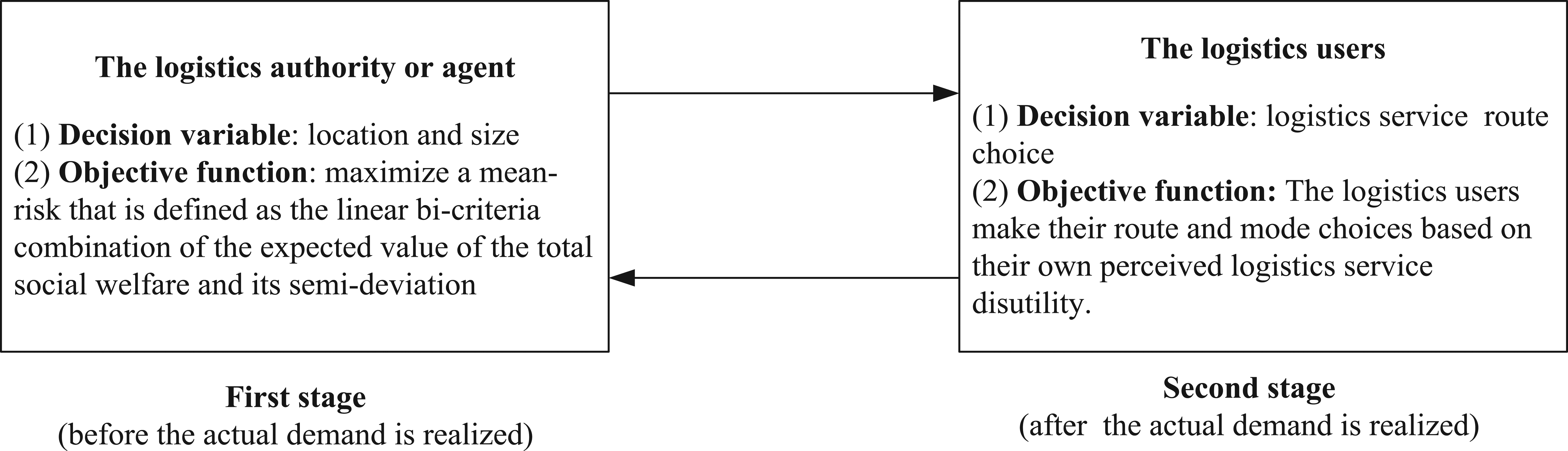
Framework of the two-stage decision model.

Scenario-based stochastic Logistics users’ service choice equilibrium

According to A3, the logistics users’ disutility consists of the logistics service time, transportation cost, and CO₂ emission taxes (if any), which can be expressed as

u_{w r}^{m s} = C_{w r}^{m s} + τ_{v o t} T_{w r}^{m s} + G_{w r}^{m s}, \forall r \in R_{w}, w \in W, m \in M, s \in Ω

(1)

where $C_{wr}^{ms}$ , $T_{wr}^{ms}$ , and $G_{wr}^{ms}$ represent the transportation cost, logistics service time, and CO₂ emission taxes on service route r by transport mode m between OD pair w under logistics demand scenario $s \in Ω$ , respectively. $τ_{vot}$ is the value of time (VOT).

The transportation cost and service time on a route can be expressed as the sum of the transportation costs and service times on all the transport arcs and transfer arcs (i.e. transfer nodes) along that route, including transfer cost and time, which are, respectively, expressed as

\begin{matrix} C_{wr}^{ms} = \sum_{a \in A^{g}} c_{a}^{m} l_{a} δ_{ar}^{m} + \sum_{i \in A^{t}} c_{i} δ_{ir}, \forall r \in R_{w}, \\ w \in W, m \in M, s \in Ω \end{matrix}

(2)

\begin{matrix} T_{wr}^{ms} = \sum_{a \in A^{g}} t_{a}^{ms} (v_{a}^{ms}) δ_{ar}^{m} + \sum_{i \in A^{t}} t_{i}^{s} δ_{ir}, \forall r \in R_{w}, \\ w \in W, m \in M, s \in Ω \end{matrix}

(3)

Considering the difference in the attributes of different transportation modes, the logistics service time on arc a for different modes should be estimated by different functions, as shown in equation (4). For the transportation mode of HGV or LGV, the Bureau of Public Roads (BPR) US type function can be used to estimate the service time.^13,41 For railway or waterway, the average transport service time and departure interval time should be considered, that is

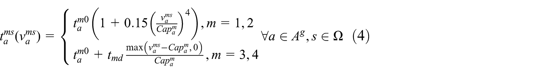
t_{a}^{ms} (v_{a}^{ms}) = {\begin{matrix} t_{a}^{m 0} (1 + 0.15 {(\frac{v_{a}^{ms}}{{Cap}_{a}^{m}})}^{4}), m = 1, 2 \\ t_{a}^{m 0} + t_{md} \frac{max (v_{a}^{ms} - {Cap}_{a}^{m}, 0)}{{Cap}_{a}^{m}}, m = 3, 4 \end{matrix} \forall a \in A^{g}, s \in Ω

(4)

where $t_{a}^{m 0}$ is the free-flow transport service time, and $t_{md}$ is the average shift interval for transport mode m.

The CO₂ emission taxes on route r between OD pair w can be expressed as the sum of the emission taxes on all the arcs along that route, that is

G_{wr}^{ms} = \sum_{a \in A^{g}} e^{m} l_{a} δ_{ar}^{m} z, \forall r \in R_{w}, w \in W, m \in M, s \in Ω

(5)

According to A3, the logistics service mode/route choices can be calculated by a logit-based stochastic user equilibrium (SUE) under logistics demand scenario. The flow $h_{wr}^{ms}$ on route r between OD pair $w \in W$ served by mode m can thus be given by

h_{w r}^{m s} = q_{w}^{s} \frac{\exp (- θ u_{w r}^{m s})}{\sum_{m \in M} \sum_{r \in R_{w}} \exp (- θ u_{w r}^{m s})}, \forall r \in R_{w}, w \in W, m \in M, s \in Ω

(6)

where the parameter $θ$ represents the variation of perception of logistics users on logistics service disutility. The higher the value of $θ$ , the smaller the variation in logistics users’ perception, and vice versa.^38,42,43

In order to capture the logistics users’ responses to logistics service disutility, an elastic travel demand function is introduced. It is assumed that the total resultant demand $q_{w}$ between OD pair $w$ is a continuous and monotonically decreasing function, $D_{w} (\cdot)$ , of the expected minimal service disutility $λ_{w}^{s}$ for the logistics OD pair concerned,⁴⁴ that is

q_{w}^{s} = D_{w} (λ_{w}^{s}), \forall w \in W, s \in Ω

(7)

In this article, we adopt the following demand function

q_{w}^{s} = {\bar{q}}_{w}^{s} \exp (- β λ_{w}^{s}), \forall w \in W, s \in Ω

(8)

where ${\bar{q}}_{w}^{s}$ is the potential logistics service demand between OD pair w, and $β$ is the demand dispersion parameter that reflects the demand sensitivity to the logistics service disutility by OD pair w under logistics demand scenario $s$ . According to random utility theory, $λ_{w}^{s}$ can be measured by the following log-sum formula shown in equation (9)^10,45

λ_{w}^{s} = - \frac{1}{θ} \ln (\sum_{m \in M} \sum_{r \in R_{w}} \exp (- θ u_{wr}^{ms}))

(9)

According to the theory of equilibrium network flow, the following constraints should be satisfied^44,46

\sum_{m \in M} q_{w}^{ms} = q_{w}^{s} \forall w \in W, s \in Ω

(10)

\sum_{r \in R_{w}} h_{wr}^{ms} = q_{w}^{ms} \forall w \in W, m \in M, s \in Ω

(11)

\sum_{m \in M} \sum_{w \in W} \sum_{r \in R_{w}} h_{wr}^{ms} δ_{ar}^{m} = v_{a}^{s} \forall a \in A, s \in Ω

(12)

\sum_{m \in M} \sum_{w \in W} \sum_{r \in R_{w}} h_{wr}^{ms} δ_{ir} = h_{i}^{s} \forall i \in A^{t}, s \in Ω

(13)

h_{wr}^{ms}, q_{w}^{ms}, q_{w}^{s} \geq 0, \forall w \in W, r \in R_{w}, m \in M, s \in Ω

(14)

where, equation (10) is the modal demand conservation constraint. Equation (11) is the route flow conservation constraint for the pure mode or combined mode. Equation (12) shows the relationship between the route flow and arc flow in the network. Equation (13) shows the relationship between the route flow and virtual arc flow (i.e. transferring flow) in the network. Equation (14) shows the non-negativity constraints for the route flows and OD pairs flow, respectively.

The network equilibrium for a multimodal logistics network with elastic demand with uncertain logistics demand can be defined as follows.

Definition 1

A network flow pattern $(h_{wr}^{s}, q_{w}^{ms}, q_{w}^{s})$ is a SUE for a multimodal logistics network with elastic demand and uncertain logistics demand if it satisfies equations (1)–(14).

Equivalent variational inequality model

The multimodal logistics network equilibrium conditions can be formulated as an equivalent variational inequality (VI) model.

Proposition 1

A flow pattern in a multimodal regional logistics network with elastic demand and uncertain logistics demand reaches the SUE state if and only if it satisfies the following VI condition

\begin{matrix} \sum_{w \in W} \sum_{r \in R} (U_{wr}^{ms} + \frac{1}{θ} \ln \frac{h_{wr}^{ms *}}{q_{w}^{ms *}}) (h_{wr}^{ms} - h_{wr}^{ms *}) \\ + \sum_{w \in W} \frac{1}{θ} \ln \frac{q_{w}^{sm *}}{q_{w}^{s *}} (q_{w}^{ms} - q_{w}^{ms *}) - \sum_{w \in W} \frac{1}{β} \ln \frac{q_{w}^{s *}}{{\bar{q}}_{w}^{s}} (q_{w}^{s} - q_{w}^{s *}) \geq 0 \end{matrix}

(15)

\sum_{m \in M} q_{w}^{ms} = q_{w}^{s} \forall w \in W, s \in Ω

(16)

\sum_{r \in R_{w}} h_{wr}^{ms} = q_{w}^{ms} \forall w \in W, m \in M, s \in Ω

(17)

\sum_{m \in M} \sum_{w \in W} \sum_{r \in R_{w}} h_{wr}^{ms} δ_{ar}^{m} = v_{a}^{s} \forall a \in A, s \in Ω

(18)

\sum_{m \in M} \sum_{w \in W} \sum_{r \in R_{w}} h_{wr}^{ms} δ_{ir} = h_{i}^{s} \forall i \in A^{t}, s \in Ω

(19)

h_{wr}^{ms}, q_{w}^{ms}, q_{w}^{s} \geq 0, \forall w \in W, r \in R_{w}, m \in M, s \in Ω

(20)

where $Γ$ is the feasible set of the network flow pattern under uncertain logistics demand $(h_{wr}^{ms}, q_{w}^{ms}, q_{w}^{s})$ , satisfying the constraints (16)–(20). In inequality (15), $(h_{wr}^{ms *}, q_{w}^{ms *}, q_{w}^{s *})$ represents the optimal solution to the VI model, and $U_{wr}^{ms}$ is the corresponding logistics disutility value computed at the optimal solution point $(h_{wr}^{ms *}, q_{w}^{ms *}, q_{w}^{s *})$ . The proof of Proposition 1 is given in Appendix 2.

Robust design problem for the sustainable regional logistics networks design

As stated in section “Introduction,” the traditional expectation model may lead to a large variation in the logistics system performance for different logistics demand scenarios. In order to hedge against the instability of the model solution due to the future logistics demand uncertainty, a robust risk-averse objective function and some chance constraints are introduced as follows.

Chance constraints

Chance constraint of link capacity.

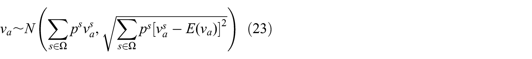
Since the future logistics demand in the regional logistics system is a random variable, the flow over logistics arcs, which depends on the actual logistics demand, is also stochastic. Let $p^{s}$ be the probability of scenario s. The expected value $E (v_{a})$ and the standard deviation $D (v_{a})$ of flow on arc $v_{a}$ are then given by

E (v_{a}) = \sum_{s \in Ω} p^{s} v_{a}^{s} \begin{matrix} \forall a \in A \end{matrix}

(21)

D (v_{a}) = \sqrt{\sum_{s \in Ω} p^{s} [v_{a}^{s} - E (v_{a})]^{2}} \begin{matrix} , \forall a \in A \end{matrix}

(22)

From equation (12), the arc flow can be expressed as the sum of the flows of logistics service routes traversing that arc (i.e. $\sum_{m \in M} \sum_{w \in W} \sum_{r \in R_{w}} h_{wr}^{ms} δ_{ar}^{m} = v_{a}^{s}$ ). For simplicity, we assume that the route flows are independently distributed random variables, as assumed in Clark and Watling.⁴⁷ According to the central limit theorem, as long as the Lindeberg’s condition is satisfied, the link flow follows a normal distribution regardless of the route flow distribution. For the details of the proof, readers can refer to Lo and colleagues.^48–50 Therefore, the arc flow $v_{a}$ distribution can be expressed as normal distribution as follows

v_{a} ~ N (\sum_{s \in Ω} p^{s} v_{a}^{s}, \sqrt{\sum_{s \in Ω} p^{s} [v_{a}^{s} - E (v_{a})]^{2}})

(23)

The chance constraint of the arc capacity requires that the flow on each arc does not exceed the capacity of that arc with a certain probability or confidence level $α_{c}$ represented as

p {v_{a} \leq C_{a}^{0}} \geq α_{c} or p {\frac{v_{a} - E (v_{a})}{D (v_{a})} \leq \frac{C_{a}^{0} - E (v_{a})}{D (v_{a})}} \geq α_{c}

(24)

The above equation can be further written as

E (v_{a}) + Φ^{- 1} (α_{c}) D (v_{a}) \leq C_{a}^{0} \begin{matrix} \forall a \in A \end{matrix}

(25)

where $Φ^{- 1} (\cdot)$ is the inverse cumulative distribution function of standard normal distribution.

2. Chance constraint of environmental tolerance.

Environmental sustainability, as an important component of sustainable urban development, requires that the vehicular emissions on each arc of the network do not exceed a given threshold with a certain confidence level. Let $e_{a}^{s}$ be the total amount of transport emissions on arc a under scenario s. The total amount of traffic emissions on arc $a$ can be defined as the product of the flow on arc a and an emission factor, that is

W_{a}^{s} = \sum_{m} v_{a}^{ms} l_{a}^{m} e_{a}^{m} \begin{matrix} \forall a \in A \end{matrix}, s \in Ω

(26)

where $e_{a}^{m}$ is the CO₂ emission factor of transport tool $m$ over arc $a$ , which is assumed to be a constant.

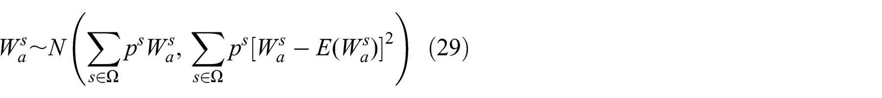
Obviously, the amount of CO₂ emissions over arc $a$ , $W_{a}^{s}$ , is a random variable. Its expected value $E (W_{a}^{s})$ and standard deviation $D (W_{a}^{s})$ , respectively, are given by

E (W_{a}^{s}) = \sum_{s \in Ω} p^{s} W_{a}^{s} \begin{matrix} \forall a \in A \end{matrix}

(27)

D (W_{a}^{s}) = \sqrt{\sum_{s \in Ω} p^{s} [W_{a}^{s} - E (W_{a}^{s})]^{2}} \begin{matrix} , \forall a \in A \end{matrix}

(28)

From equation (26), the amount of CO₂ emissions on an arc is a linear function of the flow on that arc. Thus, it also follows a normal distribution, that is

W_{a}^{s} ~ N (\sum_{s \in Ω} p^{s} W_{a}^{s}, \sum_{s \in Ω} p^{s} [W_{a}^{s} - E (W_{a}^{s})]^{2})

(29)

The chance constraint of the environmental tolerance can then be obtained as

E (W_{a}^{s}) + Φ^{- 1} (α_{w}) D (W_{a}^{s}) \leq W_{a}^{0} \begin{matrix} \forall a \in A \end{matrix}

(30)

where $W_{a}^{0}$ is the threshold of the environmental tolerance and $α_{w}$ is the confidence level. Equation (30) means that the actual total emissions on arc a does not exceed that of environmental threshold with a certain probability or confidence level $α_{w}$ .

Model formulation of the robust regional logistics design problem

We define the total social welfare under scenario $s$ as follows

\begin{matrix} Z^{s} (X, Y) = (\sum_{w \in W} \int_{0}^{q_{w}^{s}} D_{w}^{- 1} (w) dw - \sum_{w \in W} q_{w}^{s} λ_{w}^{s}) \\ + (\sum_{i \in I} C_{i} h_{i}^{s} - \sum_{i \in I} C_{i}^{0} {(y_{i})}^{ρ} x_{i} - \sum_{i \in I} η_{i} h_{i}^{s}) \\ + (\sum_{m \in M} \sum_{a \in A} v_{a}^{ms} c_{a}^{m} - \sum_{m \in M} \sum_{a \in A} v_{a}^{ms} τ_{a}^{m} + \sum_{m \in M} \sum_{a \in A} v_{a}^{ms} l_{a} e_{a}^{m} z) \end{matrix}

(31)

s . t . x_{i} = {0, 1}, \forall i \in P

(32)

s_{i}^{min} \leq y_{i} \leq s_{i}^{max}, \begin{matrix} \forall i \in P \end{matrix}

(33)

\sum_{i \in I} C_{i}^{0} {(y_{i})}^{ρ} x_{i} \leq B

(34)

where $(X, Y)$ is the vector of the decision variables: location and size of logistics parks.

The objective function (31) includes three components: the first bracket represents consumer surplus (denoted as CS), whereas the sum of the second term (i.e. the revenue at logistics nodes) and the third term (i.e. the revenue of logistics services on arcs) is the producer surplus. $D_{w}^{- 1} (\cdot)$ is the inverse function of the logistics demand function. Constraint (32) expresses a binary variable with regard to the location of a logistics park, where “1” represents the decision to construct a logistics park at node i, and 0 otherwise. Constraint (33) represents the constraint of sizes for candidate logistics park i. Constraint (34) implies that the investment of logistics parks satisfies the total capital budget.

The total social welfare of logistics system, defined in equation (31), is a random variable, and its expected value E(Z) can be expressed as

E (Z^{s} (X, Y)) = \sum_{s \in Ω} p^{s} Z^{s} (X, Y)

(35)

We now introduce the semi-deviation as a measure of solution robustness, as in Ahmed⁵¹ and Santoso et al.,⁵² which is defined as

Θ (Z^{s}) = E [Z^{s} - E (Z^{s})]_{+} = \sum_{s \in Ω} p^{s} [Z^{s} - \sum_{s \in Ω} p^{s} Z^{s}]_{+}

(36)

where $[x]_{+} = max {0, x}$

The semi-deviation, but not the variance (or standard deviation), is used as an indicator for the risk measure because variance is a symmetric statistic and gives equal weight to deviations above and below the mean without addressing the risks associated with extreme outcomes,^39,53,54 and because mean-variance does not preserve the convexity of the objective function.⁵¹ The semi-deviation risk measure defined in equation (37) overcomes these shortcomings.

In view of the above, the robust risk-averse regional logistics network design model can be formulated as given below

\begin{matrix} max φ (X, Y) = E (Z^{s}) - λ Θ (Z^{s}) \\ = \sum_{s \in Ω} p^{s} Z^{s} (X, Y) - λ \sum_{s \in Ω} p^{s} [Z^{s} - \sum_{s \in Ω} p^{s} Z^{s}]_{+} \end{matrix}

(37)

Subject to

E (v_{a}) + Φ^{- 1} (α_{c}) D (v_{a}) \leq C_{a}^{0} \begin{matrix} \forall a \in A \end{matrix}

(38)

E (W_{a}^{s}) + Φ^{- 1} (α_{w}) D (W_{a}^{s}) \leq W_{a}^{0} \begin{matrix} \forall a \in A \end{matrix}

(39)

x_{i} = {0, 1}, \forall i \in P

(40)

s_{i}^{min} \leq y_{i} \leq s_{i}^{max}, \begin{matrix} \forall i \in P \end{matrix}

(41)

\sum_{i \in I} C_{i}^{0} {(y_{i})}^{ρ} x_{i} \leq B

(42)

where $(v_{a}^{s}, h_{wr}^{ms}, q_{w}^{ms}, q_{w}^{s})$ can be calculated by solving the scenario-based stochastic logistics service route choice equilibrium problem (15)–(20). In this model, $λ$ is a non-negative weighting factor that reflects the significance of the risk measure for the objective function. Constraint (40) expresses a binary variable with regard to the location of a logistics park, where “1” represents the decision to construct a logistics park at node i, and 0 otherwise. Constraint (41) represents the size limitation of logistics park i, where $s_{i}^{min}$ and $s_{i}^{max}$ are the lower and upper bounds of candidate logistics parks, respectively. Constraint (42) indicates that the total budge should be satisfied.

Solution algorithm

In this section, the sample average approximation (SAA) scheme is used to approximate the robust optimization problem (37)–(42). The penalty function method is embedded by GA which is developed to solve the approximate problem.

SAA-based scheme

In the SAA-based scheme, we generate a sample of size $N$ , or ${s_{1}, s_{2}, s_{3}, \dots, s_{k}, \dots, s_{N}}$ , for the stochastic distribution of the logistics demand. The robust model (37)–(42) can then be approximated by the following SAA model

max φ_{N} (X, Y) = \frac{1}{N} \sum_{k = 1}^{N} Z^{s_{k}} - \frac{λ}{N} \sum_{k = 1}^{N} {[Z^{s_{k}} - \frac{1}{N} \sum_{k = 1}^{N} Z^{s_{k}}]}_{+}

(43)

Subject to

\frac{1}{N} \sum_{k = 1}^{N} v_{a}^{s_{k}} + Φ^{- 1} (α_{c}) \sqrt{\sum_{k = 1}^{N} [\frac{1}{N} {(v_{a}^{s_{k}} - \frac{1}{N} \sum_{k = 1}^{N} v_{a}^{s_{k}})}^{2}]} \leq C_{a}^{0}

(44)

\begin{matrix} \frac{1}{N} \sum_{k = 1}^{N} W_{a}^{s_{k}} + Φ^{- 1} (α_{w}) \\ \sqrt{\sum_{k = 1}^{N} [\frac{1}{N} {(W_{a}^{s_{k}} - \frac{1}{N} \sum_{k = 1}^{N} W_{a}^{s_{k}})}^{2}]} \leq W_{a}^{0} \end{matrix}

(45)

x_{i} = {0, 1}, \forall i \in P

(46)

s_{i}^{min} \leq y_{i} \leq s_{i}^{max}, \begin{matrix} \forall i \in P \end{matrix}

(47)

\sum_{i \in I} C_{i}^{0} {(y_{i})}^{ρ} x_{i} \leq B

(48)

where $(v_{a}^{s}, h_{wr}^{ms}, q_{w}^{ms}, q_{w}^{s})$ can be calculated by solving the scenario-based stochastic logistics service route choice equilibrium problem (15)–(20).

Penalty function approach embedded by a GA

Note that there are side constraints (44)–(45) in the approximate problem (38)–(42). These side constraints can be incorporated into the objective function (43) using the penalty function approach, that is

{\hat{φ}}_{N} (X, Y) = φ_{N} (X, Y) - ζ Λ_{N} (X, Y)

(49)

where $ζ$ is the penalty multiplier, and

\begin{matrix} Λ_{N} (X, Y) = \sum_{a \in A} max {0, \frac{1}{N} \sum_{k = 1}^{N} v_{a}^{s_{k}} + Φ^{- 1} (α_{c}) \sqrt{\sum_{k = 1}^{N} [\frac{1}{N} {(v_{a}^{s_{k}} - \frac{1}{N} \sum_{k = 1}^{N} v_{a}^{s_{k}})}^{2}]} - C_{a}^{0}} \\ + \sum_{a \in A} max {0, \frac{1}{N} \sum_{k = 1}^{N} W_{a}^{s_{k}} + Φ^{- 1} (α_{w}) \sqrt{\sum_{k = 1}^{N} [\frac{1}{N} {(W_{a}^{s_{k}} - \frac{1}{N} \sum_{k = 1}^{N} W_{a}^{s_{k}})}^{2}]} - W_{a}^{0}} \end{matrix}

(50)

Accordingly, models (38)–(42) can further be written as

max {\hat{φ}}_{N} (X, Y) = φ_{N} (X, Y) - ζ Λ_{N} (X, Y)

(51)

where $(v_{a}^{s}, h_{wr}^{ms}, q_{w}^{ms}, q_{w}^{s})$ can be calculated by solving the scenario-based stochastic logistics service route choice equilibrium problem (15)–(20).

The above model can then be solved using the GA based on penalty function approach. The step-by-step procedure of the GA in conjunction with the penalty function approach is given as follows.

Solving the logistics authority robust risk-averse decision problem—first-stage problem (Algorithm 1).

Step 0. Initialization. Generate a sample of size N for logistics demand OD1 and OD2, that is, N logistics demand scenarios ${s_{1}, s_{2}, s_{3}, \dots, s_{k}, \dots, s_{N}}$ .

Step 1. Outer loop operation (solve the first-stage problem—logistics authority decision loop). Using GA to solve the first-stage problem (58).

Step 2. GA initialization.

(a) Set the GA parameters: the probability of crossover (Pc) and the probability of mutation (Pm).

(b) Set a stopping tolerance $ε_{1}$ and $ε_{2}$ , an initial penalty multiplier $ζ_{0}$ and a scale parameter $ω > 1$ .

(c) Set n = 0, and create the initial population pop_n = ${G_{k}^{n} | k = 1, 2, \dots, p}$ , in which individual $G_{k}^{n}$ is the kth decision scheme in the nth generation $p$ in the population size, where $G_{k}^{n} = {X_{k}^{n}, Y_{k}^{n})$ .

Step 3. Inner loop operation (solve the second-stage problem—logistics service route flow assignment).

For each logistics demand scenario $s_{i}$ , applying the following Algorithm 2 to solve the scenario-based SUE problem (1)–(14) for a given logistics authority decision $G_{k}^{n} = {X_{k}^{n}, Y_{k}^{n})$ , and obtain $h^{s_{i}, (n)} = (h_{wr}^{s_{i}, m (n)}, q_{w}^{s_{i}, m (n)}, q_{w}^{s_{i}, (n)})$ .

Step 4. Compute the objective function value ${\hat{φ}}_{N} (X_{k}^{(n)}, Y_{k}^{(n)})$ according to equations (49)–(51) for all individual $G_{k}^{n}$ .

Step 5. Calculate the fitness value of $G_{k}^{n}$ .

For each $G_{k}^{n}$ of pop_n , calculate the fitness value ${fit}_{k}^{n}$ and $G_{k}^{n}$ based on ${\hat{φ}}_{N} (X_{k}^{(n)}, Y_{k}^{(n)})$ .

Step 6. Sort the individual $G_{k}^{n}$ of the population $po p_{n}$ in descending order according to the value ${fit}_{k}^{n}$ .

Step 7. Implement selection, crossover, and mutation

Implement selection, crossover, and mutation according to ${fit}_{k}^{n}$ and finally obtain a new population $po p_{n}$ and n = n + 1 go to Step 2.

Step 8. Termination check for the outer loop operation.

If $ζ_{n} Λ_{N} (X_{k}^{(n)}, Y_{k}^{(n)}) \leq ε_{1}$ and ${\hat{φ}}_{N} (X_{k}^{(n)}, Y_{k}^{(n)}) - {\hat{φ}}_{N} (X_{k}^{(n - 1)}, Y_{k}^{(n - 1)}) \leq ε_{2}$ ( $ε_{1}$ and $ε_{2}$ are the two pre-specified precision parameters), then stop the calculation; otherwise, set $ζ_{n + 1} = ω ζ_{n}$ , $n = n + 1$ go to Step 2.

Step 9. Output the optimal result.

The flow chart of Algorithm 1 is shown in Figure 4(a).

2. Solving the logistics service routing choice equilibrium problem by the Gauss–Seidel decomposition approach—second-stage problem (Algorithm 2).

Step 1. Initialization. Set iteration index n = 1. Let $v_{a}^{(0)} = 0, \forall a \in A$ and set the logistics service time and fare under the free-flow conditions for all arcs, compute the route logistics service cost, time, and CO₂ emission taxes ${C_{wr}^{m}, T_{wr}^{m}, G_{wr}^{m}, \forall r \in R_{w}, w \in W, m \in M}$ according to equations (2), (3), and (5).

Step 2. Calculating the disutility. Calculate the disutility of all logistics service routes $u_{wr}^{m}$ according to equation (1). Compute the expected minimum disutility, $λ_{w}$ , between logistics OD pair w based on equation (9).

Step 3. Calculating logistics demand. Calculate the resultant demand for each OD pair w based on equation (8).

Step 4. Computing the logistics service demand, mode share, and transfer flows. Use equations (8), (10), (11), and (13) to compute $q_{w}^{(n)}$ and $q_{w}^{m (n)}$ , respectively.

Step 5. Logit-based SUE assignment. Conduct logit-based SUE assignment to get auxiliary arc flow $g_{a}^{(n)}, a \in A$ based on equation (12).

Step 6. Method of successive average. Let $v_{a}^{(n + 1)} = v_{a}^{(n)} + (1 / (n + 1)) (g_{a}^{(n)} - v_{a}^{(n)}), a \in A$ .

Step 7. Convergence check. Define $gap (n) = \frac{\sqrt{\sum_{a \in A} {(v_{a}^{(n + 1)} - v_{a}^{(n)})}^{2}}}{\sum_{a \in A} v_{a}^{(n)}}$ , if $gap (n) \leq ξ$ , then go to Step 9 and output all results as the final solution, where $ξ$ is a predetermined parameter.

Step 8. Set n = n + 1. Compute all arc transport costs and route transport costs on the basis of current arc flows, then go to Step 2.

Step 9. Output the resultant demand and corresponding network flow pattern $h = (h_{wr}^{m}, q_{w}^{m}, q_{w})$ .

The flow chart of Algorithm 2 is shown in Figure 4(b).

Figure 4.

Flow chart of (a) Algorithm 1 and (b) Algorithm 2.

Key elements design of GA

In this section, we explain three key elements of the GA: the coding, selection, crossover, and mutation methods.

Coding method

The chromosome of the individual in the GA is made up of two parts as shown in Figure 5.

Figure 5.

Chromosome of the GA.

Part 1 represents whether the candidate logistics park is open, the value is 1 when the candidate logistics park is open and 0 otherwise. As shown in Part 2, if the candidate logistics park is open, which size can been used a random positive real number r in $[s_{i}^{min} s_{i}^{max}]$ .

Selection method

The selection process is applied with the method of spinning the roulette wheel selection operator. We can adopt the so-called rank-based evaluation function as follows

Eval (V_{i}) = a {(1 - a)}^{i - 1}, \forall i = 1, 2, 3, \dots, pop_size .

We mention that i = 1 means the best individual, while $i = pop_size$ means the worst individual, and of course $\sum_{i = 1}^{pop_size} Eval (V_{i}) \approx 1$ .

The selection process is based on spinning the roulette wheel pop_size times, each time selecting a single chromosome for a new population in the following way:

Step 1. Calculate the cumulative probability $Cum (i)$ for each chromosome $V_{i}$ , $Cum (0) = 0$

Cum (i) = \sum_{j = 1}^{i} Eval (V_{j}), i = 1, 2, 3, \dots, pop_size

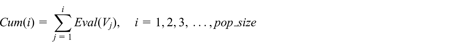
Step 2. Generate a random real number $r$ in $(0, Cum (i)]$ .

Step 3. Select the ith chromosome $V_{i} (1 \leq i \leq pop_size)$ such that $Cum (i - 1) < r \leq Cum (i)$ .

Step 4. Repeat Steps 2 and 3 pop_size times and obtain pop_size copies of chromosomes.

Crossover and mutation method

Crossover operator.

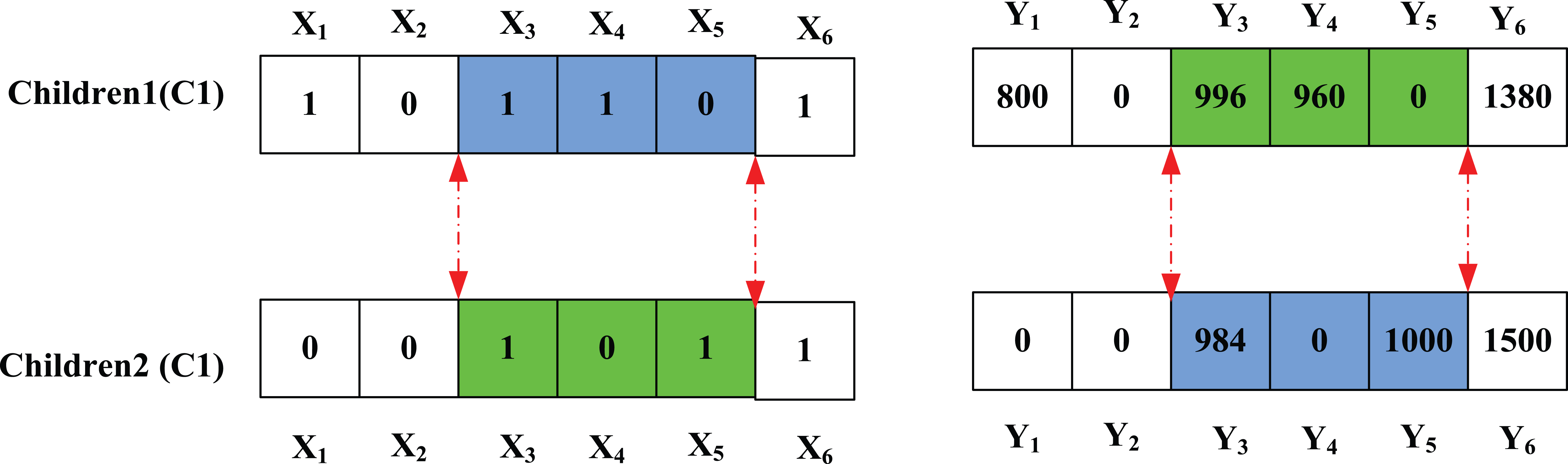
We implement a crossover operation for the two parts of the chromosome. The two-point crossover method is adopted for Part 1. The crossover operation of Part 2 is a convex combination of two corresponding parents. For each pair of parents (vectors Y ₁ and Y ₂), the size crossover operator on Y _l and Y ₂ will produce two children C ₁ and C ₂ as follows

C_{1}^{i} = λ_{1} Y_{i}^{1} + λ_{2} Y_{i}^{2}

C_{2}^{i} = λ_{2} Y_{i}^{1} + λ_{1} Y_{i}^{2}

where $λ_{1}, λ_{2} > 0; λ_{1} + λ_{2} = 1$ .

We give a simple example as follows, which consists of six candidate logistics parks as shown in Figure 6. Let V₁ and V₂ denote the chromosomes of parent1 and parent2 respectively. And Let C₁ and C₂ denote the corresponding chromosomes of the child1 and child2 after crossover operator respectively. The parameters of crossover operation of Part 2 are set to $λ_{1} = 0.2; λ_{2} = 0.8$ .

Figure 6.

Representation of the crossover operation.

It is possible that the crossover operation produces certain “problem chromosomes,” which describes an unfeasible logistics park design scheme. For example, it is to obtain a problem chromosome as shown in Figure 6(b). Here, the value of $X_{5}$ in Part1 of child 1 (C ₁) is 0, but the corresponding size $(Y_{i})$ of Part 2 is 250. So, this is an unfeasible location scheme. As shown in Figure 7, the problem chromosomes can be corrected by the following rules: (1) if the value of $X_{i}$ is 0 and the corresponding value of $Y_{i}$ is set to 0; (2) if the value of $X_{i}$ is 1 and the value of $Y_{i}$ does not fall in the interval $[s_{i}^{min}, s_{i}^{max}]$ , the latter should be set as a random positive real number r in $[s_{i}^{min} s_{i}^{max}]$ .

Figure 7.

Children chromosome after correcting.

Mutation operator.

Generating a random real number r in [0, 1], we select the given chromosome for mutation.

If r < Pm. Let a parent for mutation $V$ , denoted by a vector $V = (X, Y)$ , be selected. For the first part (i.e. vector X), the two-point mutation method is adopted, which is shown in Figure 8. For the second part (i.e. vector Y), we use the $Y + M \cdot d$ to replace the $Y$ . If the vector $Y + M \cdot d$ is not feasible for the inequality constraints, then we set $M$ as a random number between 0 and $M$ until it is feasible. If the above process cannot find a feasible solution in a predetermined number of iterations, we take $M = 0$ . Thus the offspring is $Y' = Y + M \cdot d$ .

Figure 8.

Representation of the mutation operation.

Illustrative numerical example

To facilitate the presentation of the essential ideas and contributions of this article, the proposed model and the solution algorithm are applied to a simple logistics service network. In this section, the solutions for different types of optimization models are compared to show the importance of the consideration of logistics demand uncertainty and risk for low-carbon logistics network design. Sensitivity analysis to some key model parameters, such as the CV of total logistics demand, risk-averse parameter, and confidence levels of chance constraints, is also carried out for providing some insightful findings.

Problem setting

In the following, a numerical example is used to illustrate the applications of the proposed model and solution algorithm. The example regional logistics network is shown in Figure 9. It consists of two logistics demand OD pairs, that is, OD pair 1 (1 → 8) and OD pair 2 (1 → 7), 8 nodes and 15 links which are denoted by arc i (i = 1, 2, 3, …, 15). In this figure, nodes 3, 4, and 5 are assumed to be three candidate logistics parks.

Figure 9.

Original logistics service network.

Figures 9 and 10 show the original and modified logistics service networks, respectively. For some links, different vehicle types are available, and one link that is served by different vehicle types can thus be expanded as different links. For example, link 1 in the original logistics service network (i.e. Figure 9) can be expanded as arcs 1 and 16, as shown in the modified logistics service network (i.e. Figure 10). The basic data for the logistics service network are given in Table 1.

Figure 10.

Modified logistics service network.

Table 1.

Basic input data for the logistics service network.

Arc	Mode	Length (km)	Free-flow travel speed time (km/h)	Capacity of CO₂ emissions (kg/week)	Capacity of arc (tons/week)	Transport cost per unit of shipment ($/ton km)
1	HGV	800	60	150,000	800	0.4
2	HGV	1200	60	200,000	800	0.4
3	Railway	1000	50	100,000	1200	0.3
4	Waterway	1200	30	80,000	1500	0.2
5	Waterway	300	30	80,000	1200	0.2
6	HGV	400	60	150,000	1000	0.4
7	HGV	350	60	150,000	1000	0.4
8	Railway	300	50	100,000	1200	0.3
9	HGV	500	60	250,000	400	0.4
10	HGV	550	60	200,000	400	0.4
11	HGV	80	60	200,000	400	0.42
12	LGV	50	45	120,000	900	0.42
13	HGV	80	60	100,000	400	0.42
14	LGV	60	45	120,000	500	0.42
15	LGV	40	45	100,000	600	0.42
16	LGV	800	60	100,000	400	0.41
17	LGV	1200	60	150,000	400	0.41
18	LGV	500	60	150,000	400	0.41
19	LGV	550	60	100,000	400	0.41
20	LGV	80	60	200,000	400	0.42
21	LGV	50	45	120,000	900	0.42
22	LGV	80	60	100,000	400	0.42
23	LGV	60	45	120,000	500	0.42
24	LGV	40	45	100,000	600	0.42

HGV: heavy goods vehicle; LGV: light goods vehicle.

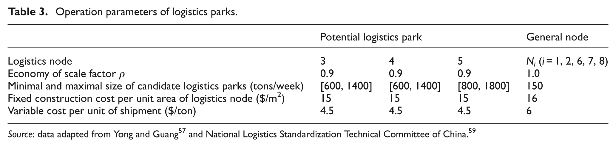
Suppose that the logistics OD pair 1 (from node 1 to node 8) serves agricultural goods, in which potential demand follows a normal distribution $Q_{1} ~ N (1000, {(100)}^{2})$ units per week, whereas the logistics OD pair 2 (from node 1 to node 7) serves industrial goods with a normal distribution potential demand $Q_{2} ~ N (1200, {(100)}^{2})$ .The sample size of logistics demand scenarios is 300. The risk-averse parameter $λ$ is set to be 10. The total capital budget available is B = 16,500$. The parameters $θ$ and $β$ are 0.0006 and 0.02, respectively. The VOT is $10 per hour.^55,56 The transfer cost and time at the logistics transfer node are shown in Table 2.^57,58 The other parameters are shown in Table 3.^57,59 The average emissions of different transportation modes are different. Specifically, the average emissions of HGV, LGV, railway, and waterway are 0.132, 0.283, 0.022, and 0.016 (kg/ton km), respectively.^58,60 The parameter z on CO₂ emission taxes is 0.09 $/kg. The confidence levels for the chance constraints are $α_{c} = α_{w} = 95 %$ . After many trial-and-error experiments, the following parameters for the penalty function and GA are chosen: $ζ = 2$ , $P_{c} = 0.5$ , $P_{m} = 0.2$ , and $pop_size = 30$ . In the following analyses, unless specified otherwise, the input data above are considered as the reference or base case.

Table 2.

Transfer time and cost at the general logistics nodes.

Mode	HGV	LGV	Railway	Waterway
HGV	0 (0)	1.5 (5)	4 (12)	2 (14)
LGV	1.5 (5)	0 (0)	3 (11)	1.5 (13)
Railway	1.5 (12)	3 (11)	0 (0)	4 (9)
Waterway	2 (14)	1.5 (13)	4 (9)	0 (0)

HGV: heavy goods vehicle; LGV: light goods vehicle.

Numbers inside and outside the brackets are transfer cost ($/ton) and transfer time (h), respectively.

Source: data adapted from Qu et al.¹ and Yong and Guang.⁵⁷

Table 3.

Operation parameters of logistics parks.

	Potential logistics park			General node
Logistics node	3	4	5	N_i (i = 1, 2, 6, 7, 8)
Economy of scale factor ρ	0.9	0.9	0.9	1.0
Minimal and maximal size of candidate logistics parks (tons/week)	[600, 1400]	[600, 1400]	[800, 1800]	150
Fixed construction cost per unit area of logistics node ($/m²)	15	15	15	16
Variable cost per unit of shipment ($/ton)	4.5	4.5	4.5	6

Source: data adapted from Yong and Guang⁵⁷ and National Logistics Standardization Technical Committee of China.⁵⁹

Numerical results and discussions

Applying the proposed model and solution algorithm to the example network, the results are summarized as follows.

We first investigate the performance and convergence of the proposed solution algorithms. The proposed solution algorithm was coded in Microsoft Visual C++ 6 and run on a laptop Dell N5040 with an Intel Pentium 2.13-GHz CPU and 4.00 GB RAM. And the iterative process for the reference case takes about 1978.44 s of CPU time. Figure 11 shows the convergent of situations of GA method for solving the first-stage problem. It shows that the value of the total social welfare increases quickly with the number of iterations and then tends to stabilize after about 50 iterations.

Figure 11.

Convergence of genetic algorithm (GA).

Table 4 indicates the optimal solutions and associated system performances for three different models, including the robust model, expectation model, and deterministic model. The expectation model refers to optimize the exact value of the objective without considering the risk of variation of logistics demand, which means the risk-averse parameter $λ$ in equation (37) is 0, while the deterministic model refers to the logistics demand is fixed, that is, the value of CV on total logistics demand is 0.

Table 4.

Comparison of solutions of the robust, expectation, and deterministic models.

Model type	Robust model	Expectation model	Deterministic model
Expected system utility ($/week)	2,198,322	2,194,686	2,221,212
Location decision	Nodes 5 and 6	Nodes 5 and 6	Nodes 5 and 6
Size decision (m²)	832, 1116	845, 1199	886, 1208

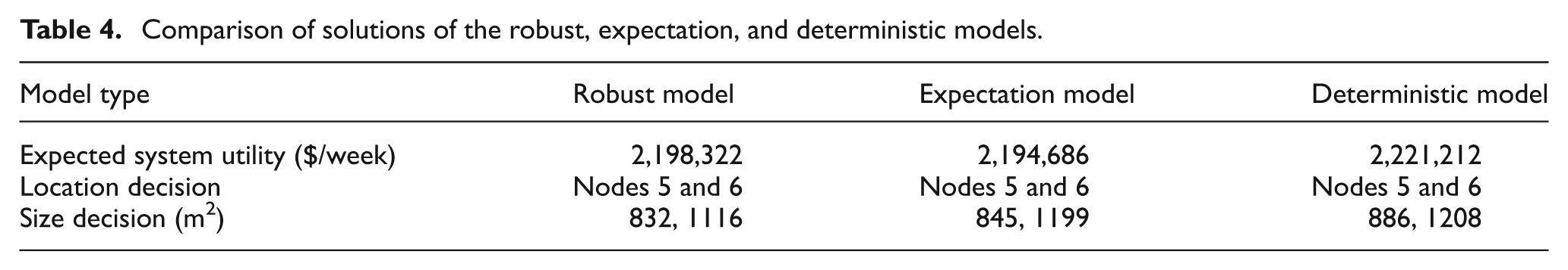
It shows that the expected total social welfare of the robust model is the lowest (2,198,322 $/week), that of the deterministic model is the highest (2,221,212 $/week), and that of the expectation model is in between (2,194,686 $/week). This means that ignoring the effects of the demand uncertainty may lead to an overestimation of the expected total social welfare.

Figure 12 depicts the expected total social welfare for different budget levels for the robust model and the expectation model when the CV of logistics demand uncertainty is fixed at 0.1 and the confidence levels of all the chance constraints are fixed at 95%. It can be seen that the total social welfare quickly increases for low-budget levels for these two models, and then tends to stabilize when the budget level reaches 17,000$ (i.e. the critical level). This is because the budget constraint becomes inactive (or unbinding) after the critical level. In addition, for a given budget level, the expected total social welfare under the expected model is always higher than that under the robust model, and the difference between them enlarges with the budget level before reaching the critical level.

Figure 12.

Expected total social welfare against budget levels for robust and expectation models.

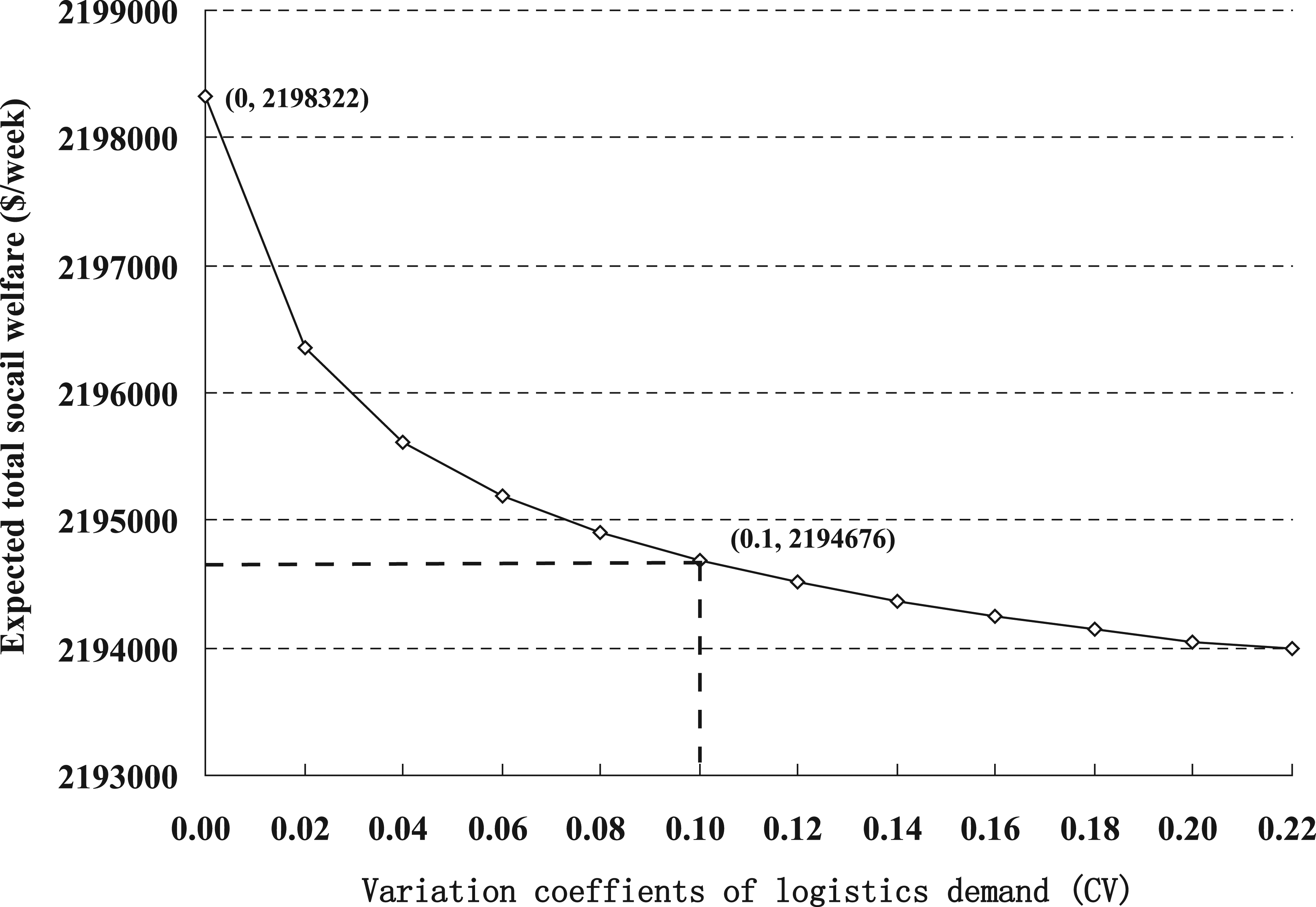
To examine the effects of the logistics demand uncertainty and risk measure, as shown in Figure 13, we can find that for a fixed value of risk-averse parameter, for example, $λ = 10$ as the CV increases from 0 (i.e. deterministic model) to 0.22 (i.e. stochastic model), the expected system utility decreases from 2,198,322 to 2,193,990 $/week. This implies that a lager value of CV leads to more variable (or unstable) total social welfare.

Figure 13.

Expected total social welfare against variation confident parameter (CV).

Figure 14 shows the expected total social welfare for different values of risk-averse parameter λ. It can be observed that for a fixed CV (e.g. CV = 0.1), as the risk-averse parameter increases from 0 (i.e. expectation model) to 15 (i.e. robust model), the expected total social welfare decreases from 2,198,322 to 2,194,433 $/week. This means that a lager value leads to more robust system performance but a lower expected total social welfare, and vice versa. Therefore, ignoring the risk term may lead to an overestimation of the expected total social welfare. In a robust region green logistics network design, a trade-off should be made between the expected system performance and its risk.

Figure 14.

Expected total social welfare against risk-averse parameter (λ).

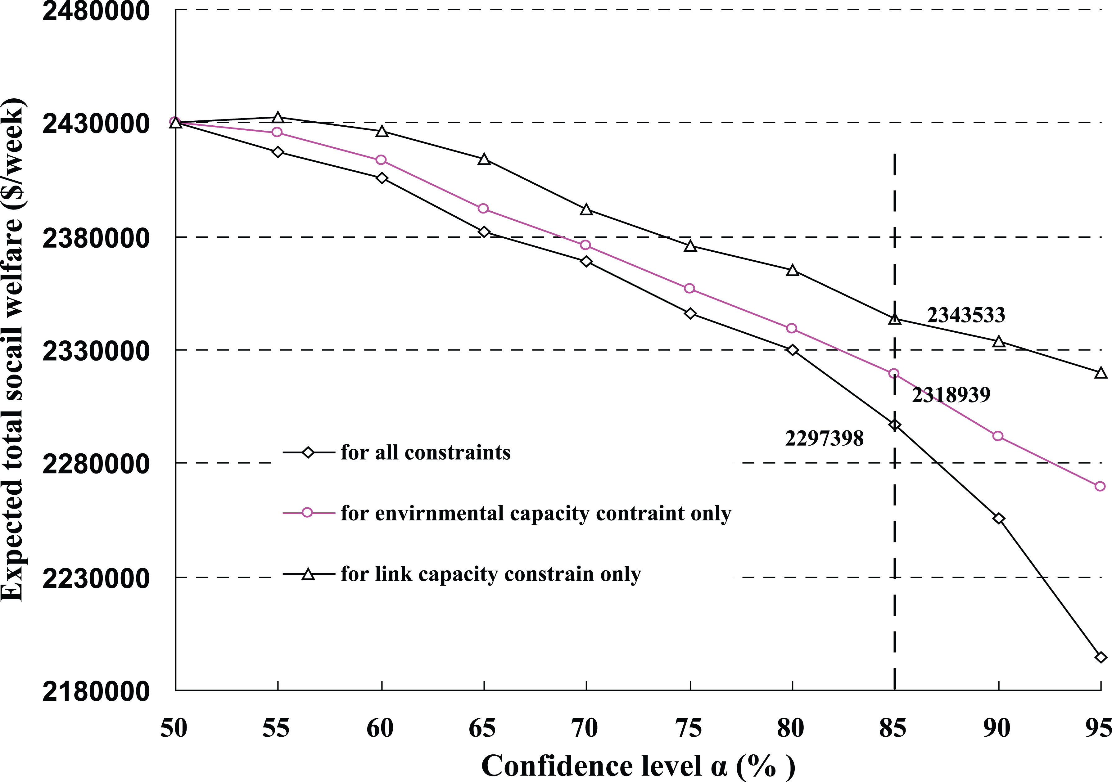
Finally, we examine the effects of the confidence levels of various chance constraints as shown in Figure 15. Three cases are considered, namely, Case 1: changing the confidence levels of all the chance constraints; Case 2: changing the confidence level of the link capacity chance constraint only (equation (25)); and Case 3: changing the confidence level of the environmental capacity chance constraint only (equation (30)).

Figure 15.

Total social welfare against confidence levels of various constraints.

It can be noted in Figure 15 that the total social welfare decreases with the confidence levels due to a trade-off between the total social welfare and the system stability (or robustness). For Case 1, when the confidence levels of all the chance constraints increase from 50% to 95%, the value of objective function (equation (43)) decreases from 2,429,999 to 2,194,676 $/week. In order to identify the impacts of different chance constraints, we change the confidence level of one chance constraint only and fix those of other constraints at the level of 50%. It can be seen that the environmental (or link capacity) chance constraint can generate the largest (or smallest) effect on the value of objective function. It is thus important to incorporate the effects of environmental factors into the regional logistics network.

Conclusion and further studies

This article proposed a novel model for sustainable regional logistics network design. In the proposed model, the effects of the uncertainty of future logistics demand and the environmental sustainability were considered for optimization of location and size of logistics park simultaneously.

The proposed model was formulated as a two-stage robust optimization problem with various chance constraints, in which the first stage aims to maximize a robust risk-averse objective function so as to create a robust and sustainable regional logistics network, while the second stage is a scenario-based stochastic logistics service route choice equilibrium problem. A penalty function approach embedded by a GA and a decomposition approach were developed to solve the proposed model. Numerical example was given to illustrate the properties of the proposed model and solution algorithm. The proposed model can serve as a useful tool for designing a sustainable and robust green logistics system.

It should be pointed out that although the numerical results that are presented in this article can be explained logically, case studies on large and realistic logistics networks are necessary to further justify the findings of this article and the performance of the proposed model. The research directions for future studies may also focus on an extension of the proposed model to logistics network design with the pricing issue for a combined transportation mode in a multimodal logistics network and the multi-period investment problem in a logistics network.

Footnotes

Appendix 1

Appendix 2 Acknowledgements

The authors would like to thank the editors and anonymous referees for their helpful comments and constructive suggestions on an earlier version of the manuscript.

Academic Editor: Xiaobei Jiang

Declaration of conflicting interests

The author(s) declared no potential conflicts of interest with respect to the research, authorship, and/or publication of this article.

Funding

The author(s) disclosed receipt of the following financial support for the research, authorship, and/or publication of this article: The work that is described in this paper was supported by grants from Graduate student teaching reform project of Central South University (No. 2014JGB36), Teacher Foundation of Central South University (No. 2013JSJJ0015) and Foundation of Central South Forestry University of Science and Technology.

References

Bektaş

Bennell

. Sustainability SI: multimode multicommodity network design model for intermodal freight transportation with transfer and emission costs. Netw Spat Econ. Epub ahead of print 18 April 2014. DOI: 10.1007/s11067-014-9227-9.

McKinnon

Halldorsson

Rizet

. Theme issue on sustainable freight transport. Res Transp Bus Manag 2014; 12: 1–2.

Lam

WHK

Wong

. Modeling intermodal equilibrium for bimodal transportation system design problems in a linear monocentric city. Transport Res B: Meth 2012; 46: 30–49.

Lam

WHK

Wong

. Design of a rail transit line for profit maximization in a linear transportation corridor. Transport Res E: Log 2012; 48: 50–70.

Yin

Lawphongpanich

. Pareto-improving congestion pricing on multimodal transportation networks. Eur J Oper Res 2011; 210: 660–669.

King

Gordon

Peters

. Does road pricing affect port freight activity: recent evidence from the port of New York and New Jersey. Res Trans E 2014; 44: 2–11.

Rivera

Sheffi

Welsch

. Logistics agglomeration in the US. Transport Res A: Pol 2014; 59: 222–238.

Berechman

Giuliano

. Economies of scale in bus transit: a review of concepts and evidence. Transportation 1985; 12: 313–332.

Zhang

Study on the evolvement mechanism and layout optimization methods of logistics park. Changsha, China: School of Traffic & Transportation Engineering, Central South University, 2006.

10.

Z-C

Lam

Wong

. Optimization of number of operators and allocation of new lines in an oligopolistic transit market. Netw Spat Econ 2012; 12: 1–20.

11.

Jaržemskis

. Research on public logistics centre as tool for cooperation. Transport 2007; 22: 50–54.

12.

Winkler

Seebacher

. An empirical investigation of German freight villages. Res Logist Prod 2012; 2: 399–410.

13.

Zhang

Qin

. An optimal hierarchical decision model for a regional logistics network with environmental impact consideration. Sci World J 2014; 2014: 542548.

14.

Dablanc

Ross

. Atlanta: a mega logistics center in the Piedmont Atlantic Megaregion (PAM). J Transp Geogr 2012; 24: 432–442.

15.

Wang

C-x

. Optimization of hub-and-spoke two-stage logistics network in regional port cluster. Syst Eng: Theory Pract 2008; 28: 152–158.

16.

Soysal

Bloemhof-Ruwaard

Bektaş

. The time-dependent two-echelon capacitated vehicle routing problem with environmental considerations. Int J Prod Econ 2015; 164: 366–378.

17.

Vieira

JGV

Fransoo

Carvalho

. Freight distribution in megacities: perspectives of shippers, logistics service providers and carriers. J Transp Geogr 2015; 46: 46–54.

18.

Crainic

Errico

Rei

. Integrating c2e and c2c traffic into city logistics planning. Proced: Soc Behav Sci 2012; 39: 47–60.

19.

Harker

Friesz

. Prediction of intercity freight flows, 1: theory. Transport Res B: Meth 1986; 20: 139–153.

20.

Taniguchi

Noritake

Yamada

. Optimal size and location planning of public logistics terminals. Transport Res E: Log 1999; 35: 207–222.

21.

Catalano

Migliore

. A Stackelberg-game approach to support the design of logistic terminals. J Transp Geogr 2014; 41: 63–73.

22.

Kim

Song

. Sequencing and scheduling highway network expansion using a discrete network design model. Ann Regional Sci 2008; 42: 621–642.

23.

Bai

Wallace

. Stochastic service network design with rerouting. Transport Res B: Meth 2014; 60: 50–65.

24.

Bertsimas

Brown

Caramanis

. Theory and applications of robust optimization. SIAM Rev 2011; 53: 464–501.

25.

Shahabi

Unnikrishnan

. Robust hub network design problem. Transport Res E: Log 2014; 70: 356–373.

26.

Lium

Crainic

Wallace

. A study of demand stochasticity in service network design. Transport Sci 2009; 43: 144–157.

27.

Hoff

Lium

Løkketangen

. A metaheuristic for stochastic service network design. J Heuristics 2010; 16: 653–679.

28.

Yang

Chen

. Air freight service network design for stochastic demand. In: Proceedings of the 2009 IEEE international conference on service operation, logistics and informatics, Chicago, IL, 22–24 July 2009, pp.261–265. New York: IEEE.

29.

Ukkusuri

Patil

. Multi-period transportation network design under demand uncertainty. Transport Res B: Meth 2009; 43: 625–642.

30.

Plastria

. Static competitive facility location: an overview of optimisation approaches. Eur J Oper Res 2001; 129: 461–470.

31.

Melo

Nickel

Saldanha-da-Gamad

. Facility location and supply chain management: a review. Eur J Oper Res 2009; 196: 401–412.

32.

Mittal

Boile

Baveja

. Determining optimal inland-empty-container depot locations under stochastic demand. Res Trans E 2013; 42: 50–60.

33.

Chen

Fan

. Coping with technology uncertainty in transportation fuel portfolio design. Transport Res D: Tr E 2014; 32: 354–361.

34.

De Rosa

Hartmann

Gebhard

. Robust capacitated facility location model for acquisitions under uncertainty. Comput Ind Eng 2014; 72: 206–216.

35.

Gabrel

Murat

Thiele

. Recent advances in robust optimization: an overview. Eur J Oper Res 2014; 235: 471–483.

36.

Kamruzzaman

Hine

. Analysis of rural activity spaces and transport disadvantage using a multi-method approach. Transp Policy 2012; 19: 105–120.

37.

Mohammadi

Torabi

Tavakkoli-Moghaddam

. Sustainable hub location under mixed uncertainty. Transport Res E: Log 2014; 62: 89–115.

38.

Z-C

Lam

WHK

Wong

. Environmentally sustainable toll design for congested road networks with uncertain demand. Int J Sustain Transp 2012; 6: 127–155.

39.

Lam

WHK

. An integrated design of sustainable land use and transportation system with uncertainty in future population. Transp A: Transp Sci 2014; 10: 160–185.

40.

Hatefi

Jolai

Torabi

. Reliable design of an integrated forward-revere logistics network under uncertainty and facility disruptions: a fuzzy possibilistic programing model. KSCE J Civ Eng 2015; 19: 1117–1128.

41.

Chen

Subprasom

. Analysis of regulation and policy of private toll roads in a build-operate-transfer scheme under demand uncertainty. Transport Res A: Pol 2007; 41: 537–558.

42.

Mahpula

Yang

Kurban

. An overview of 20 years of Chinese logistics research using a content-based analysis. J Transp Geogr 2013; 31: 30–34.

43.

Huang

H-J

Z-C

. A multiclass, multicriteria logit-based traffic equilibrium assignment model under ATIS. Eur J Oper Res 2007; 176: 1464–1477.

44.

Elhedhli

Merrick

. Green supply chain network design to reduce carbon emissions. Transport Res D: Tr E 2012; 17: 370–379.

45.

Chen

. Goal programming approach to solving network design problem with multiple objectives and demand uncertainty. Expert Syst Appl 2012; 39: 4160–4170.

46.

Friesz

Tobin

Harker

. Predictive intercity freight network models—the state of the art. Transport Res A: Pol 1983; 17: 409–417.

47.

Clark

Watling

. Modelling network travel time reliability under stochastic demand. Transport Res B: Meth 2005; 39: 119–140.

48.

Tung

Y-K

. Network with degradable links: capacity analysis and design. Transport Res B: Meth 2003; 37: 345–363.

49.

Siu

BWY

. Doubly uncertain transportation network: degradable capacity and stochastic demand. Eur J Oper Res 2008; 191: 166–181.

50.

Luo

Siu

BWY

. Degradable transport network: travel time budget of travelers with heterogeneous risk aversion. Transport Res B: Meth 2006; 40: 792–806.

51.

Ahmed

. Convexity and decomposition of mean-risk stochastic programs. Math Program 2006; 106: 433–446.

52.

Santoso

Ahmed

Goetschalckx

. A stochastic programming approach for supply chain network design under uncertainty. Eur J Oper Res 2005; 167: 96–115.

53.

List

Wood

Nozick

. Robust optimization for fleet planning under uncertainty. Transport Res E: Log 2003; 39: 209–227.

54.

Yin

Madanat

X-Y

. Robust improvement schemes for road networks under demand uncertainty. Eur J Oper Res 2009; 198: 470–479.

55.

De Jong

Kouwenhoven

Bates

. New SP-values of time and reliability for freight transport in the Netherlands. Transport Res E: Log 2014; 64: 71–87.

56.

Guan

H-z

Kazuo

. Study on estimation of the time value in freight transport. J Highw Transp Res Dev 2000; 17: 5 (in Chinese).

57.

Yong

Guang

. River logistics park project risk management research. Guangzhou, China: South China University of Technology, 2011.

58.

Bektaş

Bennell

. Sustainability SI: Multimode multicommodity network design model for intermodal freight transportation with transfer and emission costs. Network Spatial Econ 2014; 1–27. DOI: 10.1007/s11067-014-9227-9.

59.

National Logistics Standardization Technical Committee of China. Classification and fundamental requirements of logistics park (GB/T 21334-2008). Beijing, China: Chinese Standard Press.

60.

Bajeux-Besnainou

Joshi

Vonortas

. Uncertainty, networks and real options. J Econ Behav Organ 2010; 75: 523–541.

61.

Zhang

Report on optimization methods of logistics networks based on low-carbon economy perspective. Changsha, China: Central South University, 2014, p.9.

62.

Z-C

Lam

WHK

Wang

. Modeling park-and-ride services in a multimodal transport network with elastic demand. Transp Res Record 2007; 1994: 101–109.

63.

Charnes

Cooper

Ferguson

. Optimal estimation of executive compensation by linear programming. Manage Sci 1955; 1: 138–151.

A robust optimization model for green regional logistics network design with uncertainty in future logistics demand

Abstract

Keywords

Introduction

Basic considerations

Network representation

Assumptions

Model formulation

Scenario-based stochastic Logistics users’ service choice equilibrium

Definition 1

Equivalent variational inequality model

Proposition 1

Robust design problem for the sustainable regional logistics networks design

Chance constraints

Model formulation of the robust regional logistics design problem

Solution algorithm

SAA-based scheme

Penalty function approach embedded by a GA

Key elements design of GA

Coding method

Selection method

Crossover and mutation method

Illustrative numerical example

Problem setting

Numerical results and discussions

Conclusion and further studies

Footnotes

Appendix 1

Appendix 2

Acknowledgements

Declaration of conflicting interests

Funding

References