
Abstract
Large office building energy consumption in China is several times that of ordinary buildings. Therefore, it is necessary to study the characteristics of large office buildings to determine their energy consumption situations and the important factors affecting their energy consumption. Using typical public buildings in Severe Cold and Cold Region as examples, this work will analyze and study the energy consumption situation and influencing factors of office building energy consumption using an orthogonal experimental method. In this article, the basic information and energy consumption data of 56 typical office buildings in Beijing, Tianjin, Dalian, Ji’nan, and Harbin are discussed, including 19 non-government office buildings and 37 government office buildings. According to the investigation data, the energy consumption situation and some energy consumption influencing factors are analyzed using software such as SPSS20.0. Through an orthogonal experiment, the author selects the exterior walls of the buildings’ heat transfer coefficient, the heat transfer coefficient of the external windows, the lighting equipment, the power density, and the power density of the air-conditioning system as the five factors that have the greatest impact on building energy consumption for further analysis and study. The simulation software eQUEST is employed in the study. Finally, energy saving measures are developed according to the results of the analysis and study.
Introduction
Over the past century, the global climate has changed perceptibly, and over the last three decades, global warming has become the most significant climatic concern. Substantial carbon dioxide emissions have resulted in a series of environmental issues. 1 Our economy has made significant progress since we adopted a policy of reform and openness, and China is now the world’s second largest economy. 2 However, as the world’s largest energy consumer, 3 China’s consumption of coal increased from 5.86 × 10⁸ tce in 1980 to 36.2 × 10⁸ tce in 2012. 4 During this time, China has also become the world’s largest CO2 emitter, 5 with CO2 emissions increasing from 14.24 × 10⁸ ton in 1978 to 79.55 × 10⁸ ton in 2011. 6
Building energy consumption has become the one of the three major energy consuming industries, in addition to the industrial and transportation industries. Office buildings are a symbol of the post-industrial era and of today’s global knowledge economy. After more than a century of development, office buildings contain more than half of the working population in cities and have become one of the most important architectural forms of 21st century. 7 Large office building energy consumption in China is several times that of ordinary buildings, although the overall energy consumption (except in northern regions) level of office buildings in China is lower than those of the United States, Japan, or other developed countries, but the former’s development speed was faster.
From Figure 1, it can be seen clearly that in China, both energy consumption per unit area and energy consumption per capita of office buildings are far lower than those in developed countries. At the same time, Chinese office building has a bivariate distribution structure, which is different from developed countries in Europe and America.

Energy consumption intensity of public buildings in some country of the world, 2011.
There are two major methods for analyzing building energy consumption: one is investigation and research and the other is energy consumption simulation. When finding building energy consumption data, investigation and research is the most direct and reliable method. However, the main shortcomings of the survey research are a heavy workload and long cycle. As a result, many scholars choose simulation software to analyze buildings’ energy consumption situation.
As the energy crisis occurred earlier in the United States, Canada, and other developed countries, they started their building energy analyses earlier. From the beginning of the last century into the 1980s, American scholars conducted research on the air conditioning used for hotels, schools, hospitals, office buildings, and other public buildings, and these basic research data are the foundation for constructing energy saving works. 8 In 1998, Robert Tamblyn and other scholars researched the energy consumption for approximately 80 buildings in the Canadian capital of Toronto; the construction unit area total energy consumption index was used to strengthen energy use intensity (EUI) and the energy consumption structure was obtained. 9
In the early 1990s, the Greek University of Athens, Greece, set up a building energy consumption survey group in support of the Ministry of Industry, sponsored by the Greek Technology Department, research department, Ministry of Commerce, the Greek manufacturing center and the European Commission Energy Management Center, aim to study, in the European (mainly Greek) context, more than 1200 hotels, office buildings, shopping malls, schools and hospitals, and other public buildings for a period of 5 years. 10
In 2004, Tsinghua University, based on measured data of building energy consumption in hotels and shopping malls, discussed the classification of office buildings with three characteristics; after analyzing the energy saving potential of large public buildings, they also suggested that the comprehensive utilization of all kinds of building energy saving technologies could increase large public buildings’ energy savings by 30%–50%. 11 Zhang Huan of Tianjin University investigated typical office building annual energy consumption data in 2010 for 4–6 and 8–11 months; for the Tianjin area, the two time periods showed a sample building electricity consumption per unit area of 26.79–125.45 kW h/(m2 a), with average value of 64.25 kW h/(m2 a), respectively. 12
Energy consumption simulation software has been used in some areas for theoretical analysis and in the analysis of energy consumption by many scholars both at home and abroad. W Zhang 13 of the Harbin Institute of Technology used the eQUEST tool to simulate a building and a new model that had applied energy-efficient measures to reduce annual energy consumption. Q Li 14 of Hunan University used the energy consumption simulation analysis and simulation software DeST to analyze a complex commercial building, including a detailed analysis of the load characteristics, construction and influencing factors, and typical room load; also according to the above analysis, they also put forward measures for saving energy in the typical room. X Tan 15 and G Chen 16 of Chongqing University used DeST to simulate the energy consumption of a typical office building and analyzed the influence factors to propose energy saving measures.
SE Chidiac et al. 17 used energy consumption simulation software for architectural studies on aspects such as location, size, operation, building envelope, electrical, air-conditioning, and ventilation system performance, as both single and multiple factors, for the construction of energy saving effects. N Fumo et al. 18 used the EnergyPlus benchmark model for simulation to obtain a coefficient and proposed a simple method that determines a series of predetermined coefficients for the monthly electricity consumption and fuel bills, estimated an hour of electricity and fuel energy consumption. The method has since been applied to hypothetical buildings located in Atlanta and Meili Dean, and in these two cases, the error in estimating the energy consumption per hour was 10%. Fumo et al. 19 also used the EnergyPlus software to analyze the energy consumption of combined heat and power (CHP) systems and create economic models. Ke et al. 20 examined the Energy Saving Performance Contract (ESPC) of an office building by applying International Performance Measurement and Verification Protocol (IPMVP) Option D, in combination with the energy analysis model established for the building by the eQUEST simulation software, to calibrate energy consumption simulation results using actual electricity billing data.
However, few reports are available concerning the energy consumption situation and influencing factors in the office buildings of China. Using the typical public buildings in Severe Cold and Cold Region as an example, this work analyses the current energy consumption situation and influence factors for office building energy consumption using an orthogonal experiment method. First, according to the investigation data, the energy consumption situation and some energy consumption influencing factor are analyzed. Then, through an orthogonal experiment, the author selects the heat transfer coefficient of the exterior wall of the building, the heat transfer coefficient of the external windows, the energy use of the lighting equipment, overall power density, and the power density of air-conditioning system, five of greatest impact factors in building energy consumption, for further analysis and study. Finally, the current work puts forward energy saving measures according to the results of the analysis and study.
Method and data
Energy consumption audit
According to the Energy Audit Guidelines for Government Office Buildings and Large-Scale Public Buildings 21 and the Environmental Protection Public Welfare Project, a detailed energy audit was conducted in Severely Cold Regions. In this research article, basic information and energy consumption data were investigated for 56 typical office buildings in Beijing, Tianjin, Dalian, Ji’nan, and Harbin. The information used in the study included the building design specifications, design drawings, calculations, drawings, energy savings, energy consumption, and data from the completion acceptance report. We divided the buildings into two types: government buildings and non-government buildings. The number of non-governmental office buildings used in the study was 19, and the number of government office buildings was 37.
Data access for the buildings in this study was gained in the following three ways: (1) obtained from the public building energy consumption monitoring system, (2) obtained from reports of the statistical data for energy consumption compiled by the user, and (3) obtained from organization personnel who did field research. Among these, sources 2 and 3 were the main sources of data for this study (Figure 2).
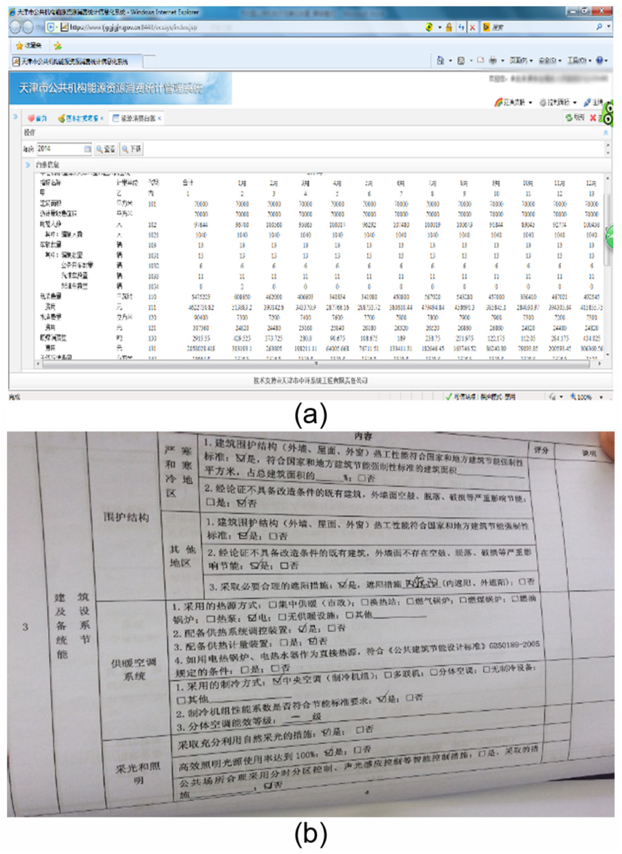
Two main sources for data access: (a) public building energy consumption and (b) questionnaire monitoring system.
Energy consumption simulation and orthogonal experiment
eQUEST is a user-friendly building energy simulation tool that provides high-quality results by combining a building creation wizard, an energy efficiency measure wizard, and a graphical results display module. 22 An eQUEST building simulation was used to perform detailed analyses and study the impact factor of office building energy consumption in Severely Cold Regions.
Orthogonal experimental design is a multi-factorial, multi-level experimental design method. It is based on orthogonality selected from comprehensive tests of certain representative points; these representative points have “evenly dispersed, neat features.” Orthogonal experimental design is the main method used for fractional factorial design. It is an efficient, rapid, and economical method for the design of experiments. Using the typical public building in the Severely Cold Regions as an example, this work will analyze the influence of various factors on office building energy consumption with the orthogonal experimental method. In section “Case study analysis of office buildings’ energy consumption influencing factor,” to provide a more intuitive and effective analysis of the data, the equivalent electrical method 23 is used to convert the energy consumption into total energy consumption.
Static data analysis
Basic information for the buildings
As shown in Table 8 in Appendix 2, the 56 buildings comprise a total construction area of 118.95 × 10⁴ m2. The total area of the government office buildings is 49.9 × 10⁴ m2, and the total area of the non-governmental office buildings is 69.05 × 10⁴ m2. The power consumption per unit of construction for the 56 buildings (without heating consumption) is 23.89–153.13 kW h/(m2 a). The average power consumption per unit of construction area (without heating) is 71.76 kW h/(m2 a), and the comprehensive energy consumption per unit of construction area is 33.86 kgce/(m2 a).
The age distribution of the sample of office buildings used in this research, as measured by the completion time shown in Figure 3, is as follows. The period before 1990 (including 1990) has four buildings, representing 7.14% of the survey. The period from 1990 to 1995 has two buildings, accounting for 3.57% of the survey, and the period from 1995 to 2000 has 13 buildings, accounting for 23.21% of the survey. For the period from 2000 to 2005, there are 11 buildings, representing 19.64% of the survey, and for the period from 2005 to 2010, there are 22 buildings, accounting for 39.29% of the survey. The period since 2010 has four buildings, accounting for 7.14% of the survey.

Age distribution of the buildings.
As shown in Figure 4, eight buildings have a construction area below 5000 m2, which accounts for 14.29% of the total area of the buildings being researched. Eighteen buildings have an area from 5000 to 10,000 m2, at 32.14% of the total. Eight buildings have an area from 10,000 to 15,000 m2, at 14.29% of the total. Four buildings have an area from 15,000 to 20,000 m2, representing 7.14% of the total, and four buildings have an area from 20,000 to 30,000 m2, accounting for 7.14% of the total. Fourteen buildings have an area of more than 30,000 m2, for 25% of the total construction area. Although the distribution of the construction area is uneven between non-governmental and government office buildings, the following analysis does not take this into account.

Area distribution of the buildings.
Electricity consumption of the buildings
The principal energy type used in the buildings under investigation is electricity. The measurements and statistics associated with the total amount of electricity consumption are relatively complete, but the data for the power consumption at the sub-meter scale are not complete. The annual energy consumption index of the different building units can be obtained from a statistical analysis of the provided power data.
After completing research on the survey data, the construction unit area of annual electricity consumption is in the range of 23.89–153.13 kW h/(m2 a). The electricity consumption for the average government office building is 31.41–122.42 kW h/(m2 a), with an average value of 76.56 kW h/(m2 a). The electricity consumption for the average non-governmental office building is 23.89–153.13 kW h/(m2 a), with an average of 68.14 kW h/(m2 a). In addition, the energy intensity frequency distribution is shown in Figure 5.

Electricity consumption distribution of the buildings: (a) non-government office buildings and (b) government office buildings.
The non-governmental office buildings’ electricity consumption is mainly concentrated in the range of 40–100 kW h/(m2 a), and that of government office buildings is concentrated in the range of 40–80 kW h/(m2 a). Because date of construction and building energy consumption are closely related, the electricity consumption of the different non-governmental and government office buildings of different ages are analyzed in terms of the distributed construction; the results are shown in Figure 6.

Electricity consumption distribution for different ages.
As shown in Figure 6, the average energy consumption for non-governmental office buildings built prior to 2000 was much higher than those built after 2000. The annual average electricity consumption per average unit construction area was 73.53 kW h/(m2 a) before 2000 and 68.14 kW h/(m2 a) after 2000, which is a decrease of 7.3%. However, the difference in the energy consumption of government office buildings from 1995 to 2005 was minimal. The annual average electricity consumption for the average unit construction area was 65.31 kW h/(m2 a) before 2000 and 74.57 kW h/(m2 a) after 2000, which is an increase of 14.2%. The main reasons for the decline in energy consumption for non-governmental office buildings after 2000 were probably the improvement in thermal insulation performance of the building envelope and the application of energy-efficient equipment. The main reason for the increase in building energy consumption for government office buildings after 2000 was likely related to the significant increase in office equipment, along with improved requirements for indoor air quality. In general, public service facilities have been greatly improved; therefore, although the government office building maintenance structure and heat preservation performance continue to improve, the total energy consumption has still increased relative to the period before 2000.
In Figure 7, it can be seen that the average electricity consumption per unit area for buildings where the total area is below 5000 m2 is the highest, but overall consumption increases and then declines as the total area grows from 5000 to 30,000 m2. Most of the buildings below 5000 m2 are government office buildings, which also tend to be older construction with poor thermal performance in the building envelope. As the building area increases, the services needed by the building will increase, and the electricity consumption will grow.
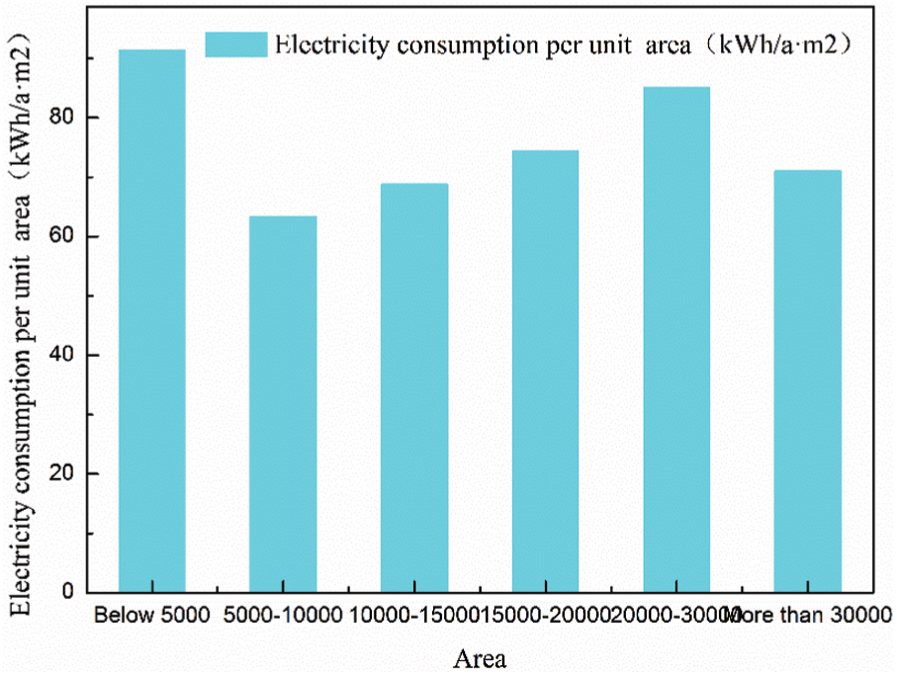
Electricity consumption distribution for different areas.
Heat supply energy consumption of the buildings
According to the research, in addition to electricity energy consumption, other major sources of energy consumption include heating, kitchens, dining rooms, and hot water, but the heating energy consumption is the largest factor. Construction in the cold region of China, which is commonly known as the northern heating region and represents approximately 70% of China’s land area, also accounts for approximately 40% of total construction for the country. Northern heating energy consumption accounts for more than 24% of the total energy consumption in China, and achieving energy savings here is the key to building energy savings in China.
The consumption of natural gas is analyzed for eight of the 56 buildings in this article that have direct-fired machine systems. The gas consumption per unit area varies widely from 0.52 to 11.16 m3/(m2 a), with an average value of 4.98 m3/(m2 a). Because the ratio of buildings analyzed to total building sample is small, results cannot reliably reflect gas heating in the severely cold area of China.
There are 31 buildings with central heating, which account for 55.36% of the total building sample and, to a certain extent, reflect the energy consumption resulting from winter heating. The annual heat consumption per unit construction area varies widely from 0.01 to 0.91 GJ/(m2 a), with an average value of 0.46 GJ/(m2 a). From the survey results, the high values for the heating energy consumption index are mainly due to the central heating construction for government office buildings, which were built in an earlier construction period, as well as the poor thermal performance of the building envelopes; in addition, many buildings do not have heat meters installed and only estimate the data (Figure 8).
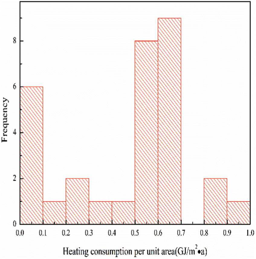
Frequency distribution of heating energy consumption per unit area.
As shown in Figure 9, the heating energy consumption for central heating shows a downward trend based on how recently the building was completed, which is mainly due to upgrades to enclosure structures and central heating efficiency. However, although the overall trend is downward, there are big fluctuations, with those buildings built from 1995 to 2005 having high-energy consumption per unit construction area because they were built before the introduction of the “design standard for energy efficiency of public buildings 2005.” 24 With the development of the economy, and because people have increasingly demanded a comfortable office environment, energy consumption for centrally heated office buildings experienced a growth trend in the years 1995–2005. With the “design standard for energy efficiency of public buildings 2005,” 24 the introduction of coal gas and the implementation of a large number of small boilers, heating energy consumption for buildings built after 2005 dropped significantly compared with those built before 2005.
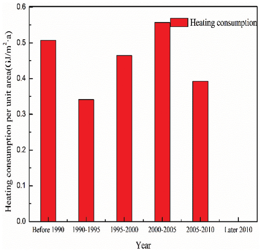
Heating consumption distribution for different building ages.
As shown in Figure 10, with the growth of the construction area, the heating energy consumption for central heating shows a downward trend, which is also mainly due to upgrades to the enclosure structure and improvements in the efficiency of central heating. Although the overall trend is downward, there is a fluctuation for buildings whose area is in the range of 10,000–15,000 m2. This is because there is only one building in that area range that uses central heating; as such, this is an outlier.

Heating consumption distribution in different areas.
Comprehensive energy consumption of the buildings
From the survey data, the overall comprehensive energy consumption during construction is in the range of 7.94–58.41 kgce/(m2 a), the comprehensive energy consumption for government office buildings is between 7.94 and 57.23 kgce/(m2 a), and the average value is 39.10 kgce/(m2 a); comprehensive energy consumption for non-governmental office buildings is 16.14–58.41 kgce/(m2 a), with an average of 29.16 kgce/(m2 a). The intensity frequency distribution for comprehensive energy consumption is shown in Figure 11. The comprehensive energy consumption for non-governmental office buildings is mainly concentrated in the range of 10–40 kgce/(m2 a), and that of government office buildings is concentrated in the range of 30–60 kgce/(m2 a).

Comprehensive energy consumption distribution of the buildings: (a) non-government office buildings and (b) government office buildings.
In Figure 12, it can be clearly seen that the comprehensive energy consumption per unit area for non-governmental office buildings and government office buildings has decreased over time. For non-governmental office buildings built after 2010, the comprehensive energy consumption per unit area compared to the same for the period 1990–1995 fell by 58.34%, whereas the energy consumption per unit area for government office buildings built after 2010 was down by 75.37% compared to 1990. The energy saving effect is obvious. The relationship between improved electricity consumption per unit area and building age is less obvious. This is mainly because although the improved thermal performance of the building envelope and energy saving appliances improved the overall energy efficiency, people’s requirements in terms of indoor environmental quality and comfort also increased. Consequently, the rapid increase in the types and quantities of electric equipment used has resulted in no significant decline in the total energy consumption per unit building area. It can be seen from Figure 13 that the comprehensive energy consumption also shows a downward trend with an increased building area. Although electricity consumption grows as the building area increases, energy consumption for heating decreases with the increased area, and that reduction is larger than the increase in energy consumption due to the increased use of electricity.

Comprehensive energy consumption consumption distribution for different ages.

Comprehensive energy distribution for different areas.
Energy consumption level of the buildings
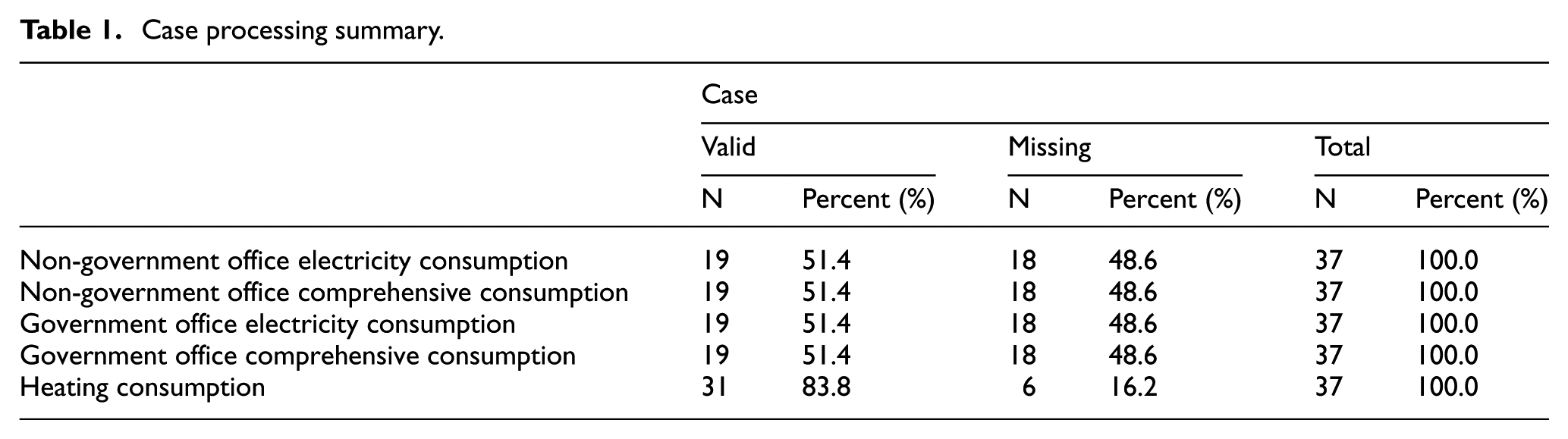
A box-whisker plot was used to reflect the level of energy consumption for the research buildings. Before using statistical methods to calculate the datum line or level, data selection and processing should be done first to remove the abnormal values. The methods that are used to judge abnormal values assume a normal distribution based on the mean and standard deviation of the data. The commonly used methods for a normal distribution are Grubbs outliers and a Z score. Most of the data, however, do not strictly obey the normal distribution, so the effectiveness of these methods is limited. Instead, a box line is applied; a box line (Box plot), also known as the box (Box–whisker plot), is a kind of statistical plot that shows data dispersion. To describe the distribution of the data, the box line graph uses five statistics from the data: the minimum value, the first four points (Q1), the median (Q2), the first three or four points (Q3), and the maximum value. The degree of dispersion of the data and outliers in the data can be broadly seen to determine the bias of the data. A case processing summary and a schematic diagram of the box line plot are shown in Table 1 and Figure 14.
Case processing summary.

Box–whisker plot of the buildings.
The center position of the box plot data shows the median; the upper and lower case on the data of the four digits (Q3) and four digits (Q1) between Q3 and Q1 shows a distance called the four points distance (interquartile range (IQR)); the two ends should show the maximum and minimum values of the data. The standard for judging whether a value in the box line is abnormal is whether it is less than Q1–1.5IQR or more than Q3+1.5IQR. Test results can be seen in the figure as less-abnormal data in the box line graph, except for the comprehensive energy consumption value of a non-governmental office building and excluding a data label for 14.
At the same time, it can be seen from Figure 14 that non-governmental office buildings’ electricity consumption, comprehensive energy consumption, and government office building electricity consumption, which are the three indicators in the abdomen, are more uniform. Additionally, the two indexes for comprehensive energy consumption and heating energy consumption for government office buildings are small, between the median and 75% (fourth quartile). This result suggests that for the investigation of the building, these two indicators constitute more than 25%–50% in this range, whereas the other three indicators are more evenly distributed in the range of 0%–100%. At the same time, from Figure 14 and Table 2, it can be seen that the mean of these two indicators for electricity consumption per unit area and heating energy consumption for government office buildings exhibits a large difference between the mean and the average. The other three indicators have a smaller gap between the average and the median value.
Case processing result.

The existence of multiple modes. Display minimum.
Uncertainty factor analysis
1. Level of management is different
The building energy consumption is different for different system management levels. Research on buildings with a relatively high level of preservation of the building’s original information is robust, as building personnel typically have a good mastery of basic building information, such as the operation of the building, equipment, and number of personnel. However, the actual operations and management systems of some construction are relatively weak, and the relevant documented information is poorly arranged, resulting in data loss and reduced data reliability.
2. Data collection is different
Basic data are required to carry out any work, but system monitoring, measurement, statistics, and other aspects of energy consumption are relatively weak in China. Whether for statistical methods or for time interval statistics, it is very difficult to find a unified standard. This results in a lack of unified data for energy consumption, while enhancing the contradictory nature of energy consumption statistics.
3. Limited number of samples, building information, and energy consumption data
Due to the limited number of samples and the lack of basic information and energy consumption data, some data cannot fully reflect office building energy consumption for the cold areas of China.
Case study analysis of office buildings’ energy consumption influencing factor
To further analyze the energy consumption influence factor for office buildings, the paper choose one typical building to research. The simulation software eQUEST was used in the study.
Target buildings and building description
In Model 1 architecture, three floors underground are used for parking garages, levels 1–2 are mainly for commercial use, and levels 3–12 are mainly for office use. The basic information for the buildings can be seen in Table 3 and the 3D models in Figure 15.
Building basic information.


Building models of 3D.
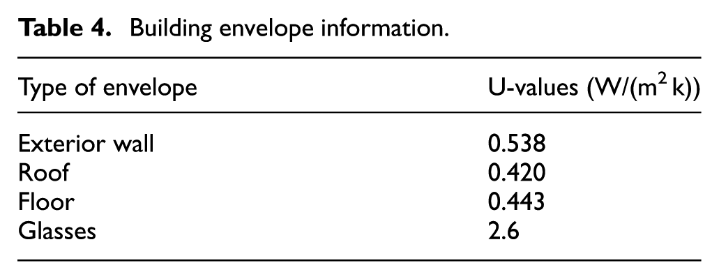
The parameters of the building envelope are shown in Table 4.
Building envelope information.
In addition to indoor light, equipment, and other initial conditions are parameters that affect the building’s energy consumption. Indoor light, equipment, and other initial conditions are shown in Table 5.
Indoor light, equipment and other initial conditions.

The parameters of building Heating,Ventilating and Air Conditioning (HVAC) system are shown in Table 6.
Air-conditioning system information.

CAV: constant air volume; COP: coefficient of performance.
Model calibration
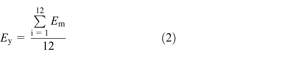
Calibrating the model is an important part of building an energy consumption simulation. According to the literature,25–27 a common method to verify the model is to compare it with the actual energy consumption data of a building. The calculation formula and the acceptable error range of month error Em, year error Ey as well as the variance coefficient of variation δm are given in the previous study.25–27 The smaller these three numbers are, the more reliable the model is. The calculation methods of the three coefficients are as follows

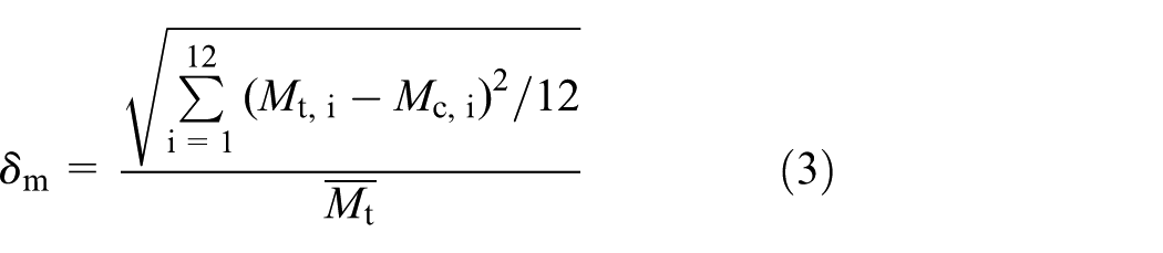
where Mt,i represents building I’s months of actual energy consumption, Mc,i represents building I’s months of simulation of energy consumption, and
The verification results of the energy consumption models are shown in Figure 16. The short line in the graph is the limit error of the line 15% between simulated and actual energy consumption error provisions in the document (Figure 16). 26

Comparison between simulated and actual energy consumption.
According to formulas (1)–(3), the calculation results are shown in Table 7: the maximum deviation of the Em month of the building as it appeared in July is 8.26%, the year deviation coefficient is Ey = 4.40%, and the variance coefficient variation is δm = 5.07% months. The deviation coefficient table is within the acceptable error range in the literature25–27 compared with the model. Although the model does not meet the delta δm within the 26 literature limits, the other limits can satisfy other values in the literature. This shows that the typical building energy models can be used to represent the actual situation, and that the actual deviation is smaller, with good reliability.
Comparison of two building simulation errors and the range of acceptable error.
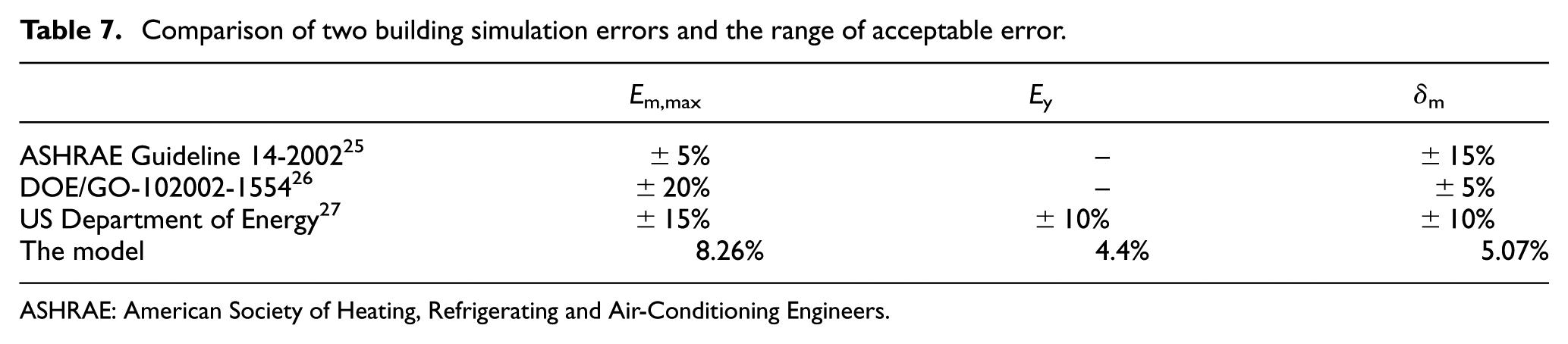
ASHRAE: American Society of Heating, Refrigerating and Air-Conditioning Engineers.
Orthogonal experiment
While there are many influence factors for the energy consumption of office buildings, they can generally be divided into two categories: external and internal causes. External causes refer to various kinds of interference with the indoor thermal environment, which includes two parts of the inner disturbance and outside disturbance. Inner disturbance refers to the changes of the human body and equipment heat, moisture dissipation, and lighting heat dissipation of an inside room. Outside disturbance refers to weather factors, such as changes in outdoor air temperature, humidity, solar radiation intensity, and wind speed and direction. Internal causes mainly refer to the condition of the building itself, including building orientation, and to palisade structure parameters such as structure and shape coefficients.
Office building energy consumption composition mainly includes the energy consumption of air conditioning, lighting, and equipment; the influence factors corresponding to that are air conditioning, lighting, and equipment energy consumption.
The paper mainly studies the following factors that affect the energy consumption of office buildings: window-wall ratio, wall type, window type, occupancy density, lighting equipment load, roof type, shading coefficient and indoor set temperature, air index and air-conditioning system forms, and chiller coefficient of performance (COP). To confirm the influence degree of various factors on the results, two representative indexes and two typical buildings were selected. The design and results of orthogonal test table can be seen in Table 9 in Appendix 2.
According to the range of relative size of influence, the order of factor importance is air-conditioning system > lighting density > indoor design temperature > exterior window type > outside shading > fresh air volume > personnel density > roof type > COP of refrigerating unit > window-wall ratio > exterior wall type. The analysis results show that the influence of the air-conditioning system is the largest, followed by lighting density and the building envelope. Thus, the paper analyzes these factors.
Enclosure structure
Exterior wall
The wall is a very important part of the building envelope. The heat enters the room through the wall structure through two major paths: the convection heat transfer between the outdoor air and the enclosure structure and the solar radiation heat transfer through the wall.
According to the needs of the research, five different heat transfer coefficients for the external walls of the model were selected for simulation and analysis. The influence on the total energy consumption is shown below.
With an increase in the exterior wall heat transfer coefficient, the total annual energy consumption, electricity consumption, and gas consumption for heating all increased basically linearly. The effect of different exterior wall heat transfer coefficients is obvious on the total energy consumption, electricity, and gas consumption. As shown in Figure 17, the increase in gas consumption is the most obvious. The total energy consumption of the two models increased most obviously during winter, which also means that the exterior wall heat transfer coefficient change has a huge effect on the heating energy consumption.

Variables of energy consumption, electricity consumption, and gas consumption for heating in different exterior wall U-values.
Some things can be calculated using the data in Figure 17. In the model, when the exterior wall heat transfer coefficient rises from 0.5 to 2.5 W/(m2 k), the total energy consumption grows from 3933.01 × 103 to 4251.73 × 103 kW h, increasing by 8.1%. Thus, when the heat transfer coefficient of the exterior wall of the first modeled building increases 1 W/(m2/K), the total energy consumption per unit area of the building rises 4.44 kW h(m2 a). Electricity consumption grows from 3748.6 × 103 to 3974 × 103 kW h, increasing by 6.01%. Gas consumption rises from 629.17 × 10⁶ to 947.56 × 10⁶ btu, growing by 50.6%; this growth is very obvious. The change in the exterior wall heat transfer coefficient has the greatest impact on gas consumption for heating.
Exterior window
For building energy savings, doors and windows are the key. In summer, blocking the heat of the outdoor to indoor conduction can maintain an indoor refrigeration effect, whereas in winter, this can reduce the loss of indoor heat. In this process, doors and windows play a key role.
According to the needs of the research, five groups of different heat transfer coefficients for the external windows were selected for simulation and analysis. As seen from Figure 18, the influence of exterior window heat transfer coefficient changes for total energy consumption, building energy consumption, and power consumption of heating gas is obvious. The pictures show that with an increase in the exterior window, heat transfer coefficient, the total energy consumption, electricity consumption, and gas heating energy consumption of the two models decrease during May–September but increase in November–January. This is mainly because May–September belongs to the cooling season for two models. Furthermore, because thermal inertia exists in the building materials, the outdoor temperature is lower than the indoor temperature at night, so a smaller coefficient of thermal conductivity is not conducive to heat release from indoors to outdoors. This requires interior air conditioning to release the increased heat during the day and causes a greater heat increase than the reduced daytime heat gain with an improved exterior glass thermal insulation performance; thus, the energy consumption increases.

Variables of energy consumption, electricity consumption, and gas consumption in different glass U-values.
With an increase in the exterior window heat transfer coefficient, the total energy consumption and gas consumption increased basically linearly, and the electricity consumption showed a trend of decline. The results can be calculated using the data in Figure 18. In the model, when the exterior window glass heat transfer coefficient increased from 1.8 to 5.5 W/(m2 k), the total energy consumption grew from 3903.391 × 103 to 3967.999 × 103 kW h, an increase of 1.66%, representing limited growth. The effect of the exterior window heat transfer coefficient on total annual energy consumption is limited, and economies should be fully considered while saving energy. Electricity consumption fell from 3736.6 × 103 to 3705.9 × 103 kW h, a decrease of 0.82%, whereas gas consumption increased from 569.06 × 10⁶ to 894.23 × 10⁶ btu, with a very obvious growth of 57.14%.
Lighting and equipment
Lighting power density
According to the results of the orthogonal test for the model in section “Orthogonal experiment,” the lighting power density factor is the second most influential factor, following the air-conditioning system factors.
The paper uses five different lighting power densities for the simulation analysis. In the model, total energy consumption and power consumption present basic linear growth with respect to increments of lighting power density, and the gas consumption presents a straight decline. This is mainly due to the heating season: with an increase in the power density of the lighting, the heat capacity of the equipment increases to reduce gas consumption and achieve the required design temperature. Conversely, during the cooling season, there is a need for greater power consumption, which increases the electricity consumption, to achieve colder summer indoor design temperatures. During the transition season, lighting power density also increases the electricity consumption of the building itself.
Further results can be calculated using the data in Figure 19. For the model, when the lighting power density rises from 6 to 14 W/m2, the total energy consumption increases from 3697.402 × 103 to 4308.087 × 103 kW h, an increase of 16.52%. Electricity consumption, which went from 3495.6 × 103 to 4148.6 × 103 kW h, grew by 18.68%. Gas consumption dropped from 688.51 × 10⁶ to 544.14 × 10⁶ btu, falling by 20.97%.
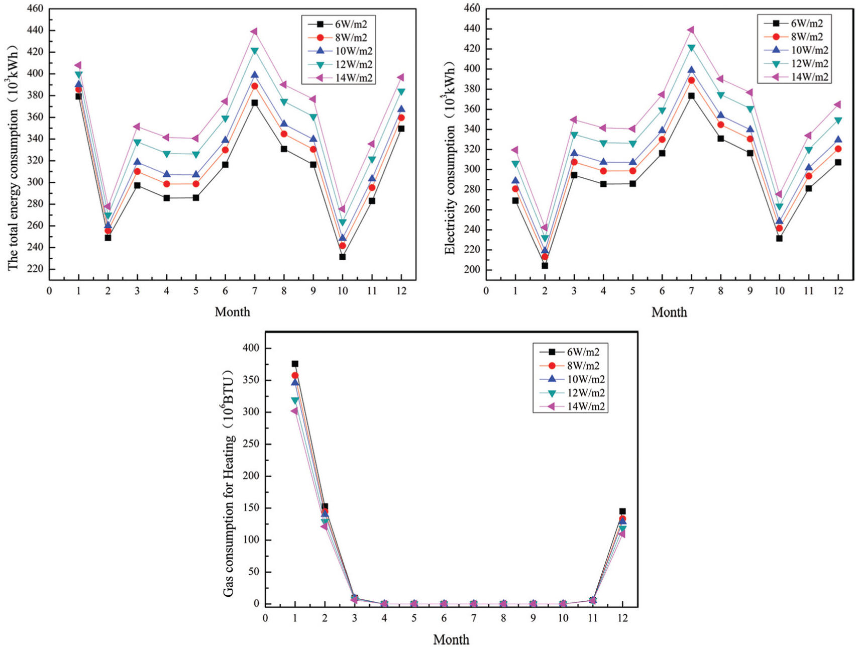
Variables of energy consumption, electricity consumption, and gas consumption in different lighting power densities.
Equipment power density
The effect of office equipment power density on the energy consumption of buildings is similar to that of lighting density. Along with an increase in device power density, the total energy consumption and electricity consumption present basic linear growth, and the gas consumption presents a straight decline, as shown in the model. This is mainly due to the heating season, for which an increase in the power density of the office equipment causes the heat capacity of the equipment to increase, thereby reducing gas consumption and achieving the required design temperature. However, for the cooling season, to obtain a cold indoor design temperature in summer, more power must be consumed, thereby increasing the electricity consumption. In the transition season, the lighting power density increases also increases the electricity consumption of the building itself.
The data in Figure 20 are used for calculation. In the model, when the office equipment power density rises from 11 to 19 W/m2, the total energy consumption increases from 3741.164 × 103 to 4161.837 × 103 kW h, increasing by 11.24%. Electricity consumption increases from 3532.7 × 103 to 4002.2 × 103 kW h, growing by 13.29%. Gas consumption decreases from 711.24 × 10⁶ to 544.65 × 10⁶ btu, falling by 23.42%.
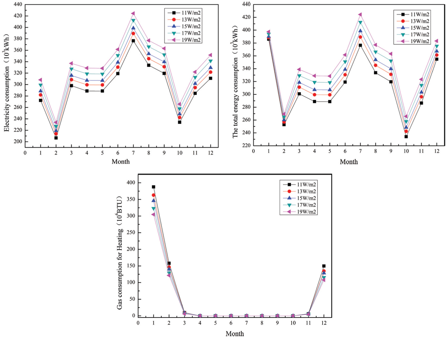
Variables of energy consumption, electricity consumption, and gas consumption in different equipment power densities.
Air-conditioning system
Ground source heat pumps (GSHP) involve the use of shallow land energy through the input of a small amount of high-grade energy (such as energy) to achieve energy from a low-grade to high-grade heat transfer. The GSHP is one of the most current and mature technologies for use of renewable energy in air conditioning and as a heat source. Therefore, by setting a GSHP as a building’s cold and heat source (with a variable air volume (VAV) air-conditioning system), and comparing these results with the energy use of a non-GSHP constant air volume (CAV) air-conditioning system, VAV and variable refrigerant volume (VRV) air-conditioning system, the simulation results below can be generated. For the non-GSHP data, the common centrifugal chiller is used as the cold source and the gas-fired boiler as the heat source for CAV and VAV.
Figure 21 clearly shows that the building’s total energy consumption and electricity consumption are smaller than those of CAV and VAV but slightly greater than that of VRV. The CAV all-air system is the largest energy consumer, which is mainly caused by the too-large fan energy consumption. The model’s total energy consumption when using CAV is 3933.01 × 103 kW h, while VAV is 2750.78 × 103 kW h, GSHP is 2536.40 × 103 kW h, and that of VRV is only 2389.7 × 103 kW h. Relative to the CAV system, the energy saving rate is 39.24%. Using a GSHP as the cold and heat source, the total energy consumption is lower than that of the centrifugal chiller and gas boiler as cold and heat sources for CAV and VAV but slightly higher than that of VRV. Different air-conditioning systems’ energy consumption simulation found that the air-conditioning system had a huge impact on the building energy consumption, and overall, the energy efficiency of the GSHP system is still quite obvious.
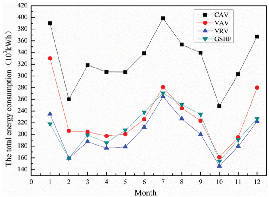
Variables of energy consumption and electricity consumption in different air-conditioning systems.
Uncertainty factor analysis
Although the overall results of the simulation verify the accuracy of the model and the typical building basically meets all of the indicators, there is still some error. The causes for this deviation include the following:
The software master is not very good, with mobile errors;
The running times of various equipment and personnel in the documentation are inconsistent with their actual operation;
Because the wide variety of equipment often cannot match a specific system’s parameters, longer service life and other issues can occur, leading to decreased equipment performance; and
When using meteorological parameters to simulate typical parameters, the meteorological parameters may exhibit certain discrepancies.
Conclusion and suggestions
Conclusion
Using typical public buildings in severe cold and cold regions as examples for the work analysis and study of the energy consumption situation, the influence factors of office building energy consumption were found using an orthogonal experiment method. In this research, the basic information and energy consumption data for 56 typical office buildings are investigated, including 19 non-government office buildings and 37 government office buildings. According to the investigation data, the energy consumption situation and some factors that influence energy consumption were analyzed. Through an orthogonal experiment, the author selected the exterior wall of the building’s heat transfer coefficient, as well as the heat transfer coefficients of the external windows and lighting equipment, the power density, and the power density of the air-conditioning system as five of greatest impact factors for building energy consumption for further analysis and study. The simulation software eQUEST was used in the study. Energy saving measures were put forward according to the results of the analysis and study.
According to the survey data, the construction unit construction area of annual electricity consumption ranges from 23.89 to 153.13 kW h/(m2 a); the government office building electricity consumption is in the 31.41–122.42 kW h/(m2 a) range, with an average value of 76.56 kW h/(m2 a); non-government office building electricity consumption is in the 23.89–153.13 kW h/(m2 a) range, with an average of 68.14 kW h/(m2 a). In addition, the non-government office buildings’ electricity consumption is mainly concentrated in the 40–100 kW h/(m2 a) range, whereas that of government office buildings is concentrated between 40 and 80 kW h/(m2 a).
In the research of 56 buildings, for 8 buildings with direct-fired machine systems, the consumption of natural gas was analyzed, and the gas consumption per unit area was in the 0.52–11.16 m3/(m2 a) range with huge differences; the average value was 4.98 m3/(m2 a). Overall, 31 buildings with central heating accounted for 55.36% of the total number of samples and, to a certain extent, reflected the energy consumption of winter heating. The unit construction area of annual heat consumption is in 0.01–0.91 GJ/(m2 a) with huge differences, and the average value is 0.46 GJ/(m2 a).
From the survey data, the comprehensive construction energy consumption ranges from 7.94 to 58.41 kgce/(m2 a); the government office buildings’ comprehensive energy consumption is 7.94–57.23 kgce/(m2 a) with an average value of 39.10 kgce/(m2 a); and non-government office buildings’ comprehensive energy consumption is 16.14–58.41 kgce/(m2 a) with an average of 29.16 kgce/(m2 a). In addition, the non-government office buildings’ comprehensive energy consumption is mainly concentrated in the 20–40 kgce/(m2 a) range, whereas that of government office buildings is concentrated in the 30–60 kgce/(m2 a) range.
The two indexes of government office buildings’ comprehensive energy consumption and heating energy consumption are smaller between the median and 75% (fourth percentile). This result suggests that for the investigation of the building, the influence from these two indicators is more in the 25%–50% range, whereas the other three indicators are more evenly distributed in a range from 0% to 100%. At the same time, when these results are combined with those of Figure 13 and Table 3, it becomes clear that the mean of these two indicators of government office building electricity consumption per unit area and heating energy consumption have a large difference between the mean and average, whereas the other three indicators show a smaller gap between the average and median values.
The paper analyses and studies the factors that affect the energy consumption of office buildings using an orthogonal experiment method. A deviation coefficient table with acceptable error ranges from the literature25–27 was compared with the model. Although the model does not meet the delta δm in the 26 literature limits, the other limits satisfy all three values in the literature. This shows that the typical building energy models can be used to show the actual situation, and that the actual deviation is smaller, with good reliability.
According to the range of results for relative size of influence, the order for the building’s influential factors is air-conditioning system > lighting density > indoor design temperature > exterior window type > outside shading > fresh air volume > personnel density > roof type > COP of refrigerating unit > window–wall ratio > exterior wall type. Through analysis, it was found that the air-conditioning system is the most influential impact factor, followed by the lighting equipment and the building envelope.
With the increase in the exterior wall heat transfer coefficient, the total annual energy consumption and electricity and gas consumption increased nearly linearly; with an increase in the exterior window heat transfer coefficient, total annual energy consumption and gas consumption increased nearly linearly, but the electricity consumption was decreased; and with an increase in the lighting power and office equipment density, the total annual energy consumption and electricity consumption had a linear growth trend, but the heating gas consumption decreased. The use of GSHP as a cold and heat source air-conditioning system consumes less energy than the CAV and VAV and slightly more than the VRV.
Suggestions
An analysis of the results indicates that the main factors affecting the energy consumption of buildings are the building envelope, lighting equipment, office equipment, and air-conditioning system. Therefore, the article puts forward the following suggestions:
To minimize the heat transfer coefficient of the exterior walls and windows, an appropriate reduction of the heat transfer between the indoor environment and the outdoor air is indicated.
Replace lighting with energy saving lamps, reducing the lamp power density. A large number of old T8 lamps are currently being used in some office buildings in China.
To improve the energy management system, office users should form the habit of turning off the lights when they leave and using fewer lights to satisfy illumination needs when possible, reducing the power consumption of lighting lamps.
Turn off the computer, printer, and other office equipment in a timely manner, in order to reduce their power consumption.
Where there is a choice in the appropriate form of air-conditioning system, attempt to the limit possible to avoid using high-energy consuming air-conditioning systems.
To the extent possible, use renewable energy sources to reduce the pollutant emissions and energy consumption of buildings.
Footnotes
Appendix 1
Appendix 2
Orthogonal experiment design and result of the model.

| 1 |
2 |
3 |
4 |
5 |
6 |
7 |
8 |
9 |
10 |
11 |
12 |
|
|---|---|---|---|---|---|---|---|---|---|---|---|---|
| Window–wall ratio | Exterior wall (W/m2 k) | Exterior window (W/m2 k) | Occupancy density (m2/person) | Lighting power density (W/m2) | Roof type (W/m2 k) | External sunshade | Indoor design temperature (°C) | Fresh air volume (m3/(h person)) | Air-conditioning system | COP of refrigerating unit | Result (104 kW h) | |
| Experiment1 | 0.4 | 0.538 | 2.6 | 8 | 9 | 0.42 | No | 26 | 30 | Constant air volume | 5.2 | 393.29 |
| Experiment2 | 0.4 | 0.538 | 2.6 | 8 | 9 | 0.326 | Yes | 24 | 20 | Variable air volume | 4.2 | 279.07 |
| Experiment3 | 0.4 | 0.538 | 1.8 | 4 | 7 | 0.42 | No | 26 | 20 | Variable air volume | 4.2 | 261.34 |
| Experiment4 | 0.4 | 0.404 | 2.6 | 4 | 7 | 0.42 | Yes | 24 | 30 | Constant air volume | 4.2 | 388.16 |
| Experiment5 | 0.4 | 0.404 | 1.8 | 8 | 7 | 0.326 | No | 24 | 30 | Variable air volume | 5.2 | 272.09 |
| Experiment6 | 0.4 | 0.404 | 1.8 | 4 | 9 | 0.326 | Yes | 26 | 20 | Constant air volume | 5.2 | 374.56 |
| Experiment7 | 0.4 | 0.538 | 1.8 | 4 | 9 | 0.42 | Yes | 24 | 30 | Variable air volume | 5.2 | 286.29 |
| Experiment8 | 0.3 | 0.538 | 1.8 | 8 | 7 | 0.326 | Yes | 26 | 30 | Constant air volume | 4.2 | 358.95 |
| Experiment9 | 0.3 | 0.538 | 2.6 | 4 | 7 | 0.326 | No | 24 | 20 | Constant air volume | 5.2 | 388.33 |
| Experiment10 | 0.3 | 0.404 | 1.8 | 8 | 9 | 0.42 | No | 24 | 20 | Constant air volume | 4.2 | 387.76 |
| Experiment11 | 0.3 | 0.404 | 2.6 | 4 | 9 | 0.326 | No | 26 | 30 | Variable air volume | 4.2 | 285.98 |
| Experiment12 | 0.3 | 0.404 | 2.6 | 8 | 7 | 0.42 | Yes | 26 | 20 | Variable air volume | 5.2 | 257.74 |
| Mean1 | 328.09 | 327.88 | 332.09 | 324.82 | 334.49 | 329.10 | 331.47 | 321.98 | 330.79 | 381.84 | 328.72 | |
| Mean2 | 327.51 | 327.72 | 323.50 | 330.78 | 321.10 | 326.50 | 324.13 | 333.62 | 324.80 | 273.75 | 326.876 | |
| Range | 0.579 | 0.163 | 8.595 | 5.960 | 13.39 | 2.602 | 7.338 | 11.643 | 5.995 | 108.089 | 1.840 |
COP: coefficient of performance.
Acknowledgements
The authors also would like to acknowledge Ministry of Environment Protection of the People’s Republic of China and School of Environmental Science and Engineering of Tianjin University in supporting our building energy audit and providing valuable comments for this research.
Handling Editor: Oronzio Manca
Declaration of conflicting interests
The author(s) declared no potential conflicts of interest with respect to the research, authorship and/or publication of this article.
Funding
The author(s) disclosed receipt of the following financial support for the research, authorship and/or publication of this article: This research was funded by the State Nuclear Electric Power Planning Design & Research Institute Support Key Project under grant number 100-KY2017-FYZ-N01 and by the Beijing Municipal Science and Technology Project under grant number Z171100000317004.