
Abstract
Mesh partitioning is significant to the efficiency of parallel computational fluid dynamics simulations. The most time-consuming parts of parallel computational fluid dynamics simulations are iteratively solving linear systems derived from partial differential equation discretizations. This article aims at mesh partitioning for better iterative convergence feature of this procedure. For typical computational fluid dynamics simulations in which partial differential equations are discretized and solved after the mesh is partitioned, numerical information of the linear systems is not available yet during mesh partitioning. We propose to construct approximations for matrix elements and theoretically find out that for finite-volume-based problems, the face area can approximate the corresponding matrix element well. A mesh partitioning scheme using the matrix value approximations for better iterative convergence behavior is implemented and numerically testified. The results show that our method can capture the most important factor influencing the matrix values and achieve partitions with good performance throughout the simulations with non-uniform meshes. The novel partitioning strategy is general and easy to implement in various partitioning packages.
Keywords
Introduction
It is widely known that large-scale computational fluid dynamics (CFD) simulations usually require a large amount of computational effort. Therefore, parallel computing is introduced to help solve these problems within acceptable time. For a parallel CFD problem, the core procedure is solving the partial differential equations (PDEs) in parallel. In many CFD platforms such as Fluent Inc. 1 and OpenFOAM, 2 in the pre-processing phase, mesh is first generated from the geometry and then partitioned into several sub-domains. The governing equations are discretized on the partitioned mesh and the problem is eventually transformed into solving a sequence of linear systems in parallel. In general, up to 80% of the CPU time for a flow solver is spent on solving the linear systems 3 which becomes the major bottleneck of the overall efficiency.
Preconditioned iterative solvers are popular methods for solving linear systems. How the mesh is partitioned is significant to the performance of parallel preconditioned iterative solvers.4–8 The number of iterations depends on the choice of partition because the numerical characteristic of the preconditioned matrix varies under different partitions.9–12 Duff and Koster,9,10 Duff et al., 11 and Sosonkina et al. 12 are the most representative works on partitioning aiming at efficient parallel preconditioners for a known linear system. The partition tries to involve the most relevant information of the matrix in the diagonal blocks to increase the diagonal dominance of the permuted linear system. Thus, the magnitudes of matrix entries are taken into account and large off-diagonal entries moved into diagonal blocks as much as possible by so-called matrix reordering. 9 One simple and effective way to implement this is to use an adjacency graph to represent the pattern of the matrix and consider weights assigned to the edges of the graph, where the weights are determined by the coefficients of the matrix. 13
However, considering the matrix information during the static mesh partitioning is not feasible since the PDEs have not been discretized into linear systems yet. As far as we know, if the matrix nonzero values are to be taken into account, some kind of dynamic load balancing method should be adopted during the simulation. Given that the matrix nonzero values might change a lot throughout the simulation of complex fluid dynamics, dynamically repartitioning the mesh along with the timesteps can be quite expensive. Working on dynamically repartitioning strategies is beyond the scope of this article.
We consider the problem of static mesh partitioning at the beginning of the parallel CFD simulations. Inspired by the work of matrix partitioning aiming at efficient parallel preconditioners, we try to roughly build approximations for matrix nonzero entries throughout the simulation and adopt them in the mesh partitioning. The load balance and communication overhead are also taken into account. The partition is performed only once and efficient parallel preconditioners can be expected throughout the whole simulation. The main contributions of this article include the following:
This article brings forward the idea of constructing approximations for matrix values on the mesh topology. Thus, mesh partitioning considering the numerical characteristic of the coefficient matrix of linear system can be conducted at the beginning of the simulation.
For CFD problems using finite volume method (FVM), we analyze the discretization of a PDE into a linear system and find out that the areas of the interfaces are appropriate approximations for the matrix off-diagonal coefficients. A generalized partitioning model combining load balance, communication volume, and convergence feature using the matrix value approximations is built.
The face-area-based partitioning model is implemented based on Metis. An adjacency graph is constructed from the mesh topology and the face areas are assigned to the graph edges as weights. The edge-weighted graph can be partitioned by the existing graph partitioning routines in Metis. This new partitioning scheme is named as FMetis (Face-area based Metis).
Four CFD problems are established to numerically testify FMetis. The results show that it significantly outperforms the original Metis partitioning method with no weights on the edges. Comparing with the partitioning method which directly uses the matrix coefficients as the edge weights, FMetis shows a similar performance and sometimes even better for non-uniform meshes. Compared with dynamically repartitioning the mesh every timestep, FMetis exhibits a competitive performance throughout the simulation in terms of the iterative convergence rate.
FVM-based mesh partitioning
There are two important issues when we attempt to use matrix value approximations in mesh partitioning for better iterative convergence feature:
How should we indicate the matrix values on the mesh level before the PDE discretization? Specifically, we should work out easy and appropriate approximations for the values of off-diagonal matrix entries derived from the discretization on the mesh.
What are the proper partitioning model using matrix value approximations and how can the partitioning be performed in practice?
Approximations of matrix coefficients
To approximate matrix off-diagonal entries on the mesh, we should figure out how they are derived from the discretization of governing equations. We concentrate on cell-centered FVM in which the control volumes are formed by the mesh cells with the cell centers “storing” the average variable values. The face fluxes are approximated using the variable values in the two adjacent cells surrounding the face in central differencing (CD) scheme.
Considering the standard form of the transport equation for a scalar property

where
A finite volume discretization of the equation is formulated by integrating over the control volume
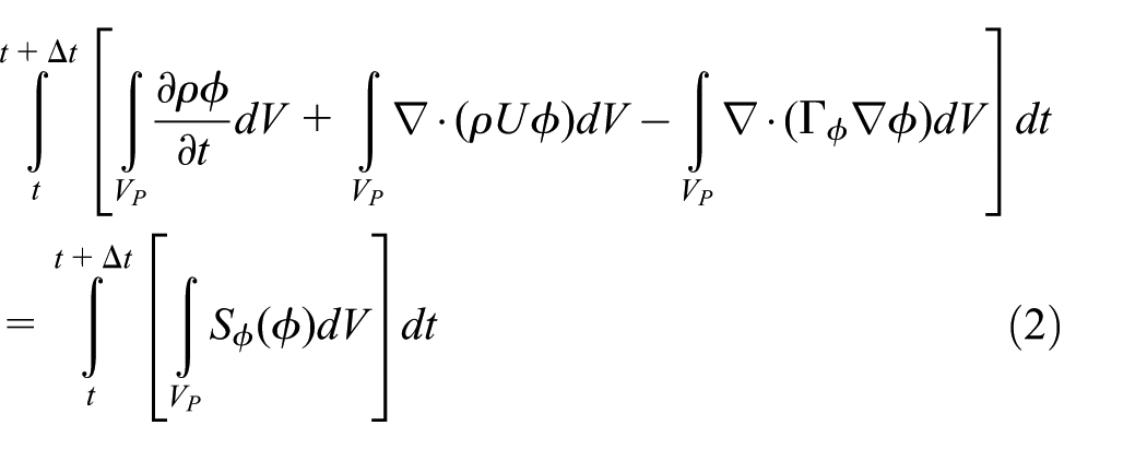
We work on the discretization procedure in one timestep and others can be analyzed in the same way. Most of the spatial derivate terms of equation (2) are converted to integrals over the surface S bounding the volume using the generalized form of Gauss’s theorem

where f is a face belonging to S. The value

P and N are the two cells that own f and
Equation (1) will be transformed in terms of

An illustration of an internal face f and its owner cells P and N in finite volume discretization.
Now, how
Time derivative
Discretization of the time derivative is performed by integrating it over the cell P
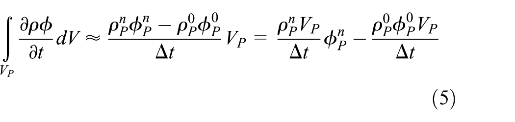
where
Convection term
Discretization of the convection term is performed by integrating it over the cell P and transforming the volume integral into a surface integral using the Gauss’s theorem

For face f between cell P and cell N, according to equation (4), we have

The coefficient term of
Diffusion term
Discretization of the diffusion term can be done in a similar way to the convection term

Considering the most frequently used orthogonal mesh, that is, vector d and

where
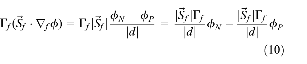
Similar to the convection term, discretization of the diffusion term over a cell P also contributes to the diagonal entry
Source term
The source term can be a general function of

where
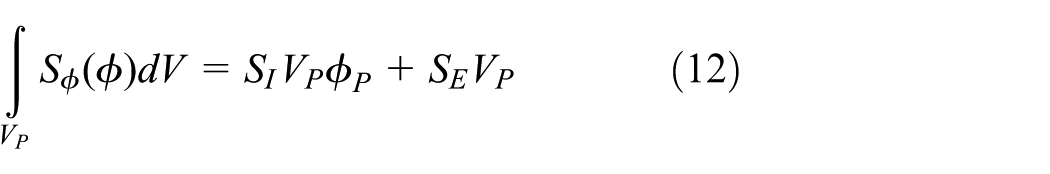
Obviously, equation (12) contributes to the diagonal entry
Summarization
According to equations (5), (7), (10), and (12),
Partitioning model and its implementation
Normally, graph partitioning models are used to conduct mesh partitioning. Cells and faces of the mesh are formulated by vertices and edges of the graph, respectively. We use the face areas to approximate the corresponding matrix off-diagonals and assign them as edge weights in the graph partitioning model. Combining load balancing and communication overhead, the novel mesh partitioning problem aiming at better iterative convergence rate can be formulated as a variant of the standard graph partitioning model as follows. Given a graph
where
Our partitioning model is a straight-forward variant of the traditional graph partitioning model Karypis and Kumar.19,20 There are plenty of packages that can be adopted to implement our partitioning model. Considering that graph partitioning has been studied quite well, we solve our partitioning problem with a general and well-known multilevel k-way graph partitioning tool: Metis. 21 For the reason that the most important characteristic of our method is using Metis with face areas as edge weights, we name the method as FMetis (Face-area-based Metis). A graph is first constructed from the mesh topology. The face areas are then assigned to the corresponding graph edges as weights. The edge-weighted graph can be partitioned using Metis.
To partition a graph with Metis, the graph should be stored in the compressed storage format (CSR). For a graph

where adjncy stores the adjacency vertices list for each vertex and the array xadj is used to index adjncy. vwgt and adjwgt record the weights for n vertices and m edges, respectively. Notice that each edge and its weight are recorded twice in adjncy and adjwgt, respectively.
The implementation of mesh partitioning with FMetis is presented in Algorithm 1. The corresponding adjacency graph should be constructed from the mesh topology first. According to Figure 1, for each internal face, it has an owner cell and a neighbor cell. A global faceOwner and faceNeighbour lists are used to record the owner and neighbor cell IDs of all the internal faces (Lines 2 and 3). The areas of these faces are calculated and stored in faceArea (Line 4). All the internal faces are traversed first, thus the number of faces that each cell owns can be calculated and recorded in nFacesPerCell (Lines 7 and 8). xadj is obtained according to nFacesPerCell (Lines 11 and 12). For each internal face, its owner and neighbor are written into adjncy. The face area is written into adjwgt (Lines 15–19). In our partitioning model, no weights are assigned to the vertices. According to the Metis users’ manual, the other necessary parameters include the number of cells numberofCells, the weight flag wgtFlag, the C-style numbering flag numFlag, and the target number of partitions nProcs. The edge-weighted adjacency graph can be partitioned by the basic partitioning routines of Metis, such as METIS_PartGraphRecursive (Line 27) and METIS_PartGraphKway (Line 29). METIS_PartGraphRecursive is based on multilevel recursive bisection algorithm while METIS_PartGraphKway is based on multilevel k-way partitioning algorithm. The outputs include the total edge-cut and the partitioning result.

FMetis is based on the analysis of typical FVM-based PDE discretization procedure, thus it is for general use in FVM-based problems. In theory, for non-uniform mesh, FMetis should perform better than the traditional partitioning method which only concerns the load balance and the communication overhead. While for problems with uniform mesh, it will degenerate into the traditional one.
Numerical results
In this section, we apply FMetis to four CFD problems. FMetis is compared with the original Metis approach without edge weights (OMetis) and the Metis approach using matrix coefficients as edge weights (MMetis). FMetis is also compared with ParMetis that dynamically repartition the mesh every timestep adopting matrix coefficients as edge weights. For each benchmark, we use the partitions produced by all these partitioning methods to construct parallel preconditioners, which are then supplied to preconditioned conjugate gradient (PCG) iterations. The experimental setup is first introduced and then the methodology. Finally, the experimental results are presented and analyzed.
Platform and benchmarks
The numerical experiments are performed in Open Source Field Operation and Manipulation (OpenFOAM
2
) on our high-performance computing system. The system is composed of 418 computing nodes each of which includes two CPUs with six Intel(R) Xeon(R) CPU E5-2620 cores (2.10 GHz). For the reason that each computing node owns 12 cores, the parallel degrees we choose for the following numerical experiments are
Benchmark 1
Cylinder flow
A sketch of two-dimensional (2D) geometry (2D geometry is defined as three-dimensional (3D) but with only one layer on the third dimension in OpenFOAM) for modeling complex fluids past a cylinder confined in a channel is shown in Figure 2(a). It is a common benchmark flow problem studied in experimental and computational rheology. Taking the radius of the cylinder, R, as a unit of length, the length of the simulation channel is 200R (only the central part is shown), and the inverse of the blockage ratio between cylinder and channel is 4. The mesh contains 52,000 cells and its density is graded from the surface of the cylinder with the highest density around the cylinder (Figure 2(b)). The timestep length “deltaT” is initially set as 1e−9 and dynamically adjusted according to Courant number along with the timesteps. This is a non-Newtonian viscoelastic fluid flow simulation. The solver we adopt is FENE-CD-JS 22 and the complex flow phenomena can be seen in Figure 2(c).
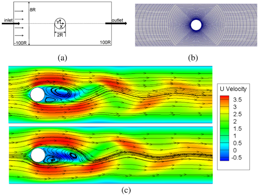
(a) Geometry, (b) mesh, and (c) typical streamlines for the simulation of unsteady viscoelastic flow past a cylinder.
Benchmark 2
Contraction flow
This is another typical benchmark flow problem in studying nonlinear dynamics of viscoelastic fluid. The 2D schematic diagram and computational mesh are presented in Figure 3(a) and (b) simulating the interesting nonlinear phenomena that polymer fluids in abrupt contraction flow exhibit. The mesh contains 42,472 cells and its density is graded from the interface and the horizontal centerline of the two channels. The deltaT for this case is set in the same way as in Cylinder Flow. The highly nonlinear phenomenon of viscoelasticity is shown in Figure 3(c) and the solver is also FENE-CD-JS.
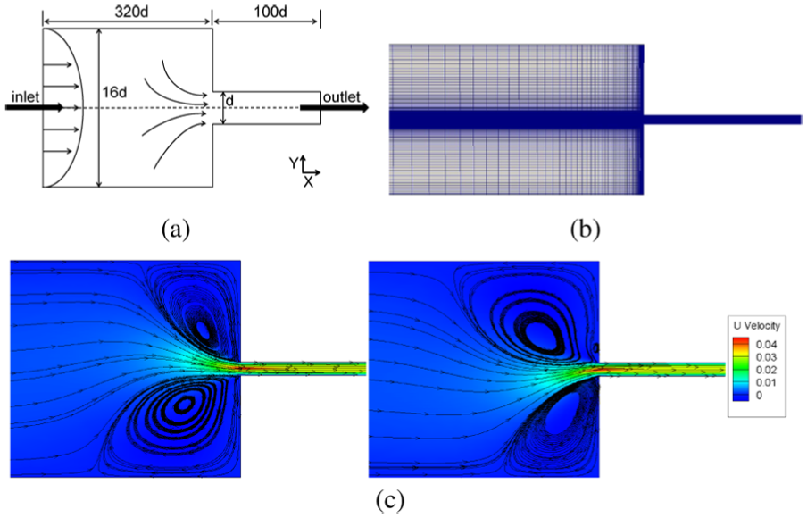
(a) Geometry, (b) mesh, and (c) streamline patterns for the 2D abrupt planar contraction flow.
Benchmark 3
MotorBike
This is a 3D steady-state simulation of motorbike and rider with Reynolds-averaged Navier–Stokes (RANS) k-omega shear stress transport (SST) flow model in OpenFOAM. The mesh consisting of 3,123,465 cells is generated by the snappyHexMesh tool. The initial flow condition is created with potentialFoam, and simpleFoam is adopted as the steady-state solver. The geometry and computational mesh can be seen in Figure 4(a) and (b). Since this is a steady-state simulation, the lengths of timesteps are generally much larger than those of transient simulations such as Cylinder Flow and Contraction Flow. The deltaT for this case is fixed as 1. Two streamline patterns during the simulation are plotted and presented in Figure 4(c) and (d).
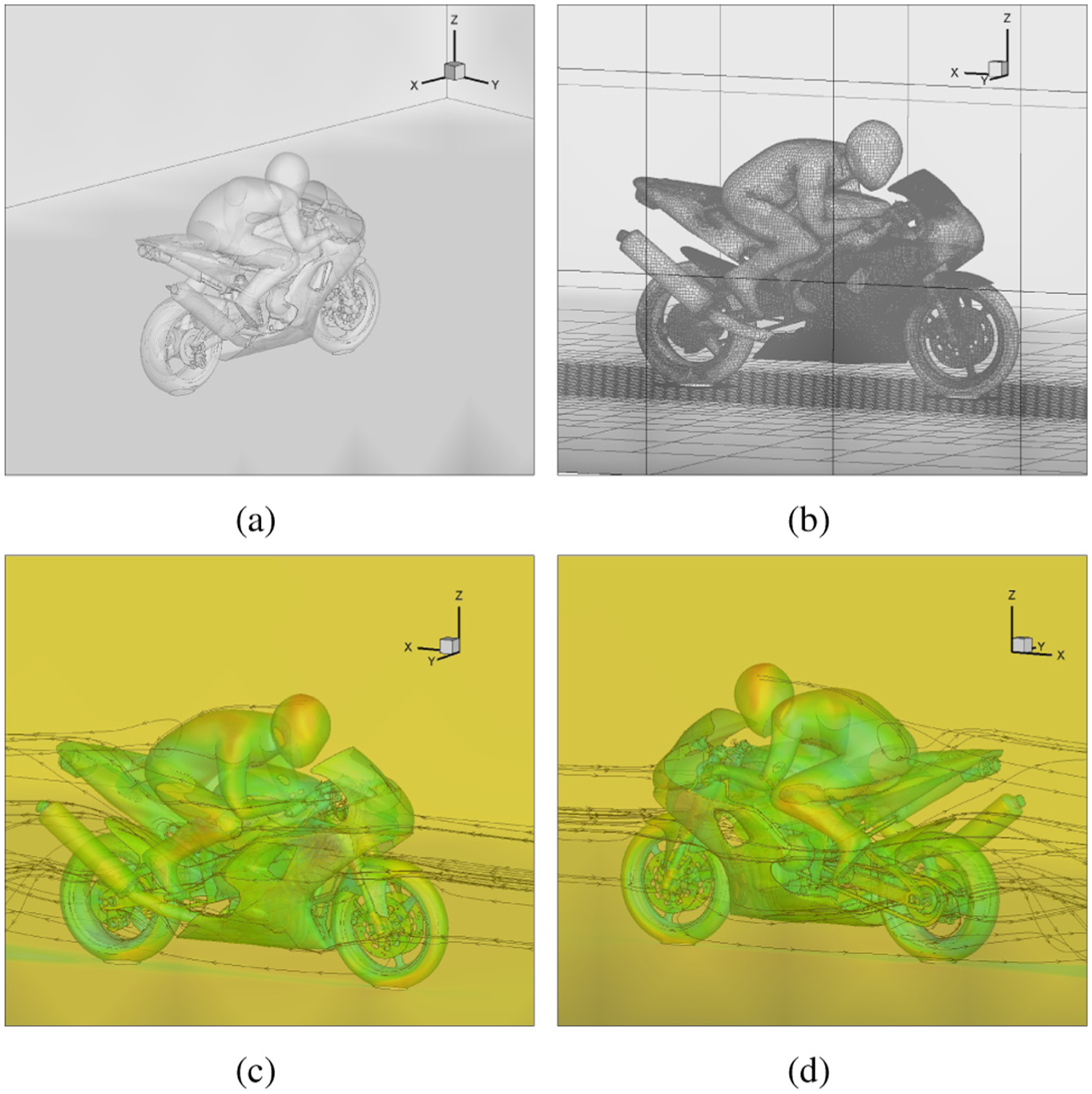
(a) Geometry, (b) mesh, and (c and d) streamline patterns for the 3D steady-state motorbike and rider simulation.
Benchmark 4
DamBreak
The feature of this problem is a transient flow of two fluids separated by a sharp interface. The setup consists of a column of water and the other fluid at rest located behind a membrane on the left side of a tank (see Figure 5(a)). At time = 0, the membrane is removed and the column of fluids collapses. During the collapse, the fluids impact an obstacle at the bottom of the tank and create a complicated flow structure, including several captured pockets of air. The mesh as shown in Figure 5(b) is unified containing 35,200 cube cells, that is, all the cells are cubes with the same size. The deltaT is initially set as 1e−6 and dynamically adjusted by Courant number during the simulation as well. The flow field changes drastically which can be seen in Figure 5(c) and (d). Solver for this case is interMixingFoam which is based on multiphase Volume-of-Fluid (VOF) method in OpenFOAM.

(a) Geometry, (b) unified mesh, and (c and d) computed volume fractions of air at two different timesteps during the simulation for the DamBreak simulation.
The four benchmarks we choose are quite representative. Both the first two ones are 2D mesh-graded, while the flow field of Cylinder Flow is quite steady and that of Contraction Flow asymmetrically oscillates a lot. Thus, we can examine whether using face areas to approximate matrix values is good enough for constructing an efficient parallel preconditioner. MotorBike is set up to examine the efficiency of FMetis in large-scale 3D simulations. DamBreak adopts an uniform mesh but exhibits more heterogeneous and complex flow field. Under this circumstance, FMetis goes back to OMetis since all the faces have the same area. From DamBreak, we would like to know whether FMetis still performs well comparing with MMetis which considers matrix values directly. Based on these four representative cases, the general performance of FMetis can be evaluated quite well.
Of all the four benchmarks, pressure implicit splitting of operators (PISO) algorithm 23 is adopted in which velocity equations and pressure equations are solved in a coupled way. The most time-consuming part of PISO algorithm lies in iteratively solving the large-scale linear systems derived from the pressure equation discretizations. The iterative solver is DIC-PCG in OpenFOAM, specifically, based on diagonal incomplete Cholesky factorization preconditioning.
Methodology
For each benchmark, we first focus on performances of different partitioning methods at the first timestep from time = 0. FMetis is compared with OMetis and MMetis(0). In all the three methods, the mesh is formulated by a corresponding adjacency graph. The major difference among the methods is how to assign the edge weights for the graph. The details of the three methods are introduced as follows:
FMetis. As we have introduced previously, FMetis partitions a mesh by partitioning its corresponding adjacency graph. Face areas are assigned to the graph edges as weights.
OMetis. In OMetis, there are no specific weights assigned to the edges of the graph. Considering that the partitioning is conducted by the original Metis method, we name it as OMetis.
MMetis(0). The matrix coefficients in the timestep from
All the three methods are based on the METIS_PartGraphRecursive routine but with different edge weights. Like the procedure illustrated in Algorithm 1, these weights are passed to the routine by the adjwgt parameter. After that the edge-weighted graph is partitioned by METIS_PartGraphRecursive. The METIS_PartGraphRecursive is chosen as its recursive bisection algorithm produces nearly perfect load balance. Accordingly, we can focus on evaluating the performances of the partitioning methods on the iterative convergence rate and the communication overhead, which are the two main factors affecting the overall parallel efficiency. Noting that the recursive algorithm is usually quite slow for large-scale problems and large number of partitions, faster partitioning routines might be more recommendable for this circumstance in real engineering applications.
Performance comparison for only one timestep is not enough to evaluate these partitioning methods. For each benchmark, we randomly choose a starting time and run the simulation for hundreds of timesteps. Performances of different partitioning methods along with the timesteps are compared. In this part, we compare FMetis with OMetis, MMetis(t1), and ParMetis. MMetis(t1) and ParMetis are introduced as follows.
MMetis(t1). MMetis(t1) is similar to MMetis(0), the only difference is that the matrix coefficients come from a different timestep. We pre-run the simulation in serial to
ParMetis. ParMetis supports dynamic mesh repartitioning.
24
It can be treated as a parallel version of Metis. Since the physical fields might change along with the timesteps, the best overall iterative convergence rates should be achieved by repartitioning the mesh every timestep with present matrix coefficients as edge weights. At the beginning of each timestep, the PDEs are not discretized yet. Thus, the matrix coefficients are not available. In every timestep (except for the first one), ParMetis utilizes the matrix coefficients from the previous timestep to repartition the mesh. How the matrix coefficients are used can be seen in Figure 6. Supposing the sample mesh at timestep t is distributed on two processors

(a) A sample distributed mesh and its corresponding graph and (b) the distributed matrix pattern from the previous timestep. The elements
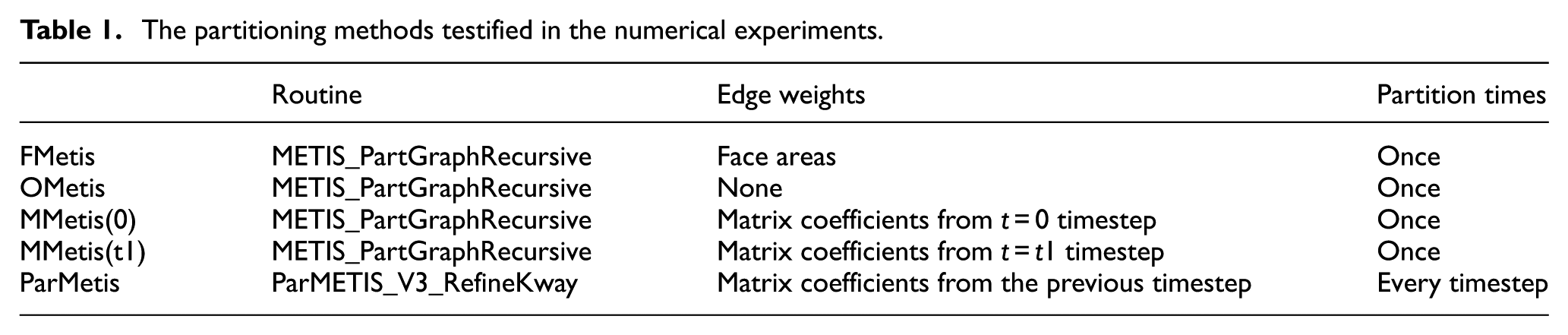
A brief summary of all the partitioning methods is presented in Table 1. It should be noticed that MMetis(0) and MMetis(t1) are established for comparison with FMetis. They are not quite practical in real CFD applications since users need to pre-run the simulation and record the matrix coefficients before mesh partitioning. We compare FMetis with MMetis since we want to know whether FMetis can approximate the matrix coefficients well with the face areas and produce partitions with good parallel preconditioners.
The partitioning methods testified in the numerical experiments.
The performance evaluation of all the partitioning methods includes comparison on LIB, total communication volume, maximum number of neighbor processors, number of iterations, and solving time of DIC-PCG. The time spent on preconditioning is already included in the solution time. Performance comparisons in our experiments only focus on several hundreds of iterations at most, thus the solution time may be only several hundreds of seconds. But notice that large-scale complex fluid flow problems are usually composed of hundreds of thousands of timesteps. The percentage of the performance improvement is significant and should be noticed.
Results and analysis
Performance comparison at t = 0 under different parallel degrees
The API routine of Metis requires a previously defined imbalance criterion which is 5% in our experiments. Thus, the partitioning heuristics only need to guarantee that the LIB be restricted within 5%. All the partitioning methods meet the load balancing requirement.
The total communication volumes (the total edge-cuts) of the partitioning methods are shown in Figure 7. As we know, not only the communication volume but also the communication frequency is significant to the communication overhead. The maximum numbers of neighbor processors under different numbers of processors are presented in Figure 8. For Cylinder Flow, Contraction Flow, and MotorBike, the total communication volumes (the total edge-cuts) of FMetis lie between those of OMetis and MMetis(0), for the reason that OMetis partitions the mesh using the total edge-cut as the cost function while MMetis(0) considers only about matrix values. FMetis is somehow a compromise between them. Performances of all the three methods in the maximum number of neighbor processors are similar to each other in most instances. In Contraction Flow with large numbers of processors, the maximum number of neighboring processors of MMetis(0) is significantly larger than those of OMetis and FMetis. In DamBreak, FMetis is equal to OMetis since all the faces are with the same area. There is no significant difference in the total communication volume from Figure 7(d). However, the maximum numbers of neighbor processors of FMetis and OMetis are smaller than that of MMetis(0) obviously from Figure 8(d).

Total edge-cuts of the three partitioning methods under different number of processors for (a) Cylinder Flow, (b) Contraction Flow, (c) MotorBike, and (d) DamBreak.

The maximum number of neighbor processors of the three partitioning methods under different number of processors for (a) Cylinder Flow, (b) Contraction Flow, (c) MotorBike, and (d) DamBreak.
Combining Figures 7 and 8, OMetis performs best in the communication overhead generally. FMetis is between OMetis and MMetis(0).
Considering the number of iterations of DIC-PCG at time = 0 under different partitions with various numbers of processors (Figure 9), for Cylinder Flow, Contraction Flow and MotorBike, no doubt that FMetis performs significantly better than OMetis and close to MMetis(0). For DamBreak, FMetis goes back to OMetis. The number of iterations under MMetis(0) is smaller than those under OMetis and FMetis.
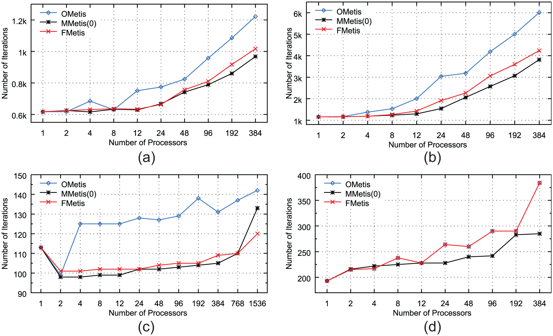
Numbers of iterations of DIC-PCG of the three partitioning methods at time = 0 under different number of processors for (a) Cylinder Flow, (b) Contraction Flow, (c) MotorBike, and (d) DamBreak.
In Cylinder Flow, Contraction Flow, and MotorBike, FMetis shows a competitive performance on DIC-PCG solving time and sometimes even better (Figures 10–12). The reason is likely to be that FMetis gives partitions with less communication overhead than MMetis(0). Especially under large numbers of processors in MotorBike, performance of MMetis(0) becomes the poorest because of its large communication overhead. Mostly, the DIC-PCG time of OMetis is the largest of all the partitioning methods in Cylinder Flow and Contraction Flow. In DamBreak as shown in Figure 13, MMetis(0) outperforms the other partitioning methods a little due to its best performance in the iterative convergence rate.

Normalized DIC-PCG solution time of the three partitioning methods to the time of OMetis at time = 0 under different number of processors for Cylinder Flow.

Normalized DIC-PCG solution time of the three partitioning methods to the time of OMetis at time = 0 under different number of processors for Contraction Flow.

Normalized DIC-PCG solution time of the three partitioning methods to the time of OMetis at time = 0 under different number of processors for MotorBike.

Normalized DIC-PCG solution time of the three partitioning methods to the time of OMetis at time = 0 under different number of processors for DamBreak.
Performance comparison at t = 0 under optimal parallel degrees
To assess FMetis clearly, statistics for the four cases under their optimal parallel degrees (96, 24, 768, and 48) are listed in Tables 2–5, respectively. The statistics include the LIB, the total edge-cut, the maximum number of neighbor processors (Max NNeiProcs), the number of DIC-PCG iterations (NIterations), and the solving time of DIC-PCG (IterTime).
Cylinder Flow: performance comparison under the number of processors 96 at time = 0.

LIB: load imbalance.
Contraction Flow: performance comparison under the number of processors 24 at time = 0.

LIB: load imbalance.
MotorBike: performance comparison under the number of processors 768 at time = 0.

LIB: load imbalance.
DamBreak: performance comparison under the number of processors 48 at time = 0.

LIB: load imbalance.
From the Tables 2–5, we can get that MMetis(0) always performs best except in MotorBike. It is reasonable that MMetis(0) performs best in a simpler case. The weights for MMetis(0) are from the linear system of the timestep from time = 0. Using the linear system information that we are solving for, it makes sense that we can get a better partition than using face areas. But in MotorBike, MMetis(0) produces a large amount of communication overhead. Therefore, the solving time is quite large even though the number of iterations is quite low. FMetis shows 14.34%, 23.34%, and 19.44% performance improvement in the DIC-PCG solving time than OMetis in the first three cases, respectively. In DamBreak, FMetis goes back to OMetis.
Performance comparison at different timesteps under optimal parallel degrees
To testify the robustness of FMetis, in other words, to verify whether partitions produced by FMetis can perform well during the whole simulation, we choose a starting time point for each benchmark and run the simulation for some time to observe FMetis’s performance. In this section, not only the iterative convergence rate and DIC-PCG solving time are recorded, but also the repartitioning overhead that ParMetis introduces and the overall simulation time accumulated along with the simulations.
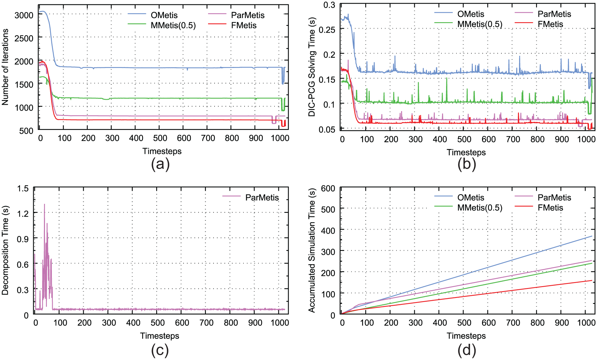
Results for Cylinder Flow from time = 0 is shown in Figure 14. FMetis shows a performance a little better than MMetis(0.3). Both of them perform better than ParMetis after several timesteps from the beginning of the simulation. We look deep into the partitioning algorithm of ParMetis and speculate the main reason to be that the parallel partitioning heuristic may have the problem of low efficiency and local optimum. If the matrix pattern does not change much between neighboring timesteps, it is not easy for ParMetis to recalculate a better partition. However, since FMetis considers the static components of the linear systems, it can achieve a general good performance as the simulation goes. In addition, ParMetis introduces a lot of additional overhead on repartitioning which makes the overall simulation time much longer than other partitioning heuristics.

Cylinder Flow, number of processors 96, from time = 0: (a) number of iterations, (b) parallel DIC-PCG solution time, (c) time spent on repartitioning for each timestep, and (d) the total simulation time including mesh repartition, field redistribution, PDE discretization, and solving linear systems accumulated with the timesteps.
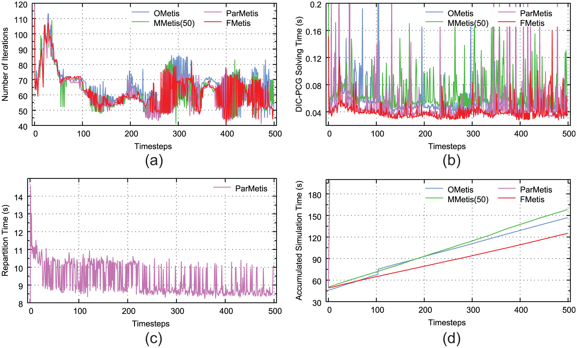
For Contraction Flow, the results from time = 0.5 are listed in Figure 15. In this benchmark, FMetis performs best of all the partitioning methods, especially after about 80 timesteps from the beginning. Although the linear system patterns may change a lot during the simulation, FMetis succeeds in capturing the most important and static component which makes it maintain a good performance all along the simulation.
Contraction Flow, number of processors 24, from time = 0.5. (a) Number of iterations, (b) parallel DIC-PCG solution time, (c) time spent on repartitioning for each timestep, and (d) the total simulation time including mesh repartition, field redistribution, PDE discretization, and solving linear systems accumulated with the timesteps.
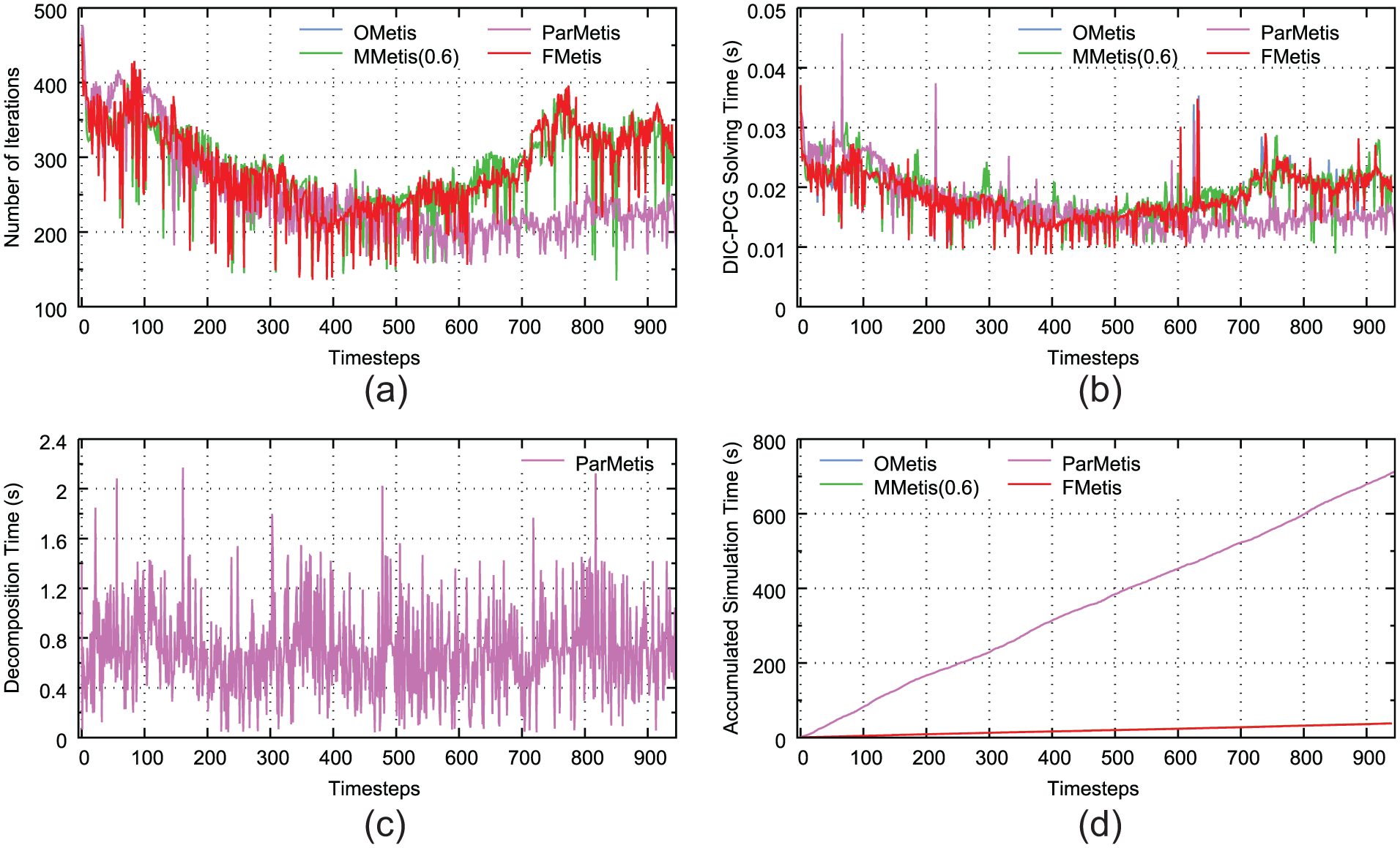
As shown in Figure 16, FMetis exhibits the best performance generally in MotorBike. ParMetis is not able to produce the best iterative convergence rate throughout the simulation. Notice that for such a large-scale 3D simulation, the repartitioning overhead of ParMetis is quite large as shown in Figure 16(c). The total simulation time using ParMetis is 6619.66 s which is not available in Figure 16(d). Every time the mesh is repartitioned, related cells and various physical fields need to be transferred among processors. This procedure causes significant overhead for complex CFD applications. Thus, we suggest a good static partitioning method or working on better repartitioning schemes for iterative convergence feature.
MotorBike, number of processors 768, from time = 0. (a) Number of iterations, (b) parallel DIC-PCG solution time, (c) time spent on repartitioning for each timestep, and (d) the total simulation time including mesh repartition, field redistribution, PDE discretization, and solving linear systems accumulated with the timesteps.
In DamBreak, the results from time = 1.05 are listed in Figure 17. By repartitioning the mesh every timestep, ParMetis exhibits better performance in the number of iterations and DIC-PCG solving time after about 700–800 timesteps. The other partitioning heuristics perform similarly with each other. As we have mentioned above, the flow phenomenon changes dramatically along with the timesteps, thus ParMetis is able to adjust its partition every timestep and improve the iterative convergence feature. The cost is a large amount of additional repartitioning overhead. For this kind of problem, a good choice should be repartitioning the mesh only when needed. Working out suitable repartitioning chances to obtain a trade-off between the solution time and repartitioning time needs further research which is beyond the scope of this article.
DamBreak, number of processors 48, from time = 1.05. (a) Number of iterations, (b) parallel DIC-PCG solution time, (c) time spent on repartitioning for each timestep, and (d) the total simulation time including mesh repartition, field redistribution, PDE discretization, and solving linear systems accumulated with the timesteps.
On the basis of our numerical results, we can see that FMetis performs much better than OMetis in CFD applications with non-uniform generated mesh. Comparing with MMetis series methods, FMetis has a similar performance and sometimes can be even better. It captures the core factor that influences the magnitudes of matrix coefficients and generates good partitions for the overall simulation. While for uniform mesh, FMetis goes back to OMetis. Under this circumstance, appropriate dynamically repartitioning heuristic is needed in further study. In addition, since FMetis is based on the mesh topology information, its partitioning time is similar to OMetis which makes it efficient and easy to use.
Conclusion
We construct approximations of matrix off-diagonal entries on mesh topology for better iterative convergence rate in parallel CFD simulations. Considering FVM-based problems, face area is theoretically proved to be a suitable approximation and a new partitioning heuristic is formulated and implemented as FMetis. FMetis is general, fast, and easy to use since it is absolutely based on the mesh topology which is crucial in practice. Numerical results on four CFD applications indicate that FMetis performs noticeably better than the traditional standard partitioning method for non-uniform meshes. As the simulation goes, the flow field might change a lot. The most significant advantage of FMetis is its stable performance improvement along with the timesteps. Partitions produced by FMetis always show good preconditioning quality and the overall efficiency can be significantly improved.
Footnotes
Acknowledgements
The authors thank State Key Laboratory of High Performance Computing for providing the facilities to support the research.
Handling Editor: Jose Ramon Serrano
Declaration of conflicting interests
The author(s) declared no potential conflicts of interest with respect to the research, authorship, and/or publication of this article.
Funding
The author(s) disclosed receipt of the following financial support for the research, authorship, and/or publication of this article: This research is funded by National Key Research and Development Program of China (2016YFB0201301), Science Challenge Project (JCKY2016212A502), and the open fund from the State Key Laboratory of High Performance Computing (201503-01 and 201503-02).