
Abstract
The impact of fluid on the runner of a hydraulic turbine is a recurrent problem. Fully coupled fluid–structure simulations are extremely time-consuming. Thus, an alternative method is required to estimate this interaction to perform a reliable rotor dynamic analysis. In this article, numerical estimations of the added inertia, damping, and stiffness for a Kaplan turbine model runner are presented using transient flow simulations. A single-degree-of-freedom model was assumed for the fluid–runner interaction, and the parameters were estimated by applying a harmonic disturbance to the angular velocity of the runner. The results demonstrate that the added inertia and damping are important, whereas the stiffness is negligible. The dimensionless added polar inertia is 23%–27% of the reference value
Introduction
Hydraulic turbines are typically refurbished approximately every 40 years. A refurbishment typically involves new parts, such as the runner, guide vanes, bearings, and generator, whereas the water ways are unmodified mainly due to the high cost of replacing these components. To increase the power output of a hydraulic turbine in addition to improving the efficiency, the runner hub diameter is decreased to make a larger amount of water move through the turbine. The runners are also becoming lighter because of advancements in materials technology. Developments in numerical simulations and model testing have enabled the design and installation of more efficient runners. The changes in design alter the dynamics of the system, and a rotor dynamic analysis must therefore be performed to determine the natural frequencies of the system to avoid potential resonance during operation. The effect of the surrounding water, which adds mass, damping, and stiffness to the system, is important for the rotor dynamic analysis.
The added mass determines the kinetic energy that is transferred from the structure motion to the fluid. 1 In other words, the added mass or apparent mass is defined as a part of the surrounding fluid accelerated by the movement of the structure with respect to the fluid. 2 The added damping, which reduces the vibration amplitude, is mainly expressed by the dissipated structural energy. For example, the bulk of the energy is expended on generating the trailing edge vortices for a runner blade, which can be considered as an unsteady lifting surface. 3 The last added parameter, called the added stiffness, is similar to the added damping and depends on the motion of the structure and surrounding flow. 4
Due to recent technological advancements and increased computational capacity, computational fluid dynamics (CFD) can now be used to analyze the fluid–structure interaction. In addition to the stiffness and damping, the added mass has been studied for simple objects 5 and complex structures, such as pumps6,7 and off-shore structures. 8
Liang et al. 9 investigated the fluid–structure interaction of a Francis turbine runner with the finite element method to determine the dynamic coefficients in still water and air. The effect of added inertia was studied by considering the natural frequency, frequency reduction, and mode shapes under both conditions. A comparison of the results can help to determine the influence of surrounding water on the natural frequencies, damping ratio, and added inertia. The results for the natural frequencies and mode shapes were consistent with those of earlier experiments. 10
Structural analysis with CFD was also performed for Francis and Pelton runners. 11 These investigations9–12 focused on the vibration and mode shapes of the runner instead of the dynamic properties of the entire rotor system. Researchers have devoted considerable effort to investigating Francis turbines,9,12–15 whereas Kaplan turbines have received less attention. The deflection of the Kaplan turbine runner for different Young’s moduli was simulated using one-way and two-way coupled fluid–structure interactions. 16 De Souza Braga et al. 17 performed a modal analysis and an experimental investigation of a Kaplan turbine runner. The mode shapes and natural frequencies of the runner in still water and air were presented and compared.
The rotor dynamic coefficients of hydraulic machines, for example, Francis and Kaplan turbines, are leading parameters that have not been comprehensively identified. An experimental study of the effect of the surrounding water on the hydraulic machines is extremely challenging due to the size and complex experimental implementation. Numerical and analytical methods are useful for gaining insight into the fluid and structure interactions while avoiding experimental difficulties. Karlsson et al. 18 studied the added polar inertia and damping of a Kaplan turbine model at three different operating points via CFD. Only four points were evaluated at high perturbation frequencies, which were at least 10 times larger than the rotational frequency of the runner. The added polar inertia decreased, and the added damping increased with increases in the perturbation frequency at the off-design operating points. Both added properties increased at the best efficiency point (BEP). Both high and low excitation frequencies are of interest for Kaplan turbines, for example, the rotating vortex rope frequency is 0.2–0.4 times the runner frequency.
Keto-Tokoi et al. 19 presented an analytical method based on Theodorsen’s unsteady thin-airfoil theory to quantify the added mass and damping of various Kaplan runners. The results from the finite element (FE) simulation and the analytical method were compared. The added mass increased with increases in the number of blades and runner diameter. Puolakka et al. 20 used the same analytical method to examine three Kaplan runners with variations in several characteristics, such as the blade number, specific speed, tip clearance, and hub ratio. The added mass and damping in the polar, axial, and polar–axial directions for the runners were compared with the FE simulations. An increase in added mass in the polar, axial, and polar-axial coordinates was observed in the studied frequency range. However, the added damping tended to decrease with increases in frequency. A similar method, namely, two-dimensional (2D) thin-airfoil theory with lifting-line theory, was used to determine the added mass and damping of a marine propeller. 21
The available literature on the influence of runner rotation and the associated rotating flow field on the fluid-added properties for torsional vibration is limited. 19 Both numerical and experimental modal analyses, which are used to determine the effect of the added mass, are intended for stationary objects. Therefore, a computational tool that considers the effect of the rotation, turbulence, and flow unsteadiness would be useful. In this work, a wide range of perturbation frequencies was investigated using transient CFD for a Kaplan turbine model.
This article presents the fluid-added properties for the runner of a Kaplan turbine model. The runner is assumed to be rigid, and the main objective is to identify the added properties that result from the fluid interaction. Then, these properties can be used in a rotor dynamic analysis of the entire rotor system. The runner operates at a constant rotational speed subjected to perturbation frequency, and 20 different perturbation frequencies were considered here. This study considers a wider range of perturbation frequencies than the study of Karlsson. 18 This study considers frequencies that are 0.5–10.1 times the runner operating frequency. An analysis method was developed with least squares fitting to determine all the coefficients. The results are presented as frequency-dependent coefficients.
Numerical simulation
The Kaplan model investigated in this work is known as the Porjus U9 model. The fluid part has been experimentally and numerically investigated in detail by Mulu and colleagues22–24, Jonsson et al. 25 and Amiri et al.26–28 This model is a 1:3.1 scale of the 10 MW prototype turbine, which has a runner diameter of 1550 mm. The turbine is composed of 18 unequally distributed stay vanes, 20 guide vanes, and 6 runner blades. The model runner has a diameter of 500 mm, and its hub-to-tip ratio is 0.52. The runner shroud and tip solidity are 0.87 and 1.2, respectively.
The computational model used in this study is presented in Figure 1, which was extracted from the numerical simulations of Mulu et al. 24 The spiral casing and stay vanes are omitted because their presence is not required to capture the flow near the runner.

Computational domain comprising the guide vanes, runner, and draft tube.
As shown in Figure 1, the complete geometry of the guide vanes and runner was used for the simulation. The computational domain includes three domains, which are connected to one another with general grid interfaces (GGIs). The mesh used in the simulations was selected based on the mesh study of Mulu et al. 24 Hexahedral-type elements were used for all parts, including the guide vanes, runner, and draft tube. The mesh resolution at the hub clearance and tip clearance is shown in Figure 2. The number of cells in both regions was 5–10. The total number of elements in this study was approximately 17 million. A 2D view of the mesh at the mid-span of the runner blade is shown in Figure 3.
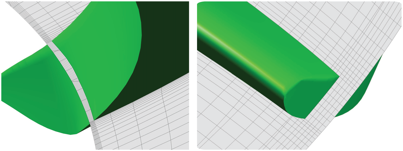
Mesh density at the hub clearance near the trailing edge (left) and the tip clearance near the leading edge (right). The blade is shown in green.

Blade-to-blade view of the inter-blade channel mesh at the mid-span of the runner blade.
The simulations were performed at the BEP for the U9 model. The operating parameters are presented in Table 1.
Operational condition parameters for the U9 model.

In this study, the unsteady Reynolds-averaged Navier–Stokes approach was applied to perform the simulations using the commercial software ANSYS CFX 16.2. This software uses an element-based finite volume method that implements various discretization schemes. The high-resolution discretization scheme was applied for the continuity and momentum equation advection term. Using a blend factor parameter, this scheme can perform the first-order upwind in a high-gradient region or the second-order scheme in a low-gradient region. 29 The first-order upwind scheme was used for the advection terms in the turbulence equations. This solver is pressure-based and coupled, that is, the continuity and momentum equations are solved in a fully coupling manner. The mass flow was discretized in a manner similar to that suggested by Majumdar, 30 who presented a modified version of the Rhie and Chow’s 31 discretization. The simulations require a sufficiently small time step to resolve various phenomena in the flow. The time step was set to 3.6e−4 s, which corresponds to approximately 1.5° of the runner revolution. The simulations were run until a periodic flow was achieved at specific monitor points. After reaching convergence, the data were recorded for evaluation in the present investigation.
According to the numerical simulation of Mulu et al., 24 who investigated many turbulence models (k−ε, re-normalisation group (RNG) k−ε, shear stress transport (SST) and scale-adaptive simulation–shear stress transport (SAS-SST)) to simulate the Porjus U9 model at the BEP, the standard k−ε model with a scalable wall function is suitable and was used to perform the simulations. A scalable wall function can handle fine meshes near the wall regardless of the Reynolds number. 29 To consider the transient flow characteristics, a transient rotor–stator interface was selected as the domain interface between the rotating and stationary domains. A sliding interface was used between the domains to resolve the transient interactions. This model is highly cost-effective because it includes all transient features.
Modeling of the system
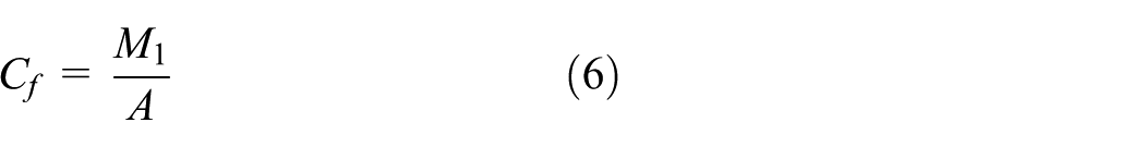
The runner of the Kaplan turbine is modeled as a rigid disk to formulate the torsional vibration with 1 degree of freedom. The equation that governs the forced torsional vibration with a single degree of freedom is

where
We assume that the unsteady perturbations induced by different sources can be characterized by a harmonic perturbation with constant amplitude and frequency. To investigate the added properties, a prescribed harmonic perturbation

where
A total of 21 transient simulations were performed for the following values of the perturbation frequency factor k: 0.5, 1, 1.5, 2, 2.5, 2.9, 3, 3.01, 3.1, 3.5, 4, 4.5, 5, 5.5, 6, 7, 8, 9, 9.9, 10, and 10.1. The perturbation frequency factors used were spaced at intervals of 0.5 from 0.5 to 5.5 and at intervals of 1 from 6 to 10; five additional values were also included: 2.9, 3.01, 3.1, 9.9, and 10.1. Due to these harmonic disturbances, an additional moment

We assume that the additional torsional moment of the turbine takes the following form

where

The added damping is independent of the added inertia and stiffness. Because the added inertia and stiffness appear in the same equation, an assumption is required to solve the set of equations. According to a previous study, 10 the effect of the added stiffness is negligible for a Francis turbine runner. In other studies, the right-hand side of equation (5) is expressed using only a frequency-dependent added inertia to obtain the added mass of the Kaplan runner. 20 The added inertia and damping can be calculated directly without considering the added stiffness in the set of equations.
A simple method to obtain the added polar inertia is to define it to be constant over the operational range. According to equation (5), if the second-order polynomial is fit on the right-hand side of the equation, the added polar inertia can be easily obtained as approximately 0.277 (Figure 4).
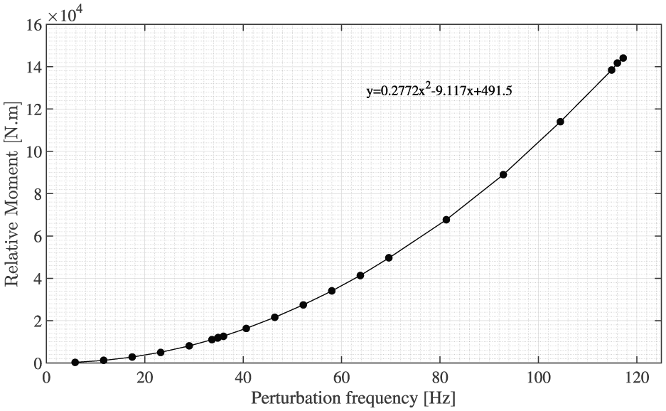
Right-hand side of equation (5) as a function of the perturbation frequency.
In addition to the aforementioned method, an approach is proposed to investigate the supposedly negligible effect of the added stiffness. In this approach, the added mass and stiffness are defined to be constant over a frequency interval
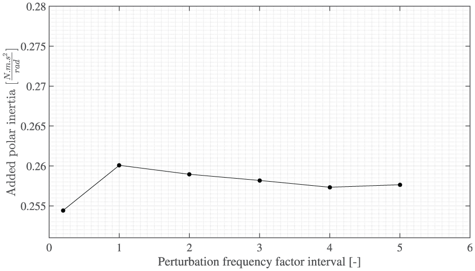
Polar inertia sensitivity analysis for the perturbation frequency factor interval.
Fluid simulations were performed for various perturbation frequencies to obtain the moment. Then, the parameters were calculated using the zero-stiffness definition and developed method.
Results
The simulations were performed with ANSYS CFX, and the total moment was extracted for the vibrational analysis. Figure 6 shows the total moment and rotational speed of the turbine. In this case, the perturbation frequency is five times the runner frequency.

Moment and angular velocity for
Figure 6 shows a phase shift between the angular velocity and moment. As described in equations (5) and (6), the phase shift plays a key role in the estimation of fluid-added properties. The phase shift between the forced rotational speed and obtained moment is shown in Figure 7 with respect to the perturbation frequency. With increasing perturbation frequency, the phase shift increases to approximately 65°, which indicates that the forced rotational speed and moment maintain a nearly constant phase shift at higher frequencies greater than 40 Hz. Therefore, the added properties depend more on the moment amplitude than on the phase shift at higher perturbation frequencies. A maximum value of 70° occurs at 70 Hz, which corresponds to a frequency factor of 6.

Phase shift as a function of the perturbation frequency.
The last two periods are used to obtain the fitted curve, and the phase and amplitude of the moment can be solved. The moment function is estimated to a harmonic signal using the least squares method in MATLAB. The curve fitted to the moment is presented with the input in Figure 8.
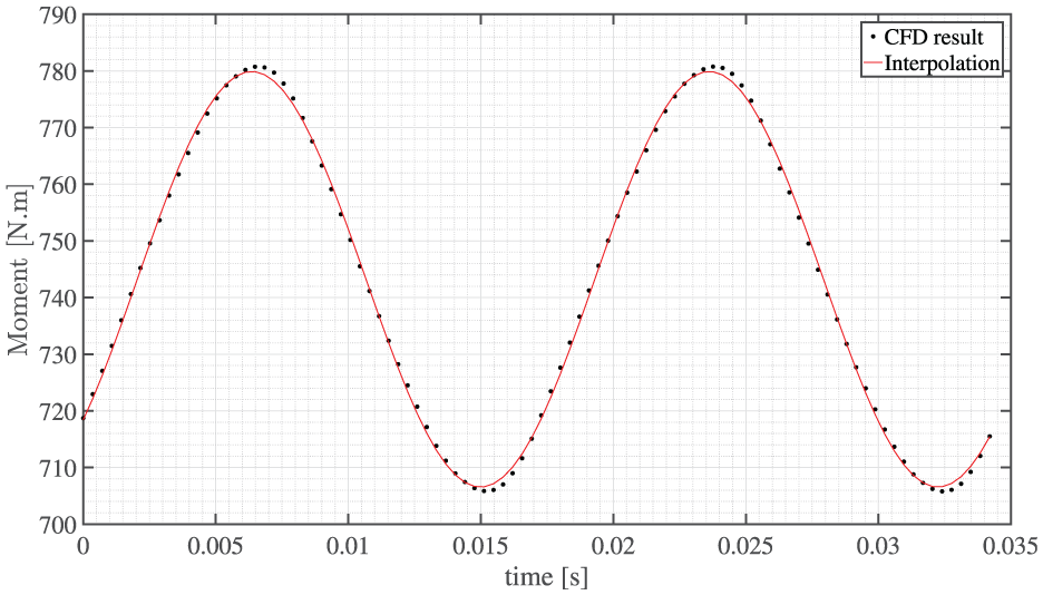
Moment and least squares fitted curve for
The moment is not a single harmonic function, which indicates that the problem is nonlinear. At lower frequencies, the deviation decreases, and the system is linear, as shown in Figure 8. However, an error in the estimation of added properties is expected at higher perturbation frequencies because of the nonlinearity and the inaccuracy of the curve-fitting.
Two methods for estimating the added properties, which are used in this study, are briefly described below:
The added inertia and damping can be estimated at various perturbation frequencies by defining the added stiffness as zero. If any added stiffness effectively exists due to the presence of the flow, the estimated added inertia value will be underestimated with such assumption according to equation (5) (Figure 9).
In the other method, the stiffness contribution is considered in the equations. The influence of the rotor dynamic parameters is defined as constant within a small perturbation frequency interval. Hence, the parameters are estimated by comparing the data in an interval
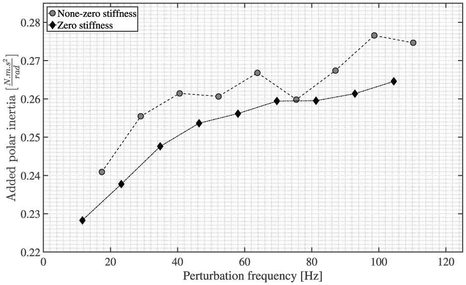
Added polar inertia as a function of the perturbation frequency.
Although the change in the parameters is not negligible in the selected perturbation frequency interval, the estimation error is low. The total error is higher when the perturbation frequency factors are closer together, for example, 2.9, 3.01, and 3.1 or 9.9 and 10.1, due to the higher numerical errors. Therefore, the aforementioned simulations are not considered in the subsequent analysis.
In Figure 9, the estimated polar inertia is shown and compared with the zero-stiffness solution (solid line). If a zero-added stiffness is assumed to determine the added inertia, the added stiffness resulting from the flow will influence the estimated value of the added inertia

where
Figure 10 presents the added damping as a function of the perturbation frequency. As illustrated in Figure 9, the added polar inertia increases more at the lower perturbation frequencies than at higher ones when assuming a stiffness of zero; conversely, the added damping is constant at perturbation frequencies below 35 Hz and increases at higher frequencies. The stiffness is shown as a function of the perturbation frequency in Figure 11.
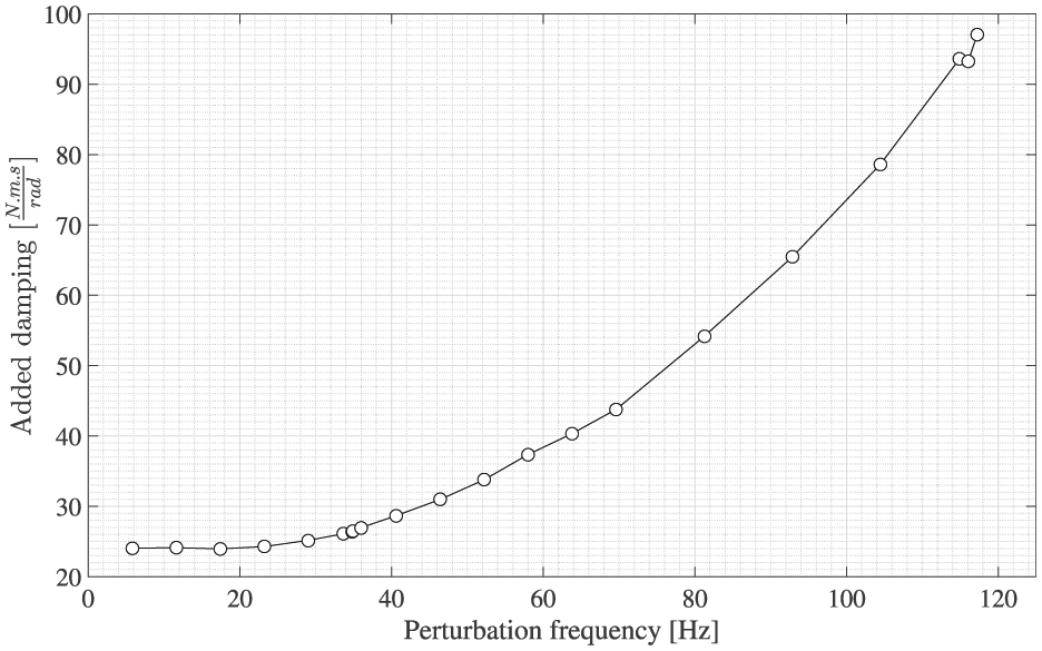
Added damping as a function of the perturbation frequency.
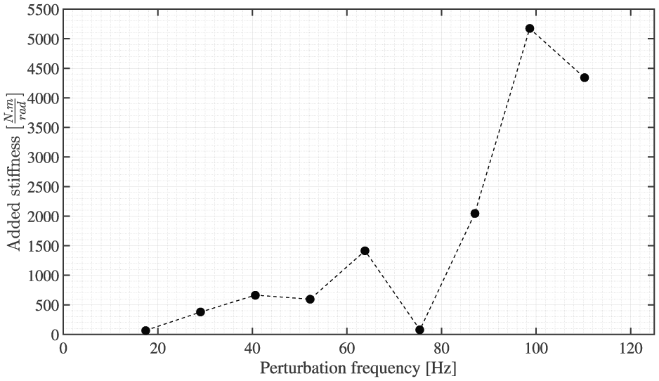
Added stiffness as a function of the perturbation frequency.
Following the zero-stiffness method presented above, the obtained added polar and damping are compared with the results of the study of Puolakka et al.
20
and Karlsson et al.
18
in Figures 12 and 13. The added properties are presented in dimensionless form using the reference values of

Dimensionless added polar inertia as a function of the perturbation frequency.
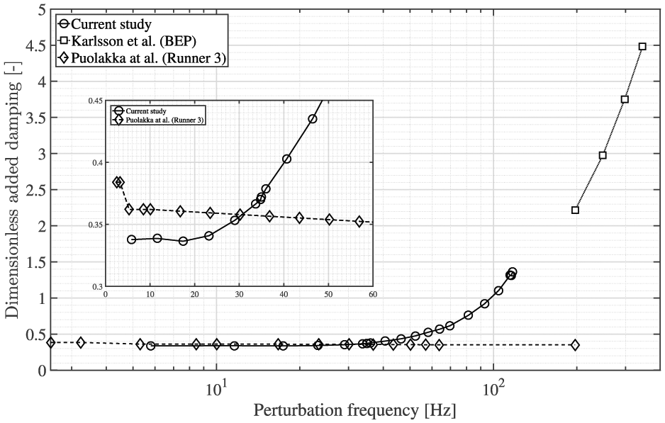
Dimensionless added damping as a function of the perturbation frequency.
The obtained added damping increases with the perturbation frequency. The results of the study of Karlsson et al. 18 have a similar trend but appear at higher perturbation frequencies. Nonetheless, both our results and those of Karlsson et al. have a similar overall trend. The magnitude of the added damping is in good agreement with the findings of Puolakka et al. 20 at lower frequencies (5–70 Hz) but not at higher perturbation frequencies (>70 Hz). As the operating conditions and geometry of the turbines in these two studies differ from those in our case, differences in the results are expected.
A comparison of the effect of each parameter in terms of its relative contribution to the additional moment indicates the significance of each. Figure 14 illustrates the relative contribution of the added polar inertia

Relative contributions of the polar inertia, damping, and stiffness to the additional moment.
As noted above, similar to Francis turbines, the added stiffness does not play a significant role in the Kaplan turbine rotor dynamics, as confirmed by its contribution to the total moment (Figure 14) compared to the added polar inertia and damping.
The blade inflow condition significantly affects the turbine performance and flow structure. For a given guide vane and runner blade angle, a different rotational speed of the turbine runner results in a different angle of attack and a different blade-relative velocity magnitude. Therefore, the time-dependent rotational speed imposed in the simulation is expected to induce a time-varying flow. The transient results with and without a perturbation are compared to identify any difference in the magnitude of the flow velocity in the inter-blade channel. Figure 15 illustrates the blade-to-blade velocity contour of the cases with and without perturbation at the mid-span. The velocity contour of the case with prescribed perturbation is presented at three phases: mean value, peak value, and base value of the perturbation amplitude. The perturbation frequency is 81.3 Hz.

Blade-to-blade velocity contour of the case with no perturbation (top left), mean value of the perturbation amplitude (top right), peak value of the perturbation amplitude (bottom left), and base value of the perturbation amplitude (bottom right).
The velocity contour remains qualitatively unchanged with and without imposed perturbation. A small difference is observed for the maximum flow velocity, which occurs on the suction side of the runner blade, between the cases without perturbation and with maximal perturbation amplitude. This small velocity variation does not change the flow field. Vortex shedding behind the runner blade was not observed due to either the high flow velocity and optimal blade angle at the BEP, which force the flow to attach to the blade and leave it smoothly, or/and the grid size, which is not sufficiently fine behind the runner blade to capture the vortex shedding. Further grid refinement to capture the vortex shedding would increase the computational complexity of the analysis considerably.
Discussion and conclusion
An alternative method to more accurately determine rotor dynamic parameters is desired in the design of hydro turbines. These parameters are important and must be included in the dynamic analysis of hydropower rotors. Recent developments in computational resources, CFD codes, and turbulence modeling have replaced the “rules of thumb” factors for determining the impact of added mass with more accurate estimations. 32 In this study, numerical simulations for various perturbation frequencies have been performed to estimate the added polar inertia, damping, and stiffness of a Kaplan turbine model runner. A single-degree-of-freedom model was assumed for the fluid–runner interaction, and the added properties were estimated by applying a harmonic perturbation in the angular velocity. The resulting moment from the simulations was assumed to be harmonic. This assumption was shown to give a good approximation at low perturbation frequencies, whereas the error in the assumed harmonic moment increased at higher frequencies because of nonlinear effects.
In general, all added properties increase with the excitation frequency in the studied range. In addition, nonlinear effects appear at high perturbation frequencies (greater than 40 Hz), as shown in Figure 8, which causes the uncertainty in the determination of the added proprieties. Furthermore, the parameter analysis indicates that added stiffness is negligible in the model; thus, the simplified estimation with zero stiffness is applicable. Comparisons with the reference polar inertia of the runner show that the fluid will add 23%–27% more inertia depending on the excitation frequency. The deviation from previous studies may be caused by the different flow rate, head, and geometry. Therefore, similar cases should be investigated to validate the results.
Footnotes
Acknowledgements
Handling Editor: Nima Vaziri
Declaration of conflicting interests
The author(s) declared no potential conflicts of interest with respect to the research, authorship, and/or publication of this article.
Funding
The author(s) received no financial support for the research, authorship, and/or publication of this article.