Sage Journals: Discover world-class research

Abstract

In most of the previous fault diagnostic literatures, the fault modes and states are pre-determined (i.e. the model structure (topology) is a priori known). However, in practical situation, the monitoring data, especially for the entire life-cycle data, nothing is known about the nature and the origin of the degradation (i.e. the model structure is unknown). Moreover, there is no consensus, how to determine the optimal model structure. In this condition, the different model structures may lead to different fault diagnosis/prognosis results. To address the optimal structure–selection problem, this article presents an automatic segmentation method based on Laplacian eigenmaps manifold learning and adaptive spectral clustering algorithms. Given an entire lifetime data of turbofan engine, we attempt to automatically segment the data into a sequence of contiguous regions corresponding to the degradation states. Furthermore, intrinsic dimensionality estimation, nonlinear dimension reduction, and the optimal number of degradation state estimation have been implemented. Automatic segmentation is applied for degradation state segmentation of non-label life-cycle data, and the output can be considered as the available information for developing fault diagnosis/prognosis. The experimental verification results indicate that the proposed automatic segmentation method is highly efficient and feasible for automatically determining the optimal model structure.

Keywords

Turbofan engine automatic segmentation fault diagnosis fault prognosis Laplacian eigenmaps adaptive spectral clustering

Introduction

The turbofan engine providing thrust to the aircraft is one of the most vital systems to aviation system, and large amounts of researches have been carried out in the area of turbofan engine fault diagnosis/prognosis.^1–5 The performance of an aircraft’s engine deteriorates when it is operated because its components physically degrade. To comprehensively describe the failure evolution, the degradation states before failure should be paid more attention.

So far, many available fault diagnostic techniques, such as kernel principal component analysis (PCA),⁶ Kalman filters,^7–9 sliding mode observer,¹⁰ support vector data description,¹¹ Bayesian network,¹² artificial neural networks,¹³ and hidden Markov model¹⁴, have been successfully applied in many industries. In most of these approaches,^15,16 it is assumed that the model structure is pre-determined, ignoring the basic segmentation problem: given an entire lifetime data, we wish to partition our data into contiguous regions corresponding to the degradation states (see Figure 1). The segmentation problem is taken into account in a few of these approaches with unsupervised clustering algorithms,^17,18 but the degradation state number is pre-determined as well. There are three possible reasons that explain why the degradation states division is rarely considered in the previous literatures: (1) the degradation states division process itself is time-consuming, (2) finding a reasonable degradation state structure which requires large amount of data, is usually not available in real world, and (3) the curses of dimensionality in high-dimensional data are still the major issue that challenges the degradation states division. Actually, the degradation states division is an important step for fault diagnosis and prognosis. If the number of degradation state is too small, the diagnosis/prognosis results are affected. On the contrary, the CPU time is expensive.

Figure 1.

Basic segmentation problem of lifetime data.

As a matter of fact, the life-cycle data of turbofan engine are the nonlinear and non-stationary time series, which contain abundant potential failure information. However, with the exponential increase of performance monitoring data, the curses of dimensionality are also the main issue that affects the accuracy of fault diagnosis/prognosis. Fortunately, manifold learning algorithm is a perfect tool for data mining that discovers the structure of high-dimensional data and provides better understanding of data.¹⁹ Recently, a variety of nonlinear dimensionality reduction techniques have been proposed which aim to address the limitations of traditional techniques such as PCA.²⁰ The core idea of manifold learning algorithm is to find a nonlinear low-dimensional embedding of high-dimensional data without losing much information. Additionally, the dimension of the embedding is a key parameter for manifold projection methods: if the dimension is too small, important data features are “collapsed” in the same dimension. On the contrary, the projections become noisy and unstable.²¹ There is no consensus, however, on how this dimension should be determined.

Automatic segmentation methods have been employed in image processing and speech recognition^22–24 but few about fault diagnosis and prognosis. Forecasting the future states of a complex system is a complicated challenge that is encountered in many industrial applications covered in the community of prognostics and health management. Practically, states can be either continuous or discrete: continuous states generally represent the value of a signal, while discrete states generally depict functioning modes reflecting the current degradation.^25–27 In this article, we introduce an automatic segmentation method which aims to address the optimal structure–selection problem and the uncertainty of degradation process. First, we attempt to automatically segment the life-cycle data into a sequence of contiguous regions corresponding to the degradation states. Furthermore, intrinsic dimensionality estimation, nonlinear dimension reduction, and the optimal number of degradation state estimation have been implemented in the proposed method. The procedure of this method is presented in the next section. Section “Automatic segmentation algorithm” discusses the corresponding automatic segmentation algorithms in detail, including Laplacian eigenmaps (LE) manifold learning and adaptive spectral clustering methods. The flowchart of fault diagnosis and prognosis method is given in section “Fault diagnosis and prognosis.” In section “Experimental validation,” the run to failure experiment of turbofan engines is performed to verify the proposed method in this article. Finally, conclusions are presented in section “Conclusion.”

The procedure of automatic segmentation method

There are four steps for machine fault diagnosis and prognosis: (1) data acquisition, (2) data process, (3) fault diagnosis, and (4) fault prognosis.

To avoid the curses of dimensionality and improve the performance of classification, the high-dimensional data can be efficiently summarized in a space of a much lower dimension without losing much information. There are many approaches for dimensionality reduction, such as Sammon mapping,²⁸ kernel PCA,²⁹ isomap,³⁰ locally linear embedding,³¹ LE,³² maximum variance unfolding,³³ and t-distributed stochastic neighbor embedding.³⁴ Van Der Maaten et al.³⁵ presented a systematic comparison of 13 existing common dimensionality reduction techniques by four general properties: (1) the parametric nature of the mapping between the high-dimensional and the low-dimensional space, (2) the main free parameters that have to be optimized, (3) the computational complexity of the main computational part of the technique, and (4) the memory complexity of the technique. In practice, one of the main limitations is the computational complexity of these approaches, and this limits to apply in large-scale data.^35–37 In terms of the computational and memory complexity, LE is one of the most outstanding techniques. Additionally, constructing a reliable estimator of intrinsic dimension and understanding its statistical properties will clearly facilitate further applications of manifold projection methods and improve their performance. So far many researchers have made great contributions on intrinsic dimensionality estimation, and maximum likelihood estimation (MLE),²¹ correlation dimension, nearest neighbor evaluation, packing numbers, and geodesic minimum spanning tree are main available techniques.^38,39

In summary, the main problems for affecting the performance of fault diagnosis/prognosis are intrinsic dimensionality estimation, curses of dimensionality, and degradation process uncertainty. In this section, an automatic segmentation method is presented, which can be used to automatically find the low-dimensional embedding and determine the degradation state number and state label. The corresponding automatic segmentation algorithms, fault diagnostic and prognostic approaches are described in sections “Automatic segmentation algorithm” and “Fault diagnosis and prognosis,” respectively.

Figure 2 shows the procedure of the automatic segmentation and fault diagnosis. The life-cycle data are collected by the sensors installed on the equipment, and feature extraction or selection method is employed to select the system degradation indicators. The measured data may be redundant; effective feature extraction and selection is a step for accurate diagnosis and prognosis. To eliminate the degradation process uncertainty and determine the degradation states, an automatic segmentation method is employed, including two phases: (1) phase 1: dimensionality reduction and (2) phase 2: adaptive spectral clustering. In phase 1, LE manifold learning technique is employed to find a low-dimensional embedding via high-dimensional data. In other words, the effectiveness of fault diagnostic and prognostic are increased by this stage. In this article, the fusion data are as the input of degradation state segmentation and fault diagnostic. For fault prognostic, several degradation indicators are often converted into a single degradation indicator in previous papers, so that we choose the first dimensional fusion data as the prognostic parameter. In phase 2, an adaptive spectral clustering algorithm is presented to determine the degradation state number and output the degradation state label. With such a strategy, the life-cycle data are automatically divided into contiguous regions corresponding to the degradation states. Finally, the output of the automatic segmentation method can be considered as the available information for developing fault diagnostic.

Figure 2.

The procedure of automatic segmentation and fault diagnosis.

Automatic segmentation algorithm

Let $Θ^{P} = {x_{1}^{(P)}, x_{2}^{(P)}, \dots, x_{n}^{(P)}}$ be the entire life-cycle data of the equipment from the multi-sensors time series. Where $x_{i}$ and $P$ represent the data point at time $i$ and the dimension of multi-sensors data, respectively. Our objective is to find a set of points $y_{1}, y_{2}, \dots, y_{n}$ in $Θ^{d} = {y_{1}^{(d)}, y_{2}^{(d)}, \dots y_{n}^{(d)}} (d << P)$ which represents the observations $x_{1}, x_{2}, \dots, x_{n}$ in $Θ^{P} = {x_{1}^{(P)}, x_{2}^{(P)}, \dots, x_{n}^{(P)}}$ , and to partition the low-dimensional embedding $Θ^{d}$ into $r$ contiguous regions corresponding to the degradation states. The automatic segmentation algorithm is summarized as follows:

Algorithm: Automatic segmentation
Input: Life-cycle data Θ^P, neighborhood range k = k₁, …, k₂, the neighbor number k₃ and the parameter t. Phase 1: Manifold learning dimensionality reduction 1. Compute matrix of log nearest neighbor distances log (T_k (x_i)). 2. Constructing the maximum likelihood function by equation (4) 3. Compute the maximum likelihood estimate d_k by equation (6). 4. Compute the intrinsic dimensionality number d by equation (7). 5. Constructing the similarity graphs by the k-nearest neighbor graph, where the neighbor number is k₂. 6. Compute the affinity matrix is ω_ij = exp(−A_ij²/t) if i≠j and ω_ii* = 0 by equation (8). 7. Compute eigenvalues and eigenvectors by equation (9). 8. Find the low-dimension embedding Θ^d = {y₁, y₂, …, y_d}. Phase 2: Adaptive spectral clustering 1. Constructing the similarity graphs by the mutual k-nearest neighbor graph, where the neighbor number is k₃, and the input data is the low-dimension embedding Θ^d. 2. Compute the affinity matrix ω_ij = exp(−A_ij²/t) if i≠j, and ω_ii* = 0. 3. Compute the normalized laplacian L. 4. Compute the eigenvalues λ_i and arranging them with the descending order λ₁≥λ₂≥…≥λ_n. 5. Compute the eigengap g_i = λ_i−λ_i+1, and determine the cluster number by equation (10). 6. Form the matrix U∈Θ^r, including the first r eigenvectors u₁, u₂, …, u_r. 7. The normalization matrix U′ can be obtained by equation (11). 8. Partition n samples of U′ into r contiguous regions corresponding to the degradation states by k-means clustering algorithm. Output: Intrinsic dimensionality d, degradation state number r, the degradation state with label C₁, C₂, …, C_r.

Algorithm: Automatic segmentation

Input: Life-cycle data Θ^P, neighborhood range k = k₁, …, k₂, the neighbor number k₃ and the parameter t.
Phase 1: Manifold learning dimensionality reduction
1. Compute matrix of log nearest neighbor distances log (T_k (x_i)).
2. Constructing the maximum likelihood function by equation (4)
3. Compute the maximum likelihood estimate d_k by equation (6).
4. Compute the intrinsic dimensionality number d by equation (7).
5. Constructing the similarity graphs by the k-nearest neighbor graph, where the neighbor number is k₂.
6. Compute the affinity matrix is ω_ij = exp*(−A_ij²/t) if i≠j and ω_ii = 0 by equation (8).
7. Compute eigenvalues and eigenvectors by equation (9).
8. Find the low-dimension embedding Θ^d = {y₁, y₂, …, y_d}.
Phase 2: Adaptive spectral clustering
1. Constructing the similarity graphs by the mutual k-nearest neighbor graph, where the neighbor number is k₃, and the input data is the low-dimension embedding Θ^d.
2. Compute the affinity matrix ω_ij = exp*(−A_ij²/t) if i≠j, and ω_ii = 0.
3. Compute the normalized laplacian L.
4. Compute the eigenvalues λ_i and arranging them with the descending order λ₁≥λ₂≥…≥λ_n.
5. Compute the eigengap g_i = λ_i−λ_i+1, and determine the cluster number by equation (10).
6. Form the matrix U∈Θ^r, including the first r eigenvectors u₁, u₂, …, u_r.
7. The normalization matrix U′ can be obtained by equation (11).
8. Partition n samples of U′ into r contiguous regions corresponding to the degradation states by k-means clustering algorithm.
Output: Intrinsic dimensionality d, degradation state number r, the degradation state with label C₁, C₂, …, C_r.

Phase 1: manifold learning dimensionality reduction

For a fixed point $x$ , assume $f (x) = const$ in a small sphere $S_{x} (R)$ of radius $R$ around $x$ , and the observation is considered as a non-stationary random process ${N (t, x), 0 \leq t \leq R}$

N (t, x) = \sum_{i = 1}^{n} {X_{i} \in S_{x} (t)}

(1)

where $N (t, x)$ is the number of points in the small sphere $S_{x} (R)$ . Approximating this non-stationary random process (fixed $n$ ) by a Poisson process, then

\frac{k}{n} \approx f (x) V (d) (T_{k} (x))^{d}

(2)

where $T_{k} (x)$ is the k-nearest neighbor Euclidean distance of $x$ . Let $t$ being a fixed value, the rate $λ (t)$ of the process $N (t, x)$ can be written as

λ (t) \approx f (x) V (d) d t^{d - 1}

(3)

where $V (d) = π^{d / 2} [Γ ((d / 2 + 1)]^{- 1}$ is the volume of the unit sphere in $Θ^{d}$ .

Let $θ = \log (f (x))$ , the log-likelihood function is obtained as

L (d, θ) = \int_{0}^{R} \log λ (t) dN (t) - \int_{0}^{R} λ (t) dt

(4)

which yields ${\hat{d}}_{R} (x) = \underset{d_{R} (x)}{arg max} (\int_{0}^{R} \log λ (t) dN (t) - \int_{0}^{R} λ (t) dt)$ .

The MLE must satisfy $\partial L / \partial θ = 0$ and $\partial L / \partial d = 0$ , thus the MLE of $d$ is

d_{R} (x) = {(\frac{1}{N (R, x)} \sum_{j = 1}^{N (R, x)} \log \frac{R}{T_{j} (x)})}^{- 1}

(5)

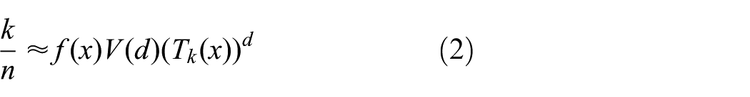
In practice, it may be more convenient to fix the number of neighbors $k$ rather than the radius of the sphere $R$ . Then equation (5) becomes

d_{k} (x) = {(\frac{1}{k - 1} \sum_{j = 1}^{k - 1} \log \frac{T_{k} (x)}{T_{j} (x)})}^{- 1}

(6)

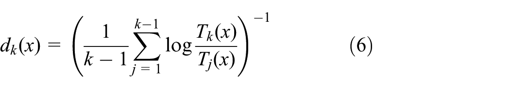
The intrinsic dimensionality $d$ is obtained by setting the range of the neighborhood $k = k_{1}, \dots, k_{2}$

d_{k} = \frac{1}{n} \sum_{i = 1}^{n} d_{k} (x), d = \frac{1}{k_{2} - k_{1} + 1} \sum_{k = k_{1}}^{k_{2}} d_{k}

(7)

Let $G = (V, E)$ be an undirected graph with vertex set $V = {v_{1}, v_{2}, \dots, v_{n}}$ . Where each vertex $v_{i}$ in this graph represents a data point $x_{i}$ and the number of $V$ is $n$ . The respective edge weights $E$ for vertices $(v_{i}, v_{j})$ are determined by the non-negative weight $w_{ij} \geq 0$ , where w_ij = 0 means that there is no connection between vertices $(v_{i}, v_{j})$ . Thus, the distance matrix of vertices $(v_{i}, v_{j})$ is solved by $A_{ij}^{2} = | | x_{i} - x_{j} | |^{2}$ , and the corresponding affinity matrix $w_{ij}$ can be defined as

w_{ij} = {\begin{matrix} \exp (- A_{ij}^{2} / t) & x_{j} \in T_{k} (x_{i}) \\ 0 & otherwise \end{matrix}

(8)

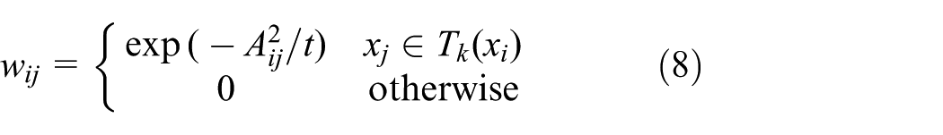
where the parameter $t$ is the thermonuclear width. In this article, the k-nearest neighbor graph was chosen to construct the similarity graphs for dimensionality reduction, and the neighborhood number was $k_{2}$ . The mutual k-nearest neighbor graph was chosen to spectral clustering, and the neighborhood number was $k_{3}$ .

Assume the constructed graph G is connected. Compute eigenvalues and eigenvectors for the generalized eigenvector problem

Ly = λ Dy

(9)

where $D$ is a diagonal matrix, and its entries are column (or row, since $W$ is symmetric) sums of $W$ , $D_{ii} = \sum_{j}^{n} w_{ji}$ . $L = D - W$ is the Laplacian matrix. Laplacian is a symmetric, positive semi-definite matrix which can be thought of as an operator on functions defined on vertices of $G$ .

Let $y_{0}, y_{1}, \dots, y_{n - 1}$ be the solutions of equation (9), order according to their eigenvalues with $y_{0}$ having the smallest eigenvalue (in fact 0). The life-cycle data $Θ^{P} = {x_{1}^{(P)}, x_{2}^{(P)}, \dots, x_{n}^{(P)}}$ under the embedding into the lower dimensional space $Θ^{d}$ is given by ${y_{1} (i), \dots, y_{d} (i)}$ .

Phase 2: adaptive spectral clustering

Adaptive spectral clustering and LE manifold learning are both based on LE algorithm, the difference between them is calculated by the generalized eigenvector problem. LE manifold learning finds a lower dimensional embedding by a pre-defined value, but adaptive spectral clustering determines the degradation state number by the first maximal eigengap. For all clustering algorithms, how to automatically determine the number of clusters is a general problem. Kong et al.⁴⁰ designed the first maximal eigengap for determining the number of clusters. According to the spectral graph theory, in the ideal case of r completely disconnected clusters, the normalized Laplacian matrix contains the eigenvalue as 1 with multiplicity $r$ and then, there is a strict gap to the $(r + 1) th$ eigenvalue that $λ_{d + 1} << 1$ . Thus, the eigengap $g_{i} = λ_{i} - λ_{i + 1}$ can be designed to automatically determine the number of clusters. The practical cases can be considered as the perturbation form of the ideal cases. In this condition, the Laplacian matrix L is not diagonal block. There are r number of eigenvalues are large, such that $λ_{1}, λ_{2}, \dots, λ_{r}$ , but the value of $λ_{r} + 1$ is relatively small. The eigengap $g_{r} = λ_{r} - λ_{r + 1}$ is relatively large. Therefore, the clustering number is determined by the first maximal eigengap sequence

r = \underset{i}{arg min} {g_{i} - g_{j} |_{j < i} > 0 & p g_{i} - g_{i + 1} > 0}

(10)

Note that the input data of adaptive spectral clustering are the low-dimensional embedding $Θ^{d}$ . Let $U \in Θ^{n \times r}$ be the matrix including the first $r$ eigenvectors $u_{1}, u_{2}, \dots, u_{r}$ . Normalized the matrix $U$ , the normalization matrix $U'$ is obtained by

u'_{ij} = \frac{u_{ij}}{{(\sum_{r} u_{ir}^{2})}^{1 / 2}}, i = 1, 2, \dots, n, j = 1, 2, \dots, r

(11)

Therefore, the k-means clustering algorithm is employed to cluster $n$ samples of $U'$ into $r$ clusters $C_{1}, C_{2}, \dots, C_{r}$ .

Fault diagnosis and prognosis

Fault diagnostics and prognostics have received increased attention due their potential to provide early warning of system failures, forecast maintenance as needed, and reduce life-cycle costs. Support vector machine (SVM)^41,42 has been proven to have an excellent generalization capability and has been successfully applied in machinery fault diagnosis. In this article, SVM was chosen to develop fault diagnosis, and Cox proportional hazards model (PHM) was to develop fault prognosis.

Figure 3 shows the flowchart of fault diagnosis and prognosis method. The steps of fault diagnosis and prognosis are summarized as follows:

Step 1. Data acquisition: the monitoring data are collected by sensors installed on the equipment. The historical data are as the training data, and the real-time data are as the testing data.

Step 2. Feature extraction and selection: the monitoring data may be redundant, so that the appropriate degradation indicators are selected in this stage.

Step 3. Data fusion: to improve the effectiveness of fault diagnosis and prognosis, the degradation indicators are processed by LE algorithms. The fusion data are as the input of degradation states segmentation and fault diagnosis, and the first dimensional fusion data as the prognostic parameter.

Step 4. Degradation states segmentation: adaptive spectral clustering is employed to segment the unlabeled monitoring data.

Step 5. Fault diagnosis: SVM is employed to develop fault diagnosis; the corresponding algorithm is described in section “Fault diagnosis based on SVM.”

Step 6. Fault prognosis: Cox PHM is employed to develop fault prognosis; the corresponding algorithm is described in section “Fault prognosis based on Cox PHM.”

Figure 3.

The flowchart of fault diagnosis and prognosis.

Fault diagnosis based on SVM

For linearly separable part, there is an optimal hyperplane $wy + b = 0$ that minimizes $| | w | |^{2}$ . Consider a problem of binary classification where training data are given as $(y_{i}, z_{i}), y \in R^{d}, z_{i} \in {+ 1, - 1}, i = 1, 2, \dots, n$ . The problem of finding a separating hyperplane can be transformed into a quadratic programming problem by Lagrange optimization method

{\begin{matrix} \max w (α) = \sum_{i = 1}^{n} α_{i} - \frac{1}{2} \sum_{i, j = 1}^{n} α_{i} α_{j} z_{i} z_{j} (y_{i}, y_{j}) \\ s . t . \sum_{i = 1}^{n} z_{i} α_{i} \\ α_{i} \geq 0, i = 1, 2, \dots, n \end{matrix}

(12)

where $n$ , $d$ , $z_{i}$ , $α_{i}$ denote sample number, sample dimension, sample classification, Lagrange’s multiplier, respectively. +1 and −1 are the classification labels.

The optimal classification function is

f (y) = sign {(w \cdot y) + b^{*}} = sign {\sum_{i = 1}^{n} α_{i} z_{i} (y_{i} \cdot y) + b^{*}}

(13)

where $α_{i}^{*}$ and $b^{*}$ denote the optimal Lagrange coefficient and classification threshold, respectively. The positive and negative of the classification function are the classification labels.

For linear non-separable part, the main idea is to map the original d-dimensional space into a d′-dimensional space $(d' > d)$ , where the points can possibly be linearly separated. The only operation required in the transformed space is the inner product $ϕ (y_{i})^{T} ϕ (y_{j})$ , which is defined with the kernel function $(K)$ between $y_{i}$ and $y_{j}$ . The common kernel functions are linear kernel function (Linear), polynomial kernel function (Polynomial), the radial basis function (RBF), and a hyperbolic tangent sigmoid kernel function.

The objective function is

w (α) = \sum_{i = 1}^{n} α_{i} - \frac{1}{2} \sum_{i, j = 1}^{n} α_{i} α_{j} z_{i} z_{j} K (y_{i}, y_{j})

(14)

The optimal classification function is

f (y) = sign {\sum_{i = 1}^{n} α_{i} z_{i} K (y_{i} \cdot y) + b^{*}}

(15)

Fault prognosis based on Cox PHM

Let $Z_{i} = {Z_{i 1}, Z_{i 2}, \dots, Z_{ip}}$ be the realized values of the covariates for subject $i$ . The hazard function for the Cox PHM has the form

\begin{array}{l} h (t, Z_{i}) = h_{0} (t) \exp (β_{1} Z_{i 1} + β_{2} Z_{i 2} + \dots + β_{p} Z_{i p}) \\ = h_{0} (t) \exp (β Z_{i}) \end{array}

(16)

where $h_{0} (t)$ , $β$ , and $Z_{i}$ are the baseline hazard function, regression coefficient, and covariate vector, respectively.

The cumulative hazard rate is

H (t, Z_{i}) = \int_{0}^{t} h (t, Z_{i}) dt

(17)

The reliability function is

R (t, Z_{i}) = \exp (- H (t, Z_{i}))

(18)

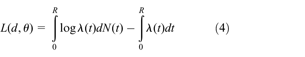
Treating the subjects’ events as if they are statistically independent, the joint probability density of log-likelihood function is

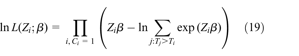
\ln L (Z_{i}; β) = \underset{i, C_{i} = 1}{Π} (Z_{i} β - \ln \sum_{j : T_{j} > T_{i}} \exp (Z_{i} β))

(19)

where $T_{i}$ denotes the observed time (either censoring time or event time) for subject $i$ .

$C_{i}$ is the indicator that the time corresponds to an event (i.e. if C_i = 1, the event occurred and if C_i = 0, the time is a censoring time). The estimate of regression coefficient $β$ can be obtained by maximum likelihood method.

The overall service lifetime can be obtained by

R (t, Z_{i}) = \exp (- H (t, Z_{i})) > RUL con

(20)

where $RUL con$ is the reliability threshold.

The remaining service life can be obtained by

RU L_{estimated} = TOF - T_{current}

(21)

where $TOF$ and $T_{current}$ are the overall service lifetime and current time, respectively.

To evaluate the prognostic performance, the mean absolute percent error (MAPE) is given as

MAPE = mean (\frac{| RU L_{actual} - RU L_{estimated} |}{RU L_{actual}})

(22)

where $RU L_{actual}$ is the actual remaining service life.

Experimental validation

To validate the effectiveness of the proposed method, the run-to-failure tests on turbofan engines were performed. The experimental data were downloaded from the Prognostics Data Repository (http://ti.arc.nasa.gov/project/prognostic-data-repository).⁴³ The data sets consisted of multiple multivariate time series, reflecting the natural degradation of turbofan engines. The dataset 1, namely, train_FD001, test_FD001, and RUL_FD001, was considered in this article. In the training set, the fault grows in magnitude until system failure. In the test set, the time series ends some time prior to system failure. RUL_FD001 provides a vector of true remaining useful life (RUL) values for the test data. The dataset contained 24 element vectors consisted of 3 operational settings and 21 sensor measurements.⁴⁴ The total lifetime for each engine in the training set is shown in Figure 4. It can be seen from Figure 4 that the lifetime varies from 128 to 362 cycles (mean = 206.3 cycles, standard deviation = 46.34 cycles).

Figure 4.

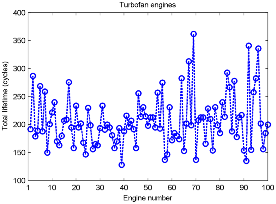
Actual lifetime of each engine in the training set.

Degradation state segmentation

To improve the effectiveness of fault diagnosis and prognosis and reflect the natural degradation of turbofan engines, the respective features are selected. For fault diagnosis, the 24 features are as the degradation indicators. By automatic segmentation in section “Automatic segmentation algorithm,” the dimension of the life-cycle data (24-dimension) was reduced into 6-dimension. 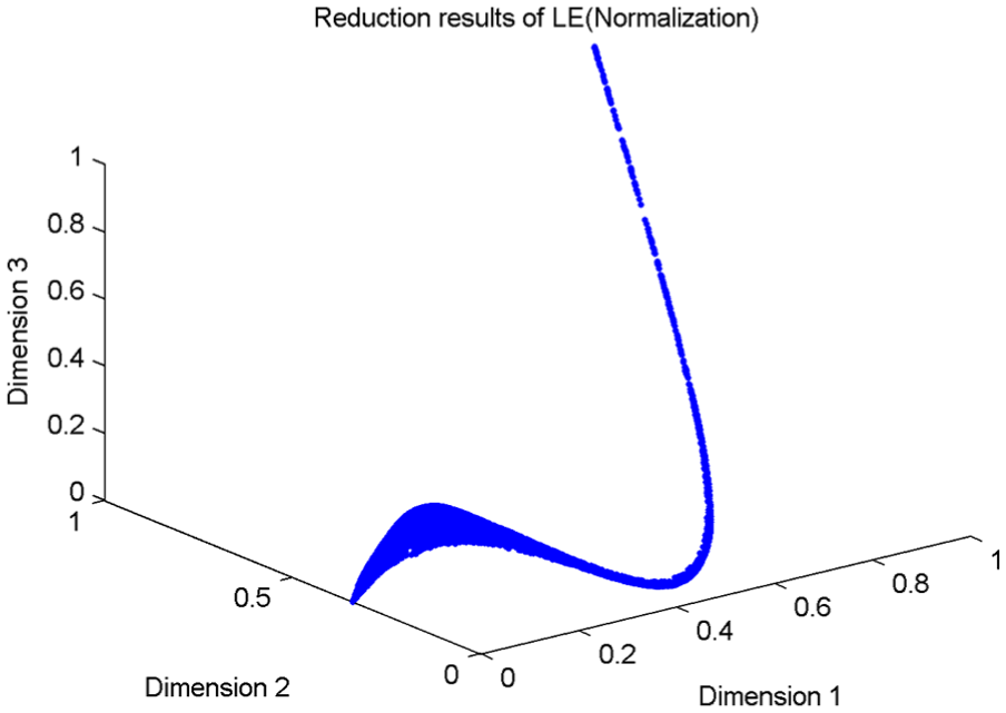Where, the neighborhood number in Phase 1 was in the range of 6–12, and the neighborhood number $k_{2}$ and parameter $t$ were 12 and 1, respectively. The first three-dimension of the reduction results is selected for visualization, which is shown in Figure 5. Note that here the output of LE manifold learning is four-dimensional data.

Figure 5.

Visualization of the reduction results by LE manifold learning.

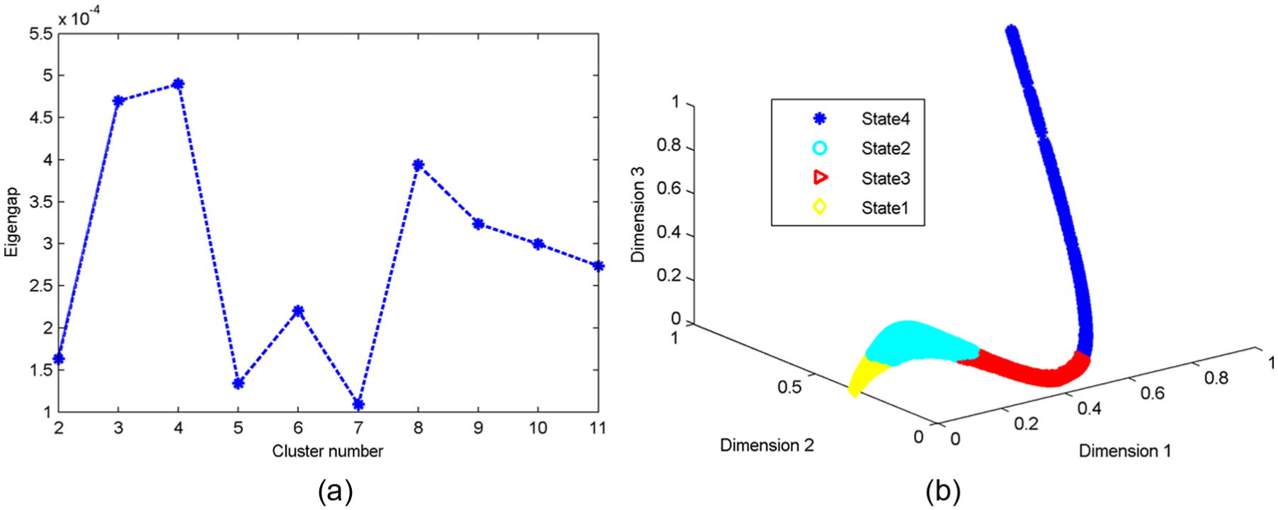
By Phase 2 in section “Automatic segmentation algorithm” with the output of Phase 1, the state number and class label were obtained. Where, the neighborhood number $k_{3}$ and parameter $t$ in Phase 2 were 15 and 1, respectively. Figure 6(a) shows the estimation results of degradation states number, and the corresponding state is shown in Figure 6(b). From Figure 6, it can be seen that the turbofan engine will go through $r = 4$ degradation states from time zero to failure. The degradation state $1 \to r$ indicates the system performance is a gradual deterioration process. Where state 1 denotes the perfect performance of the system, state $r$ denotes the worst performance of the system. The performance of the system is gradual degradation in this order. The output of the automatic segmentation method can be considered as the available information for developing fault diagnosis.

Figure 6.

Results of automatic segmentation: (a) estimation of degradation states number and (b) results of adaptive spectral clustering.

Fault diagnosis

For fault diagnosis, the engines No. 1–No. 60 are taken as the train samples and the engines No. 81–No. 100 are taken as the test samples. Note that here the samples are random distribution, and the optimal parameters of SVM are found by grid search algorithm, and the cluster labels are considered as the true labels of turbofan engine. The diagnosis results by SVM are compared with the true labels, which are shown in Figure 7. The diagnosis accuracy is 99.55%. The respective corresponding degradation states of No. 94 engine and No. 82 engine over the operational time are shown in Figure 8. It can be seen that two engines start with different initial operational states owing to different degrees of initial wear and manufacturing variation which is unknown to the user. This wear or variation is considered normal, that is, it is not considered a fault condition. No. 94 engine goes through four degradation states, while No. 82 engine only three degradation states. The results indicate that No. 82 engine is operated at degradation state 2, and No. 94 engine has the higher reliability in the initial operational state than No. 82 engine. The reason is that products exist the difference in material and manufacturing process.

Figure 7.

SVM diagnosis results.

Figure 8.

Degradation states of No. 94 engine and No. 82 engine.

Fault prognosis

For fault prognosis, train_FD001 are taken as the training samples, test_FD001 are taken as the testing samples. The literature^45,46 suggested the features ${7, 8, 12, 16, 17, 20}$ led to the best prognostic performance. In this article, we also chose the features ${7, 8, 12, 16, 17, 20}$ as the degradation indicators for fault prognosis. By Cox PHM in section “Fault prognosis based on Cox PHM,” the Cox PHM RUL estimation result of RULcon = 0.9 and RULcon = 0.95 are shown in Figures 9 and 10, respectively. Where the estimated value of β = 37.6364 and the covariate vector are the first dimensional fusion data. It can be seen from Figures 9 and 10, the $MAPE$ values of RULcon = 0.9 and RULcon = 0.95 are 50.2934 and 56.809, respectively. To better evaluate the prognostic performance, Cox PHM RUL estimation method was compared with Weibull estimation. Figure 11 shows the Weibull estimated results. Where the estimated values of $α$ and $η$ are 4.4087 and 225.0258, respectively, and the $MAPE$ value of Weibull estimation is 98.5072. It is concluded that Cox PHM is more suitable to predict the remaining service life than Weibull estimation and has achieved a good performance. Where the Weibull failure rate is

λ (t) = \frac{α}{η} {(\frac{t}{η})}^{α - 1}

(23)

where $α$ and $η$ are shape parameter and scale parameter, respectively.

Figure 9.

Cox PHM estimated results of RULcon = 0.9: (a) Cox PHM RUL estimates and (b) Cox PHM RUL estimation error: MAPE = 50.2934.

Figure 10.

Cox PHM estimated results of RULcon = 0.95: (a) Cox PHM RUL estimates and (b) Cox PHM RUL estimation error: MAPE = 50.809.

Figure 11.

Weibull estimated results: (a) Weibull RUL estimates and (b) Weibull RUL estimation error: MAPE = 98.5072.

The mean remaining service life of Weibull estimation is estimated by

RU L_{estimated} = \frac{1}{S (t)} \int_{t}^{+ \infty} S (t) dt

(24)

where $t$ is the current time, and $S (\cdot)$ is the survival function.

From the above results, the automatic segmentation has been proven to be a high-efficiency and feasibility method, which can automatically find the low-dimensional embedding and determine the structure of the degradation model. Thus, the data uncertainty can be eliminated, which is of great significance for fault diagnosis and prognosis.

Additionally, the main challenge in the automatic segmentation method is the available life-cycle data. Finding a reasonable model which requires large amount of data is usually not available in real world. The overall accuracy of fault diagnosis/prognosis will be seriously affected by the insufficient data. Moreover, selection of the monotonous features representing the degradation progression is a prerequisite for effective fault prognostics. However, the performance of the automatic segmentation method itself is sufficiently accurate.

Conclusion

In this article, an automatic segmentation was performed, which was validated through three artificial data sets and the run-to-failure experiments of turbofan engine. The results suggest that the automatic segmentation method has effectively overcome the curse of dimensionality and eliminated the degradation process uncertainty. It is a high-efficiency and feasibility method for model selection of high-dimensional data.

The proposed approach has three main benefits. First, only the performance monitoring data are required but not the prior knowledge about the equipment or the operating conditions. Second, the method can be employed in single or multiple operating conditions. Third, the method not only can deal with low-dimensional data (directly Phase 2) and high-dimensional data but also the non-convex and convex data. Therefore, the proposed method can be seamlessly applied to any mechanical equipment, and the output of the automatic segmentation method can be considered as the available information for developing fault diagnosis/prognosis.

Footnotes

Academic Editor: Yangmin Li

Declaration of conflicting interests

The author(s) declared no potential conflicts of interest with respect to the research, authorship, and/or publication of this article.

Funding

The author(s) received no financial support for the research, authorship, and/or publication of this article.

References

Litt

. An optimal orthogonal decomposition method for Kalman filter-based turbofan engine thrust estimation. J Eng Gas Turb Power 2008; 130: 011601.

Tayarani-Bathaie

Vanini

Khorasani

. Dynamic neural network-based fault diagnosis of gas turbine engines. Neurocomputing 2014; 125: 153–165.

Ramasso

Saxena

. Review and analysis of algorithmic approaches developed for prognostics on CMAPSS dataset. In: Proceedings of the annual conference of the prognostics and health management society, Fort Worth, TX, USA, September 2014.

Donat

Choi

et al . Data visualization, data reduction and classifier fusion for intelligent fault diagnosis in gas turbine engines. J Eng Gas Turb Power 2008; 130: 041602.

Ramasso

Gouriveau

. Prognostics in switching systems: evidential Markovian classification of real-time neuro-fuzzy predictions. In: Proceedings of the prognostics and health management conference, 2010 (PHM’10), Macao, China, 12–14 January 2010, pp.1–10. New York: IEEE.

Feng

Xiao

Liu

et al . A kernel principal component analysis–based degradation model and remaining useful life estimation for the turbofan engine. Adv Mech Eng. Epub ahead of print 20 May 2016. DOI: 10.1177/1687814016650169.

Dewallef

Borguet

. A methodology to improve the robustness of gas turbine engine performance monitoring against sensor faults. J Eng Gas Turb Power 2013; 135: 051601.

Dewallef

Romessis

Léonard

et al . Combining classification techniques with Kalman filters for aircraft engine diagnostics. J Eng Gas Turb Power 2006; 128: 281–287.

Chang

Huang

et al . Gas-path health estimation for an aircraft engine based on a sliding mode observer. Energies 2016; 9: 598.

10.

Zheng

Huang

et al . Life cycle performance estimation and in-flight health monitoring for gas turbine engine. J Dyn Syst Meas Control 2016; 138: 091009.

11.

Dreiseitl

Ohno-Machado

. Logistic regression and artificial neural network classification models: a methodology review. J Biomed Inform 2002; 35: 352–359.

12.

Romessis

Mathioudakis

. Bayesian network approach for gas path fault diagnosis. J Eng Gas Turb Power 2006; 128: 64–72.

13.

Ogaji

Singh

. Advanced engine diagnostics using artificial neural networks. Appl Soft Comput 2003; 3: 259–271.

14.

Ramasso

. Contribution of belief functions to hidden Markov models with an application to fault diagnosis. In: Proceedings of the IEEE international workshop on machine learning for signal processing (MLSP 2009), Grenoble, 1–4 September 2009, pp.1–6. New York: IEEE.

15.

. Hidden semi-Markov models. Artif Intell 2010; 174: 215–243.

16.

Peng

Dong

. A prognosis method using age-dependent hidden semi-Markov model for equipment health prediction. Mech Syst Signal Pr 2011; 25: 237–252.

17.

Kim

Ball

Nwadiogbu

. Fault diagnosis in turbine engines using unsupervised neural networks technique. In: Proceedings of the SPIE defense and security, Orlando, FL, April 2004, pp.150–158. Bellingham, WA: International Society for Optics and Photonics.

18.

Moghaddass

Zuo

. A parameter estimation method for a condition-monitored device under multi-state deterioration. Reliab Eng Syst Safe 2012; 106: 94–103.

19.

Kouropteva

Okun

Pietikäinen

. Incremental locally linear embedding. Pattern Recogn 2005; 38: 1764–1767.

20.

Van der Maaten

LJP

Postma

Van Den

. Dimensionality reduction: a comparative review. Technical report, Maastricht University, Maastricht, May 2007.

21.

Levina

Bickel

. Maximum likelihood estimation of intrinsic dimension. In: Proceedings of the advances in neural information processing systems, Vancouver, BC, Canada, 13–18 December 2004, pp.777–784. New York: Association for Computing Machinery.

22.

Qin

Liu

. A novel approach to update summarization using evolutionary manifold-ranking and spectral clustering. Expert Syst Appl 2012; 39: 2375–2384.

23.

Prastawa

Gilmore

Lin

et al . Automatic segmentation of MR images of the developing newborn brain. Med Image Anal 2005; 9: 457–466.

24.

Creutz

. Induction of the morphology of natural language: unsupervised morpheme segmentation with application to automatic speech recognition. Helsinki University of Technology, 2006, http://lib.tkk.fi/Diss/2006/isbn9512282119/isbn9512282119.pdf

25.

Ramasso

Denoeux

. Making use of partial knowledge about hidden states in HMMs: an approach based on belief functions. IEEE T Fuzzy Syst 2014; 22: 395–405.

26.

Ramasso

Gouriveau

. Remaining useful life estimation by classification of predictions based on a neuro-fuzzy system and theory of belief functions. IEEE T Reliab 2014; 63: 555–566.

27.

Ramasso

Rombaut

Zerhouni

. Joint prediction of continuous and discrete states in time-series based on belief functions. IEEE T Cyb 2013; 43: 37–50.

28.

De Ridder

Duin

. Sammon’s mapping using neural networks: a comparison. Pattern Recogn Lett 1997; 18: 1307–1316.

29.

Cao

Chua

Chong

et al . A comparison of PCA, KPCA and ICA for dimensionality reduction in support vector machine. Neurocomputing 2003; 55: 321–336.

30.

Samko

Marshall

Rosin

. Selection of the optimal parameter value for the Isomap algorithm. Pattern Recogn Lett 2006; 27: 968–979.

31.

Roweis

Saul

. Nonlinear dimensionality reduction by locally linear embedding. Science 2000; 290: 2323–2326.

32.

Belkin

Niyogi

. Laplacian eigenmaps for dimensionality reduction and data representation. Neural Comput 2003; 15: 1373–1396.

33.

Weinberger

Saul

. An introduction to nonlinear dimensionality reduction by maximum variance unfolding. In: Proceedings of the 21st national conference on artificial intelligence (AAAI’06), Boston, MA, 16–20 July 2006, vol. 6, pp.1683–1686. New York: Association for Computing Machinery.

34.

Maaten

LVD

Hinton

. Visualizing data using t-SNE. J Mach Learn Res 2008; 9: 2579–2605.

35.

Van Der Maaten

Postma

Van den Herik

. Dimensionality reduction: a comparative. J Mach Learn Res 2009; 10: 66–71.

36.

Van der Maaten

. Learning a parametric embedding by preserving local structure. RBM 2009; 500: 26.

37.

Van Der Maaten

. Accelerating t-SNE using tree-based algorithms. J Mach Learn Res 2014; 15: 3221–3245.

38.

Camastra

. Data dimensionality estimation methods: a survey. Pattern Recogn 2003; 36: 2945–2954.

39.

Carter

Raich

Hero

III . On local intrinsic dimension estimation and its applications. IEEE T Signal Proces 2010; 58: 650–663.

40.

Kong

Sun

et al . Automatic spectral clustering and its application. In: Proceedings of the 2010 international conference on intelligent computation technology and automation (ICICTA), Changsha, China, 11–12 May 2010, vol. 1, pp.841–845. New York: IEEE.

41.

Hsu

Chang

Lin

. A practical guide to support vector classification, 2003, http://www.csie.ntu.edu.tw/∼cjlin/papers/guide/guide.pdf

42.

Chang

Lin

. LIBSVM: a library for support vector machines. ACM Trans Intell Syst Tech 2011; 2: 27.

43.

Saxena

Goebel

Simon

et al . Damage propagation modeling for aircraft engine run-to-failure simulation. In: Proceedings of the international conference on prognostics and health management (PHM 2008), Denver, CO, 6–9 October 2008, pp.1–9. New York: IEEE.

44.

Liu

Huang

. Integration of data fusion methodology and degradation modeling process to improve prognostics. IEEE T Autom Sci Eng 2016; 13: 344–354.

45.

Soumik

Jin

Asok

. Data-driven fault detection in aircraft engines with noisy sensor measurements. J Eng Gas Turb Power 2011; 133: 783–789.

46.

Ramasso

. Investigating computational geometry for failure prognostics. PHM Soc 2014; 5: 1–18.

Automatic segmentation and prognostic method of a turbofan engine using manifold learning and spectral clustering algorithms

Abstract

Keywords

Introduction

The procedure of automatic segmentation method

Automatic segmentation algorithm

Phase 1: manifold learning dimensionality reduction

Phase 2: adaptive spectral clustering

Fault diagnosis and prognosis

Fault diagnosis based on SVM

Fault prognosis based on Cox PHM

Experimental validation

Degradation state segmentation

Fault diagnosis

Fault prognosis

Conclusion

Footnotes

Declaration of conflicting interests

Funding

References