Stabilization of pilot valve system using linear flow resistance

Abstract

In a pilot valve system, the pressure in the control chamber of the main valve is straightforwardly affected by pressure oscillation in the downstream pipeline or the pilot tube. To solve this problem, an orifice is generally installed in the pilot tube to restrain the oscillation. However, the orifice is a nonlinear flow resistance; the amplitude of the oscillation alters the gain curve of the control pressure response. In this study, a linear flow resistance such as a porous material is employed to stabilize the pilot valve system. A test pilot valve was manufactured, and a pilot valve system was developed in the laboratory of the authors of this article. A mathematical model of the pilot valve system using linear and nonlinear flow resistances was simulated in MATLAB. The linearity of the P–Q characteristics of the linear flow resistance was confirmed, and a series of frequency response experiments were performed to examine the dynamic characteristics of the pilot valve system with various flow resistances. The experimental results were in accord with the simulation results. This implied that when porous materials were used in the pilot valve system, the gain of the pressure response did not vary regardless of the varying pressure vibration amplitude. Therefore, porous materials are suitable to be used in the pilot valve system instead of an orifice to enhance its stability.

Keywords

Porous material orifice pilot valve linear flow resistance flow rate characteristics dynamic experiment

Introduction

In a medium-pressure gas pipeline, a pilot valve system is usually used in a gas governor unit to control the downstream pressure as it can reduce the offset of the secondary pressure.¹ The flow rate of the gas pipeline is regulated by the main valve. The pressure in the diaphragm chamber of the main valve is adjusted by the flow rate through the pilot tube (see Figure 1), and the flow rate is controlled by the pressure in the diaphragm chamber of the pilot valve. Numerous researchers focus on the analysis of flow field in various pilot valves by computational fluid dynamics (CFD) methods. Lv et al.² presented the flow field characteristics in a flapper-nozzle pilot valve when the flapper is moving, which reflects the actual operational conditions. Yuan and Guo³ developed complete models of the pilot relief valve using deformation theory of thin plates. Qian et al.^4,5 analyzed the dynamic flow characteristics and cavitation characteristics in a pilot-control globe valve. Their research studies can support design initiatives for further optimization and engineering applications of the pilot valve system. However, these studies are limited to the theoretical investigation of the pilot valve; the actual problems of the pilot valve system in gas pipelines are not adequately described in the literature.

Figure 1.

Pilot-type governor unit.

Recently, a gas company observed the occurrence of resonant vibrations of the gas column⁶ in the pilot tube. In addition, oscillations of secondary pressure are generally observed in the downstream pipeline. A number of factors cause these problems, such as dead bands⁷ and choking flow, at the restrictions⁸ and the self-excited vibration of the moving component in the valve.⁹ The control pressure in the main valve is straightforwardly affected by all these vibrations, and these vibrations cause pressure response oscillations, resulting in secondary pressure instability. Pressure feedback can amplify the vibrations and can render the gas equipment unusable.¹⁰

Generally, for preventing pressure oscillation caused by self-induced vibration of the pilot valve, the resistance of the pilot valve can be increased by increasing the friction in the valve stem and mass of the diaphragm and reducing the area of the diaphragm. For reducing the unstable pressure in the diaphragm chamber caused by the pressure oscillation in the pilot tube and downstream pipeline, a reference method that can be adopted is to enlarge the volume of the diaphragm chamber of the pilot valve and main valve. However, all these methods require modifications in the structure of the valve. Meanwhile, restricting the pressure feedback line is an effective method¹¹ to restrain the effect of downstream pressure vibration. Gas governor manufacturers install a flow resistance, such as an orifice, in the pilot tube; such designs can be observed in numerous past pilot valve patents.^12–14 In certain pilot valve systems, the orifice is also a key component to control the action of the valve; a few literatures demonstrate the effect of an orifice in the pilot-control globe valve¹⁵ and pilot-operated pressure relief valve¹⁶ using numerical methods. However, the flow resistance of an orifice is nonlinear; the gain and phase curves of the pressure response in a bode diagram varies with the amplitude of the pressure oscillation.^17–19 This implies that when the amplitude of the vibration varies, the amplitude magnitudes of the pressure response in the diaphragm chamber reduce by varying proportions at similar vibration frequency. Hence, it is a challenge for engineers to judge the stability of the system. As is known, the flow rate is proportional to the pressure difference when the flow state is transformed to a laminar flow in certain microstructures with low Reynolds numbers. This implies that certain microstructures exhibit linear flow characteristics; they are defined as linear flow resistances. A few researchers observed that porous materials exhibit linear flow rate characteristics when viscous effects govern the flow, which is referred to the Darcy regime.^20–25 The pressure exceeds Darcy regime to a substantial degree; it is not feasible to attain this high with the pressure oscillation in the gas pipeline. Therefore, high-pressure conditions were not considered in this research study.

In our previous research study,²⁶ the dynamic characteristics of a pneumatic resistance-capacitance (RC) circuit with porous materials were investigated. In this study, a porous material is employed to stabilize the pilot valve system considering its linear flow resistance characteristics. The linear characteristics of these porous materials can be attributed to the fact that the flow state in their micro holes shifts to laminar. The P–Q characteristics curves of the porous materials were measured by performing a static flow rate experiment. Generally, the volume flow rate in a gas governor unit is higher than 2000 m³/h; however, it is challenging to perform an experiment with such a large flow rate in the laboratory of the authors of this article. Therefore, a test pilot valve was manufactured, and a pilot valve system was developed to evaluate the influence of the downstream pressure oscillation on the control pressure response. A mathematical model of this pilot valve system using linear flow resistance and nonlinear flow resistance was simulated in MATLAB. Then, a series of frequency response experiments were carried out to investigate the dynamic characteristics of the pilot valve testing system with various flow resistances. The experimental results were compared with the simulation results. The effect of the linear flow resistance on the dynamic characteristics of the pilot valve system was examined in this research study. The conclusions imply that porous materials are suitable for use, instead of an orifice, in a pilot valve system to enhance its stability.

Pilot valve testing system

Pilot valve system is a representative category of gas governor units. Figure 1 illustrates a common pilot valve system. A main valve (called the axial flow valve) is installed in the main gas pipeline, and a pilot valve is installed in the pilot line. When the downstream pressure P₂ decreases, the change is detected by the pilot tube, which is restricted by restriction 2. Then, the pressure P_d acting on the diaphragm of the pilot valve also drops, and the valve opens. The gas flows into the pilot line from the diaphragm chamber of the main valve, and the main valve opens because of the drop in the control pressure P_c. The flow rate Q₂ and downstream pressure P₂ increase and feedback to the pilot valve. Eventually, the system returns to a new equilibrium state. It can be observed that the downstream pressure oscillation affects the pressure P_d in the pilot valve instantaneously and affects the control pressure P_c in the main valve indirectly.

The flow rate is substantially large in the main pipe, and it is not feasible to generate such a flow rate in our laboratory. Therefore, in the pilot valve testing system (Figure 2), the diaphragm chamber of the main valve was replaced with an isothermal chamber (ITC),²⁷ and the main pipe was removed. The pressure in the ITC continued to be referred to as control pressure P_c. A sine-wave pressure P_i, instead of the downstream oscillation, was provided by a pressure generator. The upstream pressure P₁ was maintained constant by the pressure regulator. To evaluate the characteristics of the pilot valve testing system, the pressure responses of P_c and P_d relative to P_i were measured under various test restrictions. In this test system, it is convenient to observe the pressure response results under similar experimental conditions. The pressure P_i can be maintained as a sine wave because there is no feedback flow to affect it.

Figure 2.

Pilot valve testing system.

Linear and nonlinear flow resistances

Pressure–flow (P–Q) characteristics curve is a critical characterization of flow resistance. A static flow rate experiment was performed to ascertain the P–Q characteristics of the restrictions. Figure 3 illustrates the pneumatic devices of the static experiment. In this experiment, air was used instead of any specific gas because of the safety that it affords and thermodynamic similarity. The flow rate Q was adjusted by the control valve and recorded by the quick flow sensor (QFS). The differential pressure was obtained from pressure sensors P₁ and P₂.

Figure 3.

Static experimental setup.

A porous material was used as a test restriction in this experiment. The dimensions and shape of the material are illustrated in Figure 4. The porous material is a sintered metal element with a filter precision of 2 μm. The arrows at the right panel in Figure 4 illustrate the flow route through the material and its package case, and it indicates that the effective area of the porous material is the inner wall of the hollow cylinder. Porous materials are linear flow resistances, that is, its flow rate is proportional to the pressure. Therefore, the flow equation is a linear equation, and the linear fitting equation can be obtained through the experimental data on P–Q characteristics.

Figure 4.

Porous material specimen.

The other test restriction used is an orifice, which has an inner diameter of 2.8 mm. The nonlinear flow rate equation²⁸ (equation (1)) of the orifice is

\begin{matrix} When \frac{P_{D}}{P_{U}} \leq 0.5283, G (S_{e}, P_{U}, P_{D}) \\ = S_{e} P_{U} \sqrt{\frac{κ}{R θ_{1}} {(\frac{2}{κ + 1})}^{\frac{κ + 1}{κ - 1}}} \end{matrix}

(1a)

\begin{matrix} When \frac{P_{D}}{P_{U}} > 0.5283, G (S_{e}, P_{U}, P_{D}) \\ = S_{e} P_{U} \sqrt{\frac{2 κ}{κ - 1} \cdot \frac{1}{R θ_{1}} [{(\frac{P_{D}}{P_{U}})}^{\frac{2}{κ}} - {(\frac{P_{D}}{P_{U}})}^{\frac{κ + 1}{κ}}]} \end{matrix}

(1b)

S_{e} = C_{D} \frac{π d^{2}}{4}

(2)

where R is the ideal gas constant, P_U is the upstream pressure, P_D is the downstream pressure, θ₁ is the flow temperature, κ is the specific heat ratio, S_e is the effective area, d is the diameter of the orifice, and C_D is the discharge coefficient.

Figure 5 illustrates the P–Q characteristic curves for the various flow resistances. The diamond- and triangle-shaped points represent the experimental data of the porous material and orifice, respectively. The results demonstrate that the experimental data points of the porous material are distributed along a straight line, whereas the data points of the orifice are distributed along a curve. From the experimental data, the discharge coefficient C_D for this orifice was calculated to be 0.93, with the upstream pressure set to 90 kPa. For an upstream pressure of 150 kPa, the P–Q characteristic curve for the orifice is represented by the dashed curve in Figure 5. The fitted equation of the P–Q characteristics (straight line) for the porous material was determined to be

Q_{p} = 11.6 * Δ P

(3)

Here, Q_p is the quantity of flow, and ΔP is the differential pressure. The pressure and flow rate are measured in units of kPa and L/min, respectively.

Figure 5.

P–Q characteristic curves.

Simulation

The test pilot valve was manufactured by Tokyo Gas Co., Ltd (Figure 6). An orifice (restriction 1) located upstream is embedded in the inlet of the valve. The diaphragm chamber is isolated from the downstream volume to avoid the effect of the downstream pressure. The control chamber is connected to an ITC to enlarge the volume and eliminate the change in temperature. The mathematical model of this system constitutes three components: the pneumatic RC circuit with the restriction and diaphragm chamber, pilot valve model, and control chamber isothermal model.

Figure 6.

Model of pilot valve testing system.

Mathematical model of pneumatic RC circuit

The pressure vibration was simulated by a sine-wave pressure source. The mass flow rate G_d through the orifice and porous materials were obtained from equations (1) and (3). The volume in the diaphragm chamber¹⁷ was assumed to be constant, and the ideal gas equation applied was the following

P_{d} V_{d} = mR θ

(4)

Differentiating equation (4) with respect to time yields the following

\frac{V_{d} d P_{d}}{dt} = R θ \frac{dm}{dt} + mR \frac{d θ}{dt}

(5)

where P_d is the pressure in the diaphragm chamber, V_d is the volume, m is the mass of the air in the chamber, and θ is the average temperature. Note that dm/dt is the mass flow rate G_d.

Considering the enthalpy in the diaphragm chamber and the energy variation along the wall, the energy equation was obtained from the first law of thermodynamics

q = P_{d} \frac{G_{d}}{ρ} - C_{v} ρ V_{d} \frac{d θ}{dt}

(6)

where ρ is the average density of air in the diaphragm chamber, C_v is the constant volume specific heat capacity, C_v = 718 J/(kg K), and q is the heat transfer along the wall. Using Newton’s law of cooling, q is defined as

q = h S_{h} (θ - θ_{a})

(7)

where θ_a is the temperature of the atmosphere, h is the thermal conductivity, and S_h is the heat transfer area of the diaphragm chamber. Equation (7) is substituted in equation (6) to obtain

\frac{d θ}{dt} = \frac{R θ}{C_{v} P_{d} V_{d}} {R θ G_{d} - h S_{h} (θ - θ_{a})}

(8)

By substituting equation (8) in equation (5) and using the equation R = C_p−C_v, where C_p is the constant pressure specific heat capacity (C_p = 1005 J/(kg K)), the following equation is obtained

\frac{{dP}_{d}}{dt} = \frac{R}{C_{v} V_{d}} {C_{p} θ G_{d} - h S_{h} (θ - θ_{a})}

(9)

Mathematical model of test pilot valve

The mass flow rate G_N through the nozzle flapper of the valve can also be obtained using equation (1), that is, G_N = G (S_ex, P_c, P_o). Here, S_ex is the effective area of the nozzle flapper and is defined as

S_{ex} = C_{D} π d_{N} x

(10)

where x is the displacement between the nozzle and flapper, and d_N is the diameter of the nozzle. x depends on the dynamic equation of the valve, and thus

m_{v} \frac{d^{2} x}{d t^{2}} + c \frac{dx}{dt} + (k_{1} + k_{2}) x = (P_{d} - P_{set}) A_{d}

(11)

where m_v is the total mass of the moving component and includes the mass of the flapper and center plates and one third of the sum of the spring mass, c is the damping in the valve, k₁ is the spring constant of the adjustment spring, k₂ is the spring constant of the counter spring, P_set is the set pressure of the valve, and A_d is the effective area of the diaphragm. The Coulomb friction was neglected in this equation because it was negligible in the test valve.

Mathematical model of ITC

In the ITC, the temperature is constant. Therefore, by removing the temperature term, equation (5) can be written as

\frac{V_{c} d P_{c}}{dt} = R θ_{a} (G_{1} - G_{N})

(12)

where V_c is the sum of the volumes of the ITC, control chamber, and pipe; P_c is the control pressure; G₁ is the flow rate through orifice 2 in the valve; G₁ = G (S_e₂, P₁, P_c); and S_e₂ is the effective area of orifice 2.

Finally, to simplify the calculation, the ITC continues to be used for the downstream volume as it is not a critical part of this simulation. Thus

\frac{V_{o} d P_{o}}{dt} = R θ_{a} (G_{N} - G_{2})

(13)

where V_o is the downstream volume, P_o is the downstream pressure, G₂ is the mass flow rate through the outlet of the valve, G₂ = G (S_e₃, P_o, P_a), and S_e₃ is the effective area of the outlet.

The gains of P_c and P_d are defined as

GAI N_{c} = 20 \log_{10} (\frac{A_{c}}{A_{i}}), GAI N_{d} = 20 \log_{10} (\frac{A_{d}}{A_{i}})

(14)

where A_c, A_d, and A_i are the amplitudes of P_c, P_d, and P_i, respectively. The phase difference Δϕ_c with respect to the input pressure is also considered, that is

Δ ϕ_{c} = ϕ_{c} - ϕ_{i}

(15)

Here, ϕ_c and ϕ_i are the phases of P_c and P_i, respectively.

The simulation was implemented in Simulink, which is integrated with MATLAB. The Runge–Kutta algorithm was adopted to calculate the simulation models. The solver selects the fixed-step solver; the step size of the sample time was set to 0.0001 s; Figure 7 illustrates the simulation block diagram.

Figure 7.

Block diagram of simulation.

Experimental dynamic characteristics

A frequency response experiment was performed to investigate the dynamic response of the pilot valve testing system using the porous materials and orifice.

Experimental apparatus

Figure 8 illustrates the pneumatic circuit used in the frequency response experiment. A pressure generator was designed to provide a sine-wave pressure input. In this pressure generator, the inflow and outflow from a control chamber is regulated by a servo valve using proportional–integral (PI) feedback control. The generated input pressure P_i and the response pressures in the diaphragm chamber (P_d) and ITC (P_c) were recorded by pressure sensors. Figure 9 presents an image of the experimental apparatus. Table 1 lists the specifications of the devices used in the experiment.

Figure 8.

Pneumatic circuit diagram of dynamic experiment.

Figure 9.

Photograph of experimental apparatus.

Table 1.

Specifications of the experimental devices.

Equipment	Range	Type
Pressure P_i	0–500 kPa	FP101-B31-C20A*B (YOKOGAWA)
Pressure P_d	0–200 kPa	FP101-A31-C20A*B (YOKOGAWA)
Pressure P_c	0–1 MPa	AP-13S (KEYENCE)
Flow rate	0–200 L/min	QFS-200 (TOKYO METER)
ITC	180 mL	ITC-0.2 (TOKYO METER)

ITC: isothermal chamber.

The experimental conditions are listed in Table 2. All the pressure values are recorded relative to the pressures in the succeeding component of the apparatus. The data of P_i, P_c, and P_d were recorded while increasing the frequency at similar input amplitude. The test valve started to open at the set pressure of 161 kPa, and the base value of P_i was set to 150 kPa. Therefore, the amplitude was limited to 10 kPa because the valve reached full-open and full-close states when the amplitude exceeded 10 kPa.

Table 2.

Experimental conditions.

Test restriction	Frequency (Hz)	Amplitude (kPa)
Porous	1–25	2, 5, 10
Orifice	1–25	2, 5, 10

Simulation and experimental results

The pressure generator can produce a reasonable sine-wave pressure P_i at low frequencies albeit not at high frequencies, as illustrated in Figure 10 (frequency: 20 Hz). Therefore, the data were processed by carrying out harmonic analysis based on the fast Fourier transform (FFT) technique to confirm the amplitude and phase accuracy. Figure 11 illustrates the shape of the experimental sine-wave pressures P_d and P_c at various frequencies for the porous material. The amplitudes of P_d and P_c decrease as the frequency increases because of the damping of the pneumatic RC circuit and test pilot valve.

Figure 10.

Pressure wave for porous material (f = 20 Hz, A_i = 10 kPa).

Figure 11.

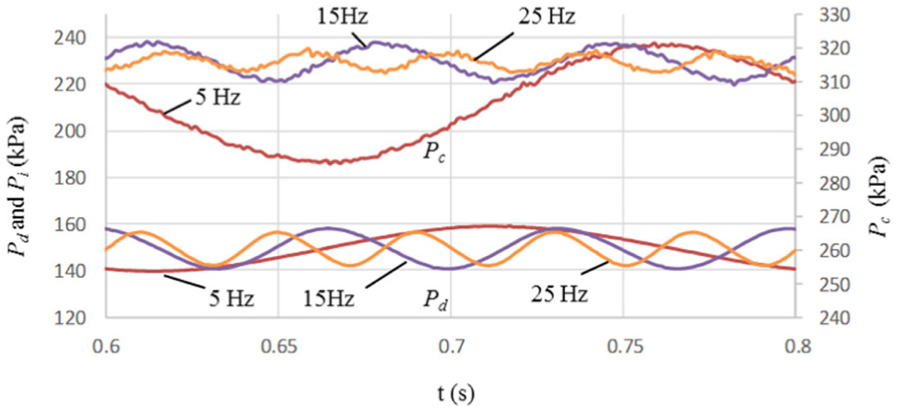
Pressure wave for porous material at various frequencies (A_i = 10 kPa).

Based on the definitions in equations (14) and (15), the variations in the Bode diagram of P_c with the frequency are illustrated in Figure 12. The points represent the measurement data, whereas the various markers denote the various amplitude conditions of the sine-wave input pressure. The colors denote the various restrictions. The red-dashed curve represents the simulation results of the porous material when the amplitudes of the input pressure P_i are 2, 5, and 10 kPa. The simulation results demonstrate that the gain drop curve of P_c as the frequency increases is constant with varying amplitude of the input pressure vibration, when the porous material is used as the test restriction. The experimental data for various amplitudes of the input pressure were in agreement considering that the data points were all located in the proximity of the same simulation curve. However, for the orifice, the gain curves are of three forms at high frequencies for various input amplitudes. The simulation results represented by the three blue solid curves and the distribution of the data points are also in high agreement with these curves. Thus, if the amplitude conditions of the input pressure varies, the pressure gain P_c drops at a different rate when the orifice is used as the test restriction. In addition, the width of the gain variation is approximately 5 dB at 25 Hz at input amplitudes between 2 and 10 kPa. The diagram of phase difference also follows the rules of this variation (Figure 12(b)).

Figure 12.

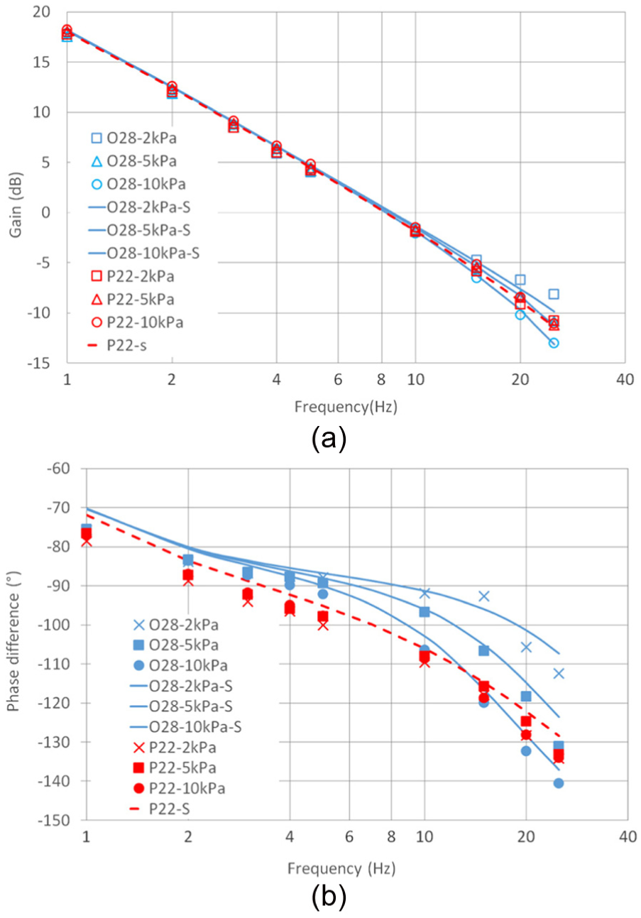
Frequency response of control pressure P_c: (a) gain and (b) phase difference between P_c and P_i.

At low frequencies, the gain and phase difference variations are approximately similar irrespective of the restriction used because by this time, the primary influencing factor is the pilot valve damping. However, these curves vary at high frequencies. This is conjectured because the damping in the pneumatic resistance capacitance circuit is affected by the linear and nonlinear flow resistances at this time. When using the porous material, the quantity of flow into the diaphragm chamber increases in proportion to the differential pressure, as illustrated in Figure 5. If the amplitude of the input pressure P_i varies, the flow rate and the amplitude of the pressure response P_d vary proportionally. However, when using an orifice, these variations do not remain proportional because of the nonlinear behavior. In short, the flow resistance is constant in a porous material; however, it is not so in an orifice. The gain of the diaphragm chamber pressure P_d is illustrated in Figure 13. In theory, the experimental data are to be distributed along a single simulation curve for various input amplitudes when the porous material is used as the restriction. However, the red data points are marginally spread out in the figure. This is conjectured because of the marginal volume variation in the chamber due to the motion of the diaphragm; however, this volume is considered to be constant in the theoretical calculations. Although the data points are spread out, the width of the gain variation at input amplitudes between 2 and 10 kPa is smaller than the width of the gain variation in the orifice. Meanwhile, when the amplitude of the pressure oscillation is marginal (e.g. 2 kPa), the gain curve of the porous material is lower than that of the orifice. This implies that the response pressure is attenuated more in the orifice and using a porous material can filter the marginal pressure oscillation at high frequency. However, it is also observed in Figure 12(b) that the phase difference of the porous material is larger than that of the orifice with marginal pressure oscillation. It is likely to cause a hysteresis problem in the control system.

Figure 13.

Frequency response of diaphragm chamber pressure P_d.

To summarize, as the porous material is a linear flow resistance, the gain and pressure difference variations of the pressure response in the diaphragm chamber do not vary notwithstanding the varying pressure vibration amplitude. Consequently, the variation in the vibration amplitude also does not affect the gain of the control pressure P_c. However, the orifice does not exhibit this property. This indicates that the pressure control system can be conveniently linearized using the porous material. Engineers are enabled to regulate the valve system and estimate its performance more effectively using this material. These conclusions indicate that porous materials can be used, instead of an orifice, in the pilot valve system to further stabilize the system.

Conclusion

In this study, linear flow resistance such as porous materials was proposed to enhance the characteristics of a pilot valve system used in a gas governor unit. A static flow rate experiment was carried out to verify the P–Q characteristics of a porous material and an orifice. A test pilot valve was manufactured, and a frequency response experiment was performed to evaluate its dynamic response characteristics. A mathematic model of the pilot valve testing system was developed in MATLAB. The experimental results are in accord with the simulation results. Finally, we came to the following conclusions:

Porous materials are linear flow resistances as its P–Q characteristics curves exhibit effective linearity.

In the frequency response experiment with a porous material restriction, the gain and phase difference curves of the diaphragm chamber pressure P_d remain constant with variations in the amplitude of the input vibration because the porous material is a linear flow resistance. As a result, the control pressure remains unaffected by the variations in the amplitude of the input vibration. However, the control pressure varies in the case of the orifice because of its nonlinear flow characteristics.

When the amplitude of the pressure oscillation is marginal, the gain curve of the porous material is lower than that of the orifice. This implies that the response pressure is attenuated more than in the orifice and using the porous material can filter the marginal pressure oscillation at high frequency. However, the phase difference of the porous material is larger than that of the orifice under this condition. It is likely to cause a hysteresis problem in the control system.

The simulation results illustrate that the mathematical model of the pilot valve system is useful for analyzing the dynamic frequency response of pilot valve systems with various restrictions.

The conclusions indicate that the pressure control system can be conveniently linearized using the porous material. Engineers are enabled to control the valve system and estimate its performance more effectively using this material. Moreover, porous materials can be used, instead of an orifice, in the pilot valve system to further stabilize the system.

Footnotes

Academic Editor: Daxu Zhang

Declaration of conflicting interests

The author(s) declared no potential conflicts of interest with respect to the research, authorship, and/or publication of this article.

Funding

The author(s) received no financial support for the research, authorship, and/or publication of this article.

References

Berry

. Fundamental principles of pilot-operated regulators. In: Proceedings of the 78th international school of hydrocarbon measurement, Tulsa, OK, 20–22 May 2003, pp.588–591. Measurement Library.

Zhang

. A numerical study of flow field in a flapper-nozzle pilot valve with a moving flapper. In: Proceedings of the 2016 IEEE/CSAA international conference on aircraft utility systems (AUS), Beijing, China, 10–12 October 2016, pp.626–629. New York: IEEE.

Yuan

Guo

Modelling and analysis for a pilot relief valve using CFD method and deformation theory of thin plates. Sci China Tech Sci 2015; 58: 979–998.

Qian

Wei

Jin

. CFD analysis on the dynamic flow characteristics of the pilot-control globe valve. Energ Convers Manage 2014; 87: 220–226.

Qian

Liu

Jin

. Numerical analysis of flow and cavitation characteristics in a pilot-control globe valve with different valve core displacements. J Zhejiang Univ Sci A 2016; 17: 54–64.

Ishigai

Steam power engineering: thermal and hydraulic design principles. Cambridge: Cambridge University Press, 1999, p.165.

Waxman

Davis

Horowitz

. Automated pressure regulator. Rev Sci Instrum 1984; 55: 1467–1470.

Nakano

Tajima

Outa

Aerodynamic study on noise and vibration generated in high pressure gas valves. Bull JSME 1983; 26: 372–379.

Allison

Brun

Testing and modeling of an acoustic instability in pilot-operated pressure relief valves. J Eng Gas Turb Power 2015; 138: 052401.

10.

Chalermrat

Kim

Youn

. Gas governor pilot valve with integral and feed-forward structure. In: Proceedings of the SICE annual conference, Tokyo, Japan, 13–18 September 2011, pp.1463–1467. New York: IEEE.

11.

Lipták

BG.

Instrument engineers’ handbook (volume 2): process control. 3rd ed.Oxford: Butterworth-Heinemann, 1995.

12.

Ray

WA.

Pilot regulator operated main valve. Patent 3666173, USA, 1972.

13.

Katchka

JR.

Pressure regulator for diaphragm gas valves. Patent 3360198, USA, 1967.

14.

Hamilton

JK.

Pilot controlled gas pressure regulator. Patent 2593557, USA, 1952.

15.

Qian

Liu

Lei

. Effects of orifice on pressure difference in pilot-control globe valve by experimental and numerical methods. Int J Hydrogen Energy 2016; 41: 18562–18570.

16.

Jang

Kang

JH.

Orifice design of a pilot-operated pressure relief valve. J Pressure Vessel Tech 2017; 139: 031601.

17.

Kagawa

Kodaira

Effect of non-linear flow rate characteristics on the frequency response of a pneumatic RC circuit. Hydraulic Pneum 1984; 15: 473–479.

18.

Kagawa

The effect of heat transfer on the dynamics of pneumatic RC circuits. Hydraulic Pneum 1981; 12: 209–212.

19.

Yokota

Nakano

Pressure flow frequency characteristics of a cylindrical choke. Hydraulic Pneum 1982; 13: 199–205.

20.

Andrade

Costa

UMS

Almeida

. Inertial effects on fluid flow through disordered porous media. Phys Rev Lett 1999; 82: 5249–5252.

21.

Antohe

Lage

Price

. Experimental determination of permeability and inertia coefficients of mechanically compressed aluminum porous matrices. J Fluid Eng: T ASME 1997; 119: 404–412.

22.

Beavers

Sparrow

EM.

Non-Darcy flow through fibrous porous media. J Appl Mech 1969; 36: 711–714.

23.

Beavers

Sparrow

EM.

Compressible gas flow through a porous material. Int J Heat Mass Tran 1971; 14: 1855–1859.

24.

Jin

Kai

CL.

Pressure drop and friction factor of steady and oscillating flows in open-cell porous media. Transport Porous Med 2008; 72: 37–52.

25.

Zhong

Liu

. Measurement and correlation of pressure drop characteristics for air flow through sintered metal porous media. Transport Porous Med 2014; 101: 53–67.

26.

Peng

Youn

Takeuchi

. Improvement of characteristics of a gas pressure control system using porous materials. J Flow Control Meas Visual 2015; 3: 161–171.

27.

Kawashima

Kagawa

Fujita

Instantaneous flow rate measurement of ideal gases. J Dyn Syst: T ASME 2000; 122: 174–178.

28.

Oertel

Prandtl’s essentials of fluid mechanics. 2nd ed.New York: Springer, 2004, pp.190–193.