Sage Journals: Discover world-class research

Abstract

Photovoltaic power is now a major green energy resource, and its generated power can be directly connected to the power grid. However, the stability of power grid may be affected by the random and intermittent characteristics of photovoltaic power. In order to solve this problem, a forecasting model based on the deep belief nets is proposed. First, affecting factors of photovoltaic power generation are studied, including solar radiation intensity, air temperature, relative humidity, and wind speed. Based on the correlation coefficient between output power and each factor, the most influential factors can be determined and used as inputs of the proposed forecasting model for training process. Second, the forecasting model is then established and applied to predict the photovoltaic output powers for 2 weeks in summer and winter, respectively. The mean absolute percentage error, mean squared error, and Theil’s inequality coefficient are used to evaluate the performance efficiency between the proposed deep belief net model and back propagation neural network model. The performance outcomes reveal that the proposed deep belief net model can improve the prediction errors with rapid convergence significantly, better than the back propagation model.

Keywords

Photovoltaic power system deep belief net output power forecasting

Introduction

Nowadays, the scale of grid-connected photovoltaic (PV) system is becoming larger and larger, and thus the impact of grid-connected PV power generation increases more considerably.^1,2 For this reason, well-predicted PV output power system can effectively improve the impact of power grid dispatching, enhance the system security and stability,³ and also reduce the operating reserve.^3–5

Recently, many methods have been reported to predict the PV output power system for a short term.⁶ They can be divided into two categories: one is to predict the PV panel temperature, solar radiation intensity,^7–10 and other factors related to PV power generation. Then, the predicted results are input to the PV physical model to obtain the PV output power.¹¹ Another type is to establish the prediction model based on historical data including output power, atmospheric temperature, and solar radiation. The output power for this type is forecasted directly. As mentioned above, the first type is an indirect forecasting method with complex process, and its prediction accuracy is low. However, the second type has been studied and applied widely.^12–15

Tascikaraoglu et al.¹⁶ used three factors for prediction related to the PV output power, including radiant intensity, ambient temperature, and wind speed. The output power prediction model was applied to the PV output power conversion. However, the prediction is incapable of achieving a high accuracy due to a low correlation between the wind speed and the output power. Liu et al.¹⁷ introduced a new factor to improve PV power forecast ion using the aerosol index. But, it is easy to fall into a local minimum, and it may also suffer from a slow convergence speed. Giorgi et al.¹⁸ applied Elman artificial neural network (ANN) to predict the PV output power. Although this method presented a high prediction accuracy, it did not take into account the influence of both weather and season. Therefore, the results may not be convinced. Zhong et al.¹⁹ combined the particle swarm optimization (PSO) and back propagation (BP) neural network to realize the prediction process. The traditional BP algorithm was thus improved in the prediction performance, but the calculation was too complex to be applied in reality. Shi et al.²⁰ proposed a PV output power prediction model based on support vector machine (SVM) using the weather forecast data and the actual power generation data from the PV system. However, it was unable to reach a good prediction result due to the complexity of parameter selection. Jang et al.²¹ announced a new prediction method based on satellite image and SVM. This method used the satellite image of atmospheric motion to predict the movement of the cloud, and the satellite image data were collected for SVM learning. Unfortunately, the intermittent and random PV output power condition made the prediction uncertain. The neural network and SVM belong to the algorithm of shallow structure, and it is difficult to express the nonlinear complex function effectively when the shallow structure is limited. It will be difficult to get accurate predict results for the output power of the PV system with intermittent and random characteristics.

In order to solve the problems in the prediction process of the output power of PV system, the deep belief network²² (DBN) which has developed rapidly in recent years is adopted. DBN belongs to a deep learning algorithm, this kind of algorithm has a great potential in solving regression problems. It can be used to achieve more complex function approximation through the deep nonlinear network structure and has a strong ability to learn the essential features of data sets from a small number of samples. CY Zhang et al.²³ proposed a predictive deep Boltzmann machine (PDBM) method to predict the wind speed with a high accuracy thus giving an effective processing capability for nonlinear time series. T Hirata et al.²⁴ reported a new method combining DBN with autoregressive integrated moving average model (ARIMA) to predict the time series problems, especially for chaotic time series. The algorithm has made a breakthrough in speech recognition, computer vision, and other classification problems. However, in the field of PV output power prediction, the application of deep learning algorithm is relatively few. Taking into account the output power with intermittent and random characteristics, the powerful nonlinear mapping ability of DBN algorithm is decided to be used to predict the output power of PV generation system. At the same time, the two factors of weather types and month are considered, and their influence on prediction is analyzed.

DBN

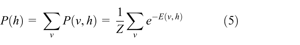
DBN model is stacked by the restricted Boltzmann machine (RBM) based on energy function.^25,26 For a given set of states (v, h), v represents the visible layer, h represents the hidden layer, and its energy function is defined as follows

E (v, h) = - \sum_{i = 1} a_{i} v_{i} - \sum_{j = 1} b_{j} h_{j} - \sum_{i = 1} \sum_{j = 1} v_{i} h_{j} ω_{ij}

(1)

where $v_{i}$ represents the ith visible layer unit, $h_{j}$ represents the jth hidden layer unit, $a_{i}$ represents the bias of the ith neurons in the visible layer, $b_{j}$ represents the bias of the jth neurons in the hidden layer, and $ω_{ij}$ represents the weight between $a_{i}$ and $b_{j}$ . The joint probability distribution P(v, h) of state (v, h) can be expressed as

P (v, h) = \frac{e^{- E (v, h)}}{Z}

(2)

Z is a normalization factor, that is, a partition function, and its expression is shown as follows

Z = \sum_{v, h} e^{- E (v, h)}

(3)

The probability distribution of v and h, namely, P(v) and P(h), also known as the likelihood function, can be expressed as follows

P (v) = \sum_{h} P (v, h) = \frac{1}{Z} \sum_{h} e^{- E (v, h)}

(4)

P (h) = \sum_{v} P (v, h) = \frac{1}{Z} \sum_{v} e^{- E (v, h)}

(5)

Assume that the state of all neurons in the visible layer is known, and the activation probability of the jth neurons in the hidden layer can be expressed as

P (h_{j} = 1 | v) = sigmoid (b_{j} + \sum_{i} v_{i} ω_{ij})

(6)

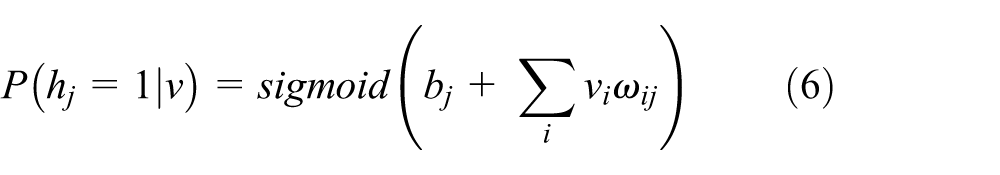
The probability of the whole hidden layer can be expressed as

P (h | v) = \underset{j}{Π} P (h_{j} | v)

(7)

Similarly, when the state of all neurons in the hidden layer is known, the activation probability of the ith neurons in the visible layer can be expressed as

P (v_{i} = 1 | h) = sigmoid (a_{i} + \sum_{j} h_{j} ω_{ij})

(8)

The probability of the whole visible layer can be expressed as

P (v | h) = \underset{i}{Π} P (v_{i} | h)

(9)

When the training sample is as follows

S = {v^{1}, v^{2}, \dots, v^{n}}

(10)

where n is the number of samples, $v^{l} (l = 1, 2, \dots, n)$ represents one of the samples, and all samples are independent and identically distributed. After the training samples are given, the RBM training process can find the optimal parameter values. Set the parameter matrix as θ = (W, a, b), the training is to maximize the following likelihood function

L (θ) = Π_{l = 1}^{n} P (v^{l})

(11)

The above formula is difficult to resolve, so it is converted to logarithmic form as follows

\ln L (θ) = \sum_{l = 1}^{n} P (v^{l})

(12)

When considering $v^{l}$ , the gradient ascent method is used to maximize the likelihood function

\frac{\partial \ln P (v^{l})}{\partial θ} = - \sum_{h} P (h | v^{l}) \frac{\partial E (v^{l}, h)}{\partial θ} + \sum_{v, h} P (v, h) \frac{\partial E (v, h)}{\partial θ}

(13)

The first item on the right side corresponds to the expectation of energy function $\partial E (v^{l}, h) / \partial θ$ under conditional distribution $P (h | v^{l})$ .

The second item on the right side corresponds to the expectation of energy function $\partial E (v, h) / \partial θ$ under conditional distribution P(v, h). Note that P(v, h) represents the joint probability distribution of the hidden layer, and it relates to the normalized Z, making this item difficult to calculate.

The contrastive divergence (CD) algorithm is used to calculate the approximate value.

The algorithm process is shown as follows:

Set the initial state of the visible layer, namely, $v^{0}$ .

Perform K-step Gibbs sampling. The t step $(t = 1, 2, \dots, k)$ is to use $P (v | h^{t - 1})$ , to perform sampling to gain $h^{t - 1}$ , and then use $P (v | h^{t - 1})$ to gain $v^{t}$ .

The approximate value of $\sum_{v, h} P (v, h) \partial E (v, h) / \partial θ$ in formula (13) can be obtained by K-step Gibbs sampling

\sum_{h} P (h | v^{k}) \frac{\partial E (v^{k}, h)}{\partial θ}

The approximate value of formula (13) can be calculated by the CD-k algorithm, and the value of the parameter matrix can be obtained. Under normal circumstances, a better result can be reached after 1-step CD algorithm.

The network parameters of DBN in each layer can be initialized during the pre-training process, achieving a better local optimum or even the global optimal region. At the highest two levels, the weights are connected together so that the output of the lower layer can associate with the top layer. DBN uses the label units to adjust the discriminant performance by means of BP algorithm. At first, the bottom-up forward propagation is carried out, and then the top-down backward propagation of multi-round supervised training is carried out. The network of proposed prediction model is shown in Figure 1.

Figure 1.

Prediction model.

As can be seen from Figure 1, DBN has a total of m layers. Vector x represents the input variables, v represents the visible layer, $(h_{1}, h_{2}, \dots, h_{m - 1})$ represents the hidden layers, and $h_{m}$ represents the output layer. The output values corresponding to vector x are set to label units, and the output values obtained by pre-training are set to top-level units. These two output values are compared with each other, and the error value between them is obtained, which is transmitted back to the input variables. According to this, the parameters of the whole prediction model are updated.

Analysis of influence factors on PV output power

There are five crucial factors found to affect the PV output power, such as solar radiation intensity, temperature, relative humidity, and wind speed. In this research, the relationship between each factor and the PV output power is formed from qualitative and quantitative study, respectively. Note that the data used in the article come from The Desert Knowledge Australia Solar Center (DKASC).

Solar radiation intensity

It is known that PV can generate the electricity power from the solar energy. The solar radiation intensity is defined as the amount of solar radiation energy at per unit area in unit time, where the unit is W m⁻². In order to verify the effect of solar radiation intensity on the output power, the data in different two days between 9 February 2015 and 13 May 2015 were collected, and the solar radiation intensity varies differently in these two days. The curves of radiation intensity and output power indicate their rough linear relationship, as shown in Figure 2(a) and (b).

Figure 2.

(a) Curves of radiation intensity and (b) output power.

Figure 2 proves that the correlation between the solar radiation intensity and output power is very high. Therefore, the solar radiation intensity is regarded as one of the main factors that affect the PV output power.

Atmospheric temperature

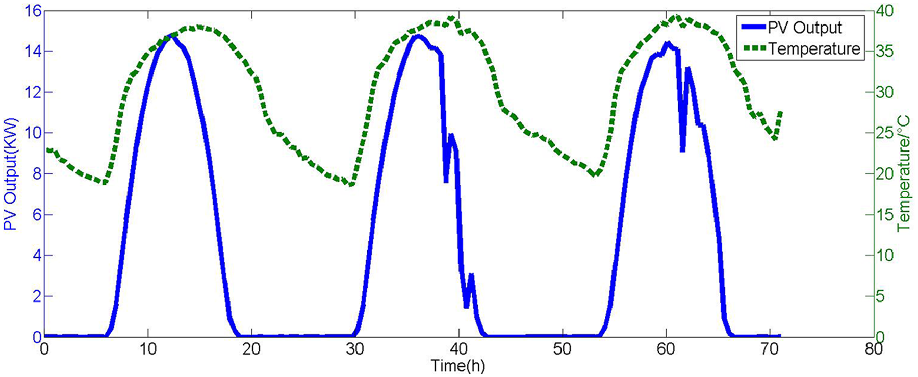
The physical quantity of atmospheric temperature can affect the PV conversion efficiency. When the air temperature is relatively high, the reduction of PV output voltage is greater than the increasing of the output current. This phenomenon results in relatively low output power, and therefore, the PV conversion efficiency becomes relatively low. Considering that the variation of the solar radiation intensity in adjacent days is little, the historical data of the atmospheric temperature and output power between 9 February 2015 and 11 February 2015 time period are selected, thus eliminating the influence of radiation intensity on output power, and the corresponding curves of atmospheric temperature and output power are shown in Figure 3.

Figure 3.

Curves of atmospheric temperature and output power.

In Figure 3, it can be seen that there is a slightly positive correlation between the atmospheric temperature curve and the output power curve. In fact, the local maximum point of the atmospheric temperature curve does not correspond to that of the output power in the PV system.

Relative humidity

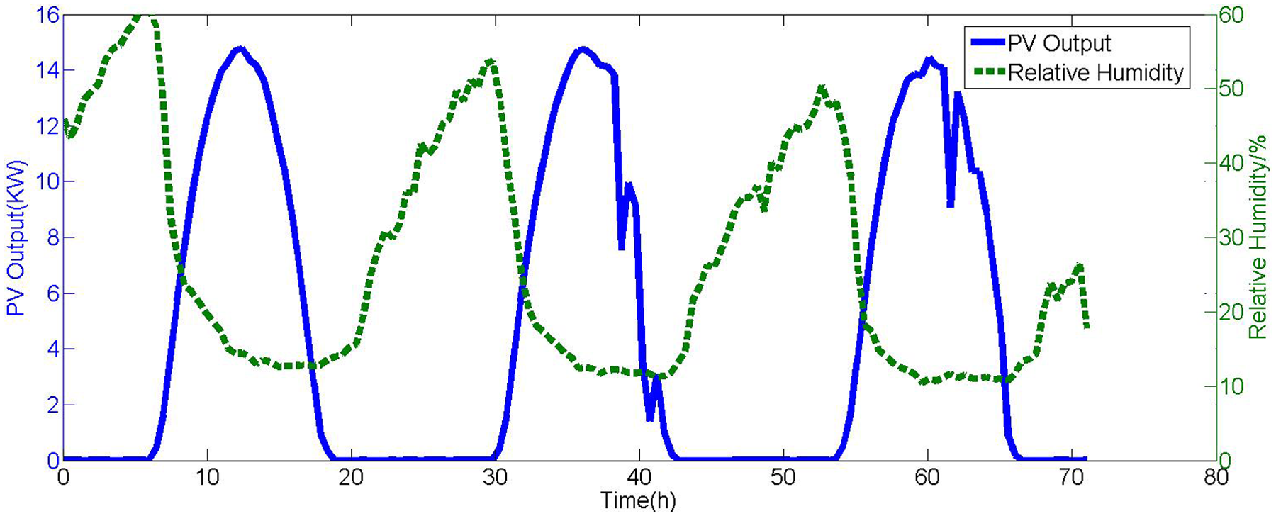
The percentage between water vapor pressure and saturated vapor pressure under the same temperature is called the relative humidity of the air. The relative curves between relative humidity and the PV output power are shown in Figure 4, where the data of the relative humidity and output power between 9 February2015 and 11 February 2015 time period were collected similarly. The results reveal that the relative humidity and PV output power are negatively correlated. It means that the solar radiation absorbed by the PV panel will be reduced when the relative humidity increases. Sequentially, the PV system output power will decrease.

Figure 4.

Curves of relative humidity and output power.

Wind speed

The wind speed can change the surface temperature of PV modules by changing the efficiency of heat transfer. In addition, the change of wind speed can also affect the clean degree of the surface of PV modules. The relative curves of wind speed and PV output power are shown in Figure 5. Similarly, the data were collected between 9 February 2015 and 11 February 2015 time period. It can be seen from Figure 5 that the volatility of wind speed curve is stronger than the output power curve. The wind speed is seen more unstable, and the correlation of the two curves is weak. So, the wind speed is regarded as an indirect factor to affect the PV output power.

Figure 5.

Curves of wind speed and output power.

Correlation coefficient between factor and the output power of PV

In this study, Pearson correlation coefficient r is used to evaluate the correlation strength between factor and the PV output power, which is defined as follows

r = \frac{\sum XY - \frac{\sum X \sum Y}{N}}{\sqrt{(X^{2} - \frac{(\sum X^{2})}{N}) (\sum Y^{2} - \frac{(\sum Y^{2})}{N})}}

(14)

where X and Y represent two data sets, and N represents the number of variables. Here, X is the PV output power, and Y is the factor that may affect the PV output power. The correlation coefficient r is located between −1 and +1, namely, |r| ≤ 1. The relation between correlation coefficient r and correlation degree is shown in Table 1.

Table 1.

Relation between correlation coefficient and correlation degree.

r	Correlation degree
−1	Completely negative
<0	Negative
0	Uncorrelated
>0	Positive
1	Completely positive

From Table 1, when $| r | \approx 1$ , the relationship between two variables is almost completely positive or negative linearity. Moreover, when |r| is closer to 1, it indicates that the linear relationship between the two variables is closer. In general, |r| < 0.2 indicates an extremely weak correlation, 0.2 ≤ |r| < 0.4 represents a low correlation, 0.4 ≤ |r| < 0.6 is a moderate correlation, 0.6 ≤ |r| < 0.8 is high correlation, and 0.8 ≤ |r| < 1 shows an extremely strong correlation. Table 2 shows the correlation results between major variables such as solar radiation intensity, air temperature, relative humidity, wind speed, and PV output power. The data were collected between 07:00 and 18:00 in 3–4 days (Figures 2 –5) in 2015.

Table 2.

Relationship of correlation coefficient and correlation degree between variables.

Item	Influence factor	r
1	Solar radiation	0.9496
2	Atmospheric temperature	0.5127
3	Relative humidity	−0.4355
4	Wind speed	0.3284

As can be seen from Table 2, the correlation between solar radiation intensity and the PV output power is strongly linear, where r = 0.9496. The correlation between the atmospheric temperature and the PV output power is moderately positive, where r = 0.5011. The relative humidity is moderately negative with the PV output power, where r = −0.4355. The correlation r = 0.3392 between the wind speed, and the PV output power is located in a low linear range, unveiling the lowest influence on the output power.

Short-term output power prediction of PV system

Determination of model inputs

Based on the above analysis, the prediction model using the DBN algorithm is established. The historical PV output power data and the physical quantity of affecting PV power are used as the input of the prediction model. The input variables in the forecasting model include the solar radiation intensity, the atmospheric temperature, and the relative humidity. These factors are proved having the mostly strong correlation with the output power. The input variables for the prediction model are shown in Table 3.

Table 3.

Input variable of prediction model.

Input variable	Variable meaning
x1	Value of solar radiation
x2	Value of atmospheric temperature
x3	Value of relative humidity
x4	Value of output power in the first day before the forecast
x5	Value of output power in the second day before the forecast
x6	Value of output power in the third day before the forecast
x7	Value of output power in the fourth day before the forecast
x8	Value of output power in the fifth day before the forecast

Data normalization

The inputs of the forecasting model contain the historical PV output power, intensity of solar radiation, air temperature, and relative humidity, where their units are kW, m s⁻², °C, and %, respectively. The input values should be normalized within the scope of [0, 1] for model implementation. Please note that the unit of relative humidity is % so that it can be normalized by dividing the value by 100 directly. The other inputs are processed as follows.

Using the following formula for normalization

\hat{x} = \frac{x - x_{min}}{x_{max} - x_{min}}

(15)

where x represents the current load value, and x_max, x_min represent the load maximum and minimum values in a day, respectively.

Prediction model evaluation

In order to verify the effectiveness of the proposed model, three functions are used to evaluate the error of output power prediction, as follows. The mean absolute percentage error (MAPE), mean squared error (MSE), and Theil’s inequality coefficient (TIC) are defined as follows

M A P E (X_{i}) = \frac{1}{l} \sum_{i = 1}^{l} | \frac{a_{i} - p_{i}}{a_{i}} | * 100 %

(16)

MSE (X_{i}) = \frac{1}{l} \sum_{i = 1}^{l} {(a_{i} - p_{i})}^{2}

(17)

TIC = \frac{\sqrt{\frac{1}{l} \sum_{1}^{l} {(p_{i} - a_{i})}^{2}}}{\sqrt{\frac{1}{l} \sum_{1}^{l} {p_{i}}^{2}} + \sqrt{\frac{1}{l} \sum_{1}^{l} {a_{i}}^{2}}}

(18)

where l represents the number of samples of the test sample set, $a_{i}$ represents the actual output power value of the i test sample set, $p_{i}$ is the prediction value of the i test sample set.

Prediction example

The data of PV output power and meteorological factors from DKASC were selected as training/test samples for two prediction models. The first group data were used for training process, being collected during 1 January 2016 to 22 February 2016 in summer and 1 March 2016 to 24 May 2016 in winter. The collection range is 9:00–17:00 and the data are collected at a frequency of one time every half an hour. Considering that the amount of solar radiation in other time periods is very small, it is not included in the study period. The second group data were used for testing process, being collected during 23 February 2016 to 29 February 2016 in summer and 25 May 2016 to 31 May 2016 in winter. A total of 17 output power values of the 9:00–17:00 for each day are predicted at intervals of half an hour, thus making the prediction time horizon 30 min, which belongs to the short-term forecasting.

Table 4 gives the weather information used for test samples, where it is derived from Meteorological Bureau of Australian Government, including air temperature, rainfall and relative humidity, and cloud information.

Table 4.

Weather information for test samples.

Date	Temperatures		Rain (mm)	9 a.m.			3 a.m.
Date	Minimum (°C)	Maximum (°C)	Rain (mm)	Temperature (°C)	RH (%)	Cld. $(8 th)$	Temp (°C)	RH (%)	Cld. $(8 th)$
25 May	11.3	29.7	0	21.5	54	0	28.9	28	0
26 May	15.3	32.0	0	24.1	50	0	31.3	28	0
27 May	17.3	22.1	0	17.5	64	8	21.0	27	0
28 May	10.2	21.2	0	14.7	47	8	20.2	29	7
29 May	11.0	27.2	0	18.7	30	0	25.9	26	2
30 May	14.1	19.6	3.0	17.3	90	8	18.8	71	6
31 May	14.2	24.1	16.8	16.6	85	3	23.3	53	7
23 February	24.6	41.1	0	35.3	16	1	39.6	12	4
24 February	23.8	42.6	0	35.3	26	1	41.1	13	6
25 February	27.7	40.9	0	33.1	26	3	39.9	17	5
26 February	22.0	34.8	26.2	27.8	41	7	34.2	29	3
27 February	20.9	35.0	0	27.2	21	1	34.2	14	2
28 February	18.6	36.2	0	27.5	22	1	35.8	13	2
29 February	18.1	36.1	0	27.9	22	0	34.9	11	1

RH: relative humidity; cld.: cloud information.

In the DBN prediction model, the number of hidden layers and the number of hidden nodes have great influence on the prediction results. Here, the hidden layer consists of three layers, and the number of nodes in each hidden layer is set to 10. To compare the results between DBN and BP algorithms, BP model used the same training samples as DBN model for prediction. The training times are set to 200. The training convergence curves from DBN and BP in February are shown in Figure 6. In the whole training process, the convergence rate of DBN is found relatively faster than BP, since the 10th time, the DBN convergent rate reaches lower error, and when the iteration is about 20 generations, the convergence curve of BP begins to converge. Besides, the training error of DBN is also smaller.

Figure 6.

Training convergent curves for both DBN and BP models.

After the training process, the test samples were used for testing process to achieve prediction. In February, for example, Figure 7 shows the error curves of the predicted results under different levels of hidden layers; it can be found that in the hidden layer number 3, the prediction error of the 7 days in February is the smallest. With the increase in the number of hidden layers, it can lead to the problem of over learning, which can reduce the prediction accuracy.

Figure 7.

Prediction error under different hidden layers in February.

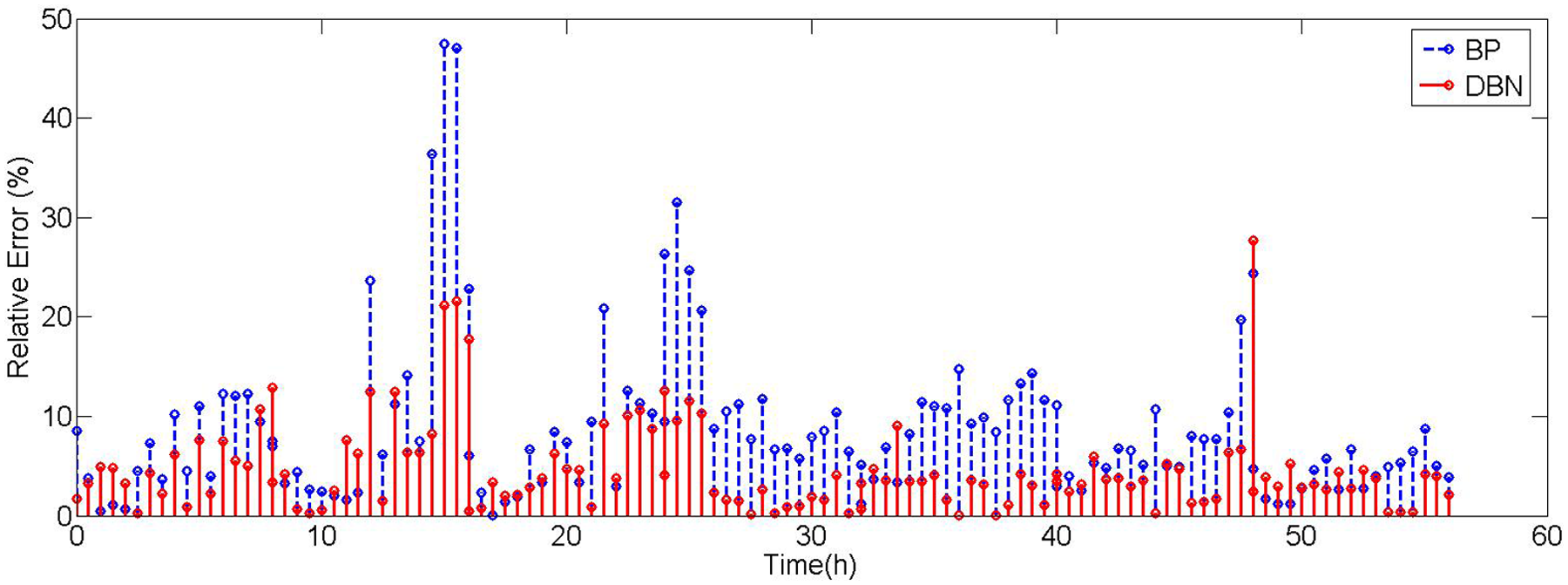
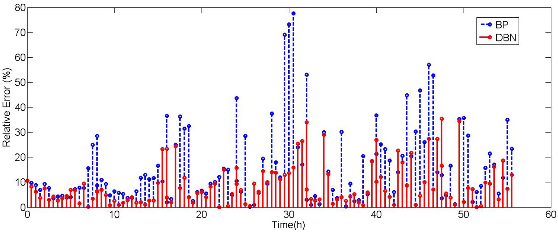
The short-term output power forecast results in May and February are shown in Figures 8 and 9, respectively. From the results, it can be seen that DBN presents better outcomes than BP. It is more obvious at the point where the output power varies significantly, but the output power is low.

Figure 8.

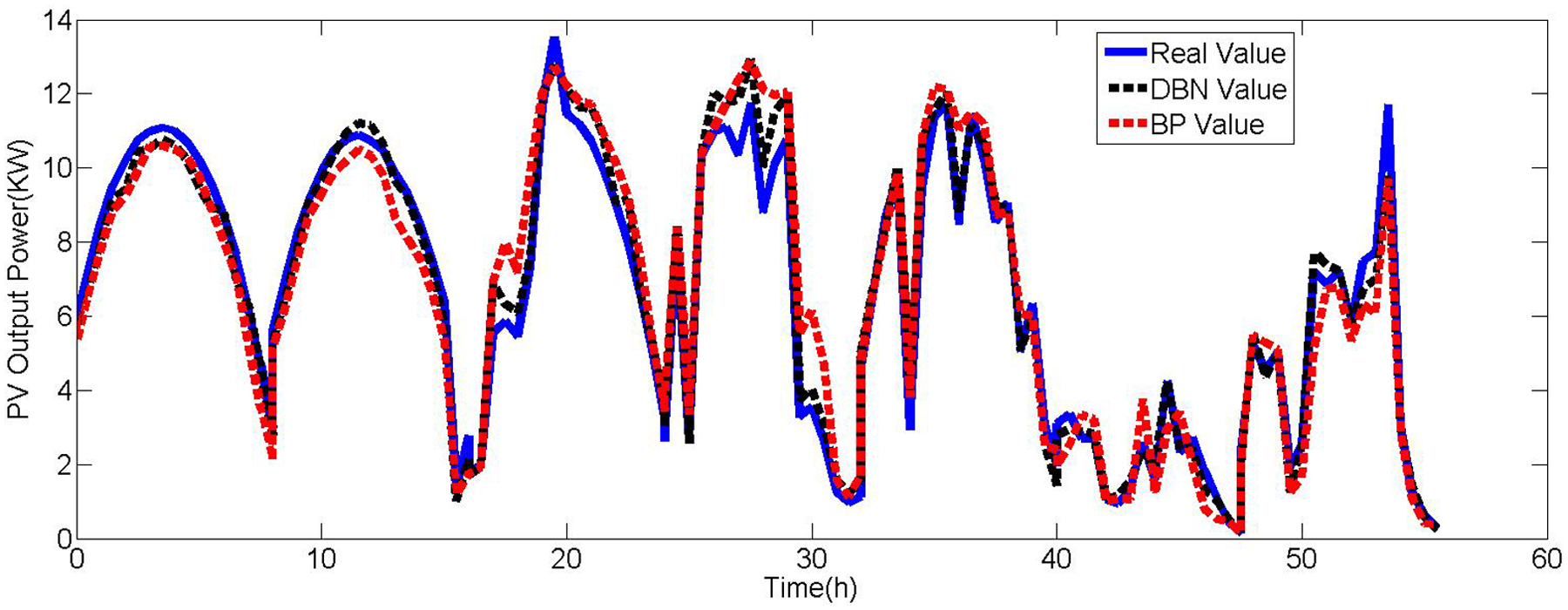
Short-term output power forecast results in May.

Figure 9.

Short-term output power forecast results in February.

In order to further verify the rationality of the proposed model, it is necessary to evaluate the prediction model. From Table 5, it can be seen that in the period of 25 May 2016 to 31 May 2016, the average errors of MAPE, MSE, and TIC obtained from the DBN prediction model are 8.92%, 0.37, and 0.039, respectively. Contrastively, the average errors of MAPE, MSE, and TIC from the BP prediction model are 16.74%, 1.00, and 0.166, respectively. It is obvious that DBN model is superior to BP model in this case. However, it is noted that the MAPE values in 28 May, 30 May, and 31 May are larger than those of other forecast days due to the cloudy and rainy weather condition. In a sunny day, the prediction error is relatively low. In other words, it is found that bad weather may increase the prediction error, especially in a rainy day. Similarly, from Table 6, it can be seen that in the period of 24 February 2016 to 29 February 2016, the average errors of MAPE, MSE, and TIC obtained by the DBN prediction model are 5.02%, 0.28, and 0.025, respectively. However, the respective values from BP model are 9.22%, 0.89, and 0.046, respectively.

Table 5.

Results of short-term output power prediction in May.

Date	DBN model			BP model
Date	MAPE (%)	MSE	TIC	MAPE (%)	MSE	TIC
25 May	5.27	0.24	0.028	9.77	0.52	0.042
26 May	5.77	0.12	0.020	10.38	0.59	0.047
27 May	7.04	0.42	0.038	13.46	1.33	0.67
28 May	13.66	0.68	0.051	29.16	2.36	0.093
29 May	7.83	0.24	0.029	10.32	0.76	0.052
30 May	13.64	0.56	0.052	27.54	0.56	0.168
31 May	9.23	0.35	0.054	16.58	0.88	0.089
Average error	8.92	0.37	0.039	16.74	1.00	0.166

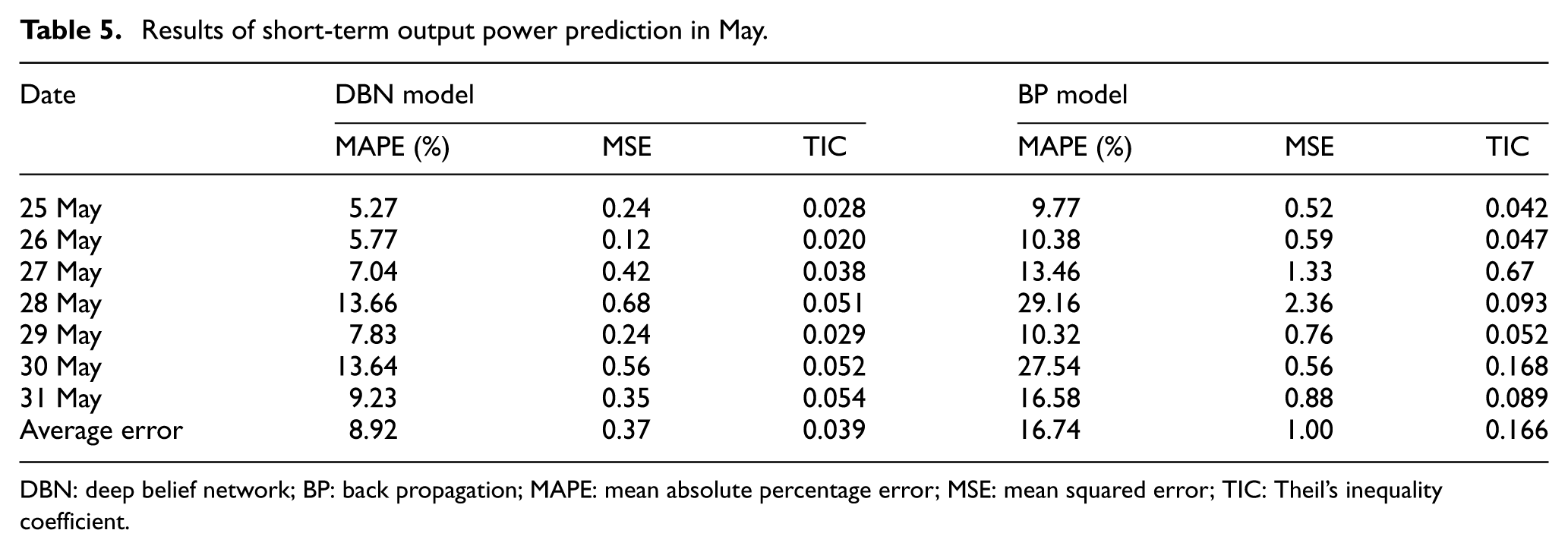
DBN: deep belief network; BP: back propagation; MAPE: mean absolute percentage error; MSE: mean squared error; TIC: Theil’s inequality coefficient.

Table 6.

Results of short-term output power prediction in February.

Date	DBN model			BP model
Date	MAPE (%)	MSE	TIC	MAPE (%)	MSE	TIC
23 February	5.18	0.31	0.027	7.11	0.70	0.041
24 February	7.84	0.51	0.037	14.24	1.07	0.054
25 February	5.22	0.34	0.030	7.06	0.66	0.041
26 February	4.45	0.23	0.023	12.51	1.55	0.061
27 February	4.11	0.20	0.021	8.89	1.06	0.050
28 February	5.05	0.19	0.020	9.65	0.89	0.046
29 February	3.31	0.15	0.019	5.11	0.31	0.027
Average error	5.02	0.28	0.025	9.22	0.89	0.046

DBN: deep belief network; BP: back propagation; MAPE: mean absolute percentage error; MSE: mean squared error; TIC: Theil’s inequality coefficient.

Comparing the predicted results with the same weather types in Tables 5 and 6, the conclusion can be drawn as follows: in the rainy day, prediction accuracy is different in the different months. According to Table 4, the rainy day of the seven forecast days in May is 30th and 31st, and 26th in February is also the rainy day of the seven forecast days in the forecast area. It can be seen that the forecast accuracy of rainy day in February is higher than that of the rainy day in May. The output power of PV system in these days will be different according to the difference of the month. The PV power generation in the forecast area is high in February, and the fluctuation is not big so that the prediction error in February is not significant. In addition, according to Table 5, 28 May is cloudy and 24th, 25th in February are the cloudy day and the sunny to cloudy day, respectively. It is found that there is difference between the forecast accuracy of different months in cloudy weather types. Besides, in sunny weather types, there is little difference between prediction accuracy and different months; however, according to the difference of the month, the situation of PV power generation is diverse, as can be seen in Figures 8 and 9, 27 May and 29 May belong to sunny weather, the output power has a certain fluctuation, so compared to other sunny forecast days, the forecast accuracy of these two days is slightly increased.

The relative error (RE) is used for the comparison of prediction accuracy evaluation between different months, which is defined as follows

R E = \frac{| a_{i} - p_{i} |}{p_{i}} * 100 %

(19)

$a_{i}, p_{i}$ represent the same parameters as equations (16)–(18). Figures 10 and 11 show prediction error curves in February and May, respectively. Their unit of horizontal axis represents the forecast time from morning 9 a.m. to 11 p.m. with intervals of half an hour in each month. In each figure, it can be seen that the RE of the prediction results gained from DBN is maintained in a reasonable range, and the stability of the prediction results is better than BP. Comparing Figure 10 with 11, another conclusion can be drawn. In May, a slight fluctuation of the REs occurs in rainy and cloudy day, and the fluctuation in February is smaller than those in May. Under the sunny weather type, there is little difference between the forecast accuracy of different months.

Figure 10.

Prediction error curves in February.

Figure 11.

Prediction error curves in May.

Conclusion

Currently, PV has been an important power generation resource in the electric power industry even though it may affect the power grid due to the inherent instability in nature. This proposed DBN prediction model for short-term output power forecasting has been performed successfully. The crucial contributions are concluded as follows.

The correlation strength between five major factors and the PV output power has been achieved, more details shown in Table 2. It indicates that the solar radiation intensity is highly correlated with the output power, and both the atmospheric temperature and relative humidity are significantly correlated. However, the relative humidity is negatively correlated, and the wind speed shows a low linear correlation.

During the 2-week prediction tests, MAPE is reduced to 7.82% and 4.2% by comparing DBN with BP in May and February, respectively. Contrastively, MSE is reduced to 0.63 and 0.61, respectively, and TIC is reduced to 0.127 and 0.021, respectively. It is obvious that the proposed DBN model for forecasting the short-term output power is superior to the BP model.

In the sunny weather, the forecast accuracy shows no significant difference in different months, having a high reliability. Contrarily, under the condition in a rainy or cloudy weather, the prediction accuracy changes considerably and causes a low reliability. This finding proves that the weather condition does affect the prediction results.

Cloudy and rainy weather have a big influence on prediction accuracy, causing an increase of the prediction error. However, sunny weather condition with small fluctuation can produce a high output power and reach a small prediction error.

Footnotes

Academic Editor: Kuei Hu Chang

Declaration of conflicting interests

The author(s) declared no potential conflicts of interest with respect to the research, authorship, and/or publication of this article.

Funding

The author(s) disclosed receipt of the following financial support for the research, authorship, and/or publication of this article: This work was supported by the National Science and Technology Supporting Plan of China (No. 2015BAA09B01), the Science and Technology Plan of Hebei Province of China (No. 14214503D), the Program of Tianjin Science and Technology Commissioner of China (No. 16JCTPJC50700), and the Colleges and Universities in Hebei Province Science and Technology Research Youth Fund (No. QN2015111).

References

Liu

Basic issues of the utilization of large-scale renewable power with high security and efficiency. Proc CSEE 2013; 33: 1–8.

Shen

Cao

Research on the influence of distributed power grid for distribution network. Trans China Electrotechnic Soc 2015; 30: 346–351.

Ding

Wang

et al . A review on the effect of large-scale PV generation on power systems. Proc CSEE 2014; 34: 1–14.

Zhao

Lei

et al . Overview of large-scale grid-connected photovoltaic power plants. Autom Electr Power Syst 2011; 35: 101–107.

Cui

Wang

et al . Research of interaction of distributed PV system with multiple access points and distribution network. Power Syst Protect Contr 2015; 43: 91–97.

Capizzi

Napoli

Bonanno

Innovative second-generation wavelets construction with recurrent neural networks for solar radiation forecasting. IEEE T Neur Net Lear 2012; 23: 1805–1815.

Shah

ASBM

Yokoyama

Kakimoto

High-precision forecasting model of solar irradiance based on grid point value data analysis for an efficient photovoltaic system. IEEE T Sustain Energ 2015; 6: 474–481.

Licciardi

Dambreville

Chanussot

et al . Spatiotemporal pattern recognition and nonlinear PCA for global horizontal irradiance forecasting. IEEE Geosci Remote S 2015; 12: 284–285.

Yona

Senjyu

Funabashi

et al . Determination method of insolation prediction with fuzzy and applying neural network for long-term ahead PV power output correction. IEEE T Sustain Energ 2013; 4: 527–523.

10.

Zhang

Beaudin

Taheri

et al . Day-ahead power output forecasting for small-scale solar photovoltaic electricity generators. IEEE T Smart Grid 2015; 6: 2253–2263.

11.

Yang

Thatte

Xie

Multitime-scale data-driven spatio-temporal forecast of photovoltaic generation. IEEE T Sustain Energ 2015; 6: 104–112.

12.

Chen

Duan

Cai

et al . Short-term photovoltaic generation forecasting system based on fuzzy recognition. Trans China Electrotechnic Soc 2011; 26: 83–89.

13.

Zhang

et al . Power system short-term load forecasting based on improved random forecast with gray relation projection. Autom Electr Power Syst 2015; 39: 50–55.

14.

Wan

Zhao

Song

et al . Photovoltaic and solar power forecasting for smart grid energy management. CSEE J Power Energ Syst 2015; 1: 38–46.

15.

Fidan

Hocaoglu

Gerek

ON.

Harmonic analysis based hourly solar radiation forecasting model. IET Renew Power Gen 2015; 9: 218–227.

16.

Tascikaraoglu

Sanandaji

Chicco

et al . Compressive spatio-temporal forecasting of meteorological quantities and photovoltaic power. IEEE T Sustain Energ 2016; 7: 1295–1305.

17.

Liu

Fang

Zhang

et al . An improved photovoltaic power forecasting model with the assistance of aerosol index data. IEEE T Sustain Energ 2015; 6: 434–442.

18.

Giorgi

Grazia

Congedo

et al . Photovoltaic power forecasting using statistical methods: impact of weather data. IET Sci Meas Technol 2014; 8: 90–97.

19.

Zhong

Tan

Zhang

et al . PV power short-term forecasting model based on the data gathered from monitoring network. China Commun 2014; 11: 61–69.

20.

Shi

Lee

W-J

Liu

et al . Forecasting power output of photovoltaic systems based on weather classification and support vector machines. IEEE T Ind Appl 2012; 48: 1064–1069.

21.

Jang

Bae

Park

H-S

et al . Solar power prediction based on satellite images and support vector machine. IEEE T Sustain Energ 2016; 7: 1255–1263.

22.

Liu

Luo

Research and development on Boltzmann machine. J Comput Res Dev 2014; 51: 1–16.

23.

Zhang

Chen

Gan

et al . Predictive deep Boltzmann machine for multiperiod wind speed forecasting. IEEE T Sustain Energ 2015; 6: 1416–1425.

24.

Hirata

Kuremoto

Obayashi

Time series prediction using DBN and ARIMA. In: Proceedings of the 2015 international conference on computer application technologies, Matsue, Japan, 31 August–2 September 2015, pp.24–29. New York: IEEE.

25.

Bengio

Chapados

Delalleau

et al . Detonation classification from acoustic signature with the restricted Boltzmann machine. Comput Intell 2012; 28: 261–288.

26.

Philip Chen

Zhang

C-Y

Chen

et al . Fuzzy restricted Boltzmann machine for the enhancement of deep learning. IEEE T Fuzzy Syst 2015; 23: 2163–2173.

Short-term output power forecasting of photovoltaic systems based on the deep belief net

Abstract

Keywords

Introduction

DBN

Analysis of influence factors on PV output power

Solar radiation intensity

Atmospheric temperature

Relative humidity

Wind speed

Correlation coefficient between factor and the output power of PV

Short-term output power prediction of PV system

Determination of model inputs

Data normalization

Prediction model evaluation

Prediction example

Conclusion

Footnotes

Declaration of conflicting interests

Funding

References