Role of viscoelasticity in non-equilibrium steady states of sheared entangled polymer mixtures

Abstract

Through two-dimensional numerical simulations, we present the detailed dynamic evolution of microstructure in sheared polymer mixtures and quantitatively analyze the role of viscoelasticity in non-equilibrium steady states. The result reveals that the viscoelastic effects play an essential role in forming a non-equilibrium steady state as well as the interfacial force, the inertial force, and the viscous force. By tuning the coefficients in a two-fluid model, we also find that the magnitude of viscoelastic contribution does influence the existence of non-equilibrium steady state.

Introduction

Since almost all systems found in nature are not in thermodynamic equilibrium, the non-equilibrium dynamics play a significant role in modern statistical physics. There are two significant classes of non-equilibrium systems: ¹ those undergo phase separation after temperature quench and those are continuously driven by applied shear force. In this article, we consider systems that contain both features—fluids undergoing phase separation in a shear flow. However, it is challenging to understand the morphological and rheological properties of these systems with both features. Early experimental^2–6 and numerical^7–12 studies revealed the basic features of non-equilibrium phase separation in binary fluids and many intriguing effects were observed, such as the highly elongated domains in very weak shear and a string phase under strong shear. There are still some discrepancies between theoretical and experimental opinions. For example, the relation $L_x~\stackrel{·}{\gamma }t{L}_y$ was predicted by theories in zero-shear systems, where the velocity field does not fluctuate.^13–15 In real fluids, however, the velocity fluctuates strongly and the hydrodynamic scaling arguments balance either interfacial and viscous or interfacial and inertial forces, ¹ leading to the power law of the form $L(t)~t^{-\alpha }$ .

Despite these previous efforts, it is still an open question whether the shear effect interrupts domain coarsening and leads to a non-equilibrium steady state independent of the system size, until Stansell’s group^1,16 provided convincing evidence for the existence of non-equilibrium steady states with finite domain size. Stansell et al. ¹ found that the sheared binary fluid mixture could attain a dynamic steady state with finite domain lengths. Besides, they also predicted a power law dependence of characteristic length $L_{\parallel }$ and $L_{\perp }$ on shear rate as $L_{\parallel }~{\stackrel{·}{\gamma }}^{-2/3}$ and $L_{\perp }~{\stackrel{·}{\gamma }}^{-3/4}$ using the Lattice Boltzmann approach. After that, Fielding ¹⁷ took a further research and found no evidence for non-equilibrium steady states in inertialess systems, which confirmed the irreplaceable role of inertia in non-equilibrium steady states.

All aforementioned studies of non-equilibrium steady states focused on binary viscous fluids with symmetric composition and ignored the role of viscoelasticity. However, most materials in the natural world exhibit some viscoelastic response, especially for those complex fluids of polymer mixtures. It is still uncertain whether these conclusions hold in viscoelastic fluids. Our recent work ¹⁸ gave a primary numerical study in binary viscoelastic fluids and revealed the existence of the viscoelastic non-equilibrium steady states. Our previous work confirmed the existence of the non-equilibrium steady states in viscoelastic fluids. However, it is unknown whether the role of viscoelastic effects is irreplaceable as the inertial. This article aims to answer this question through numerical simulations based on an extended two-fluid model. By comparing systems in pure viscous fluids of viscoelastic polymer mixture, we can identify the role of viscoelasticity. Furthermore, the magnitude of the viscoelastic contribution can be controlled by tuning the coefficients of the model; thus, we could have a quantitative analysis on it.

The remainder of this article is started by a detail description of the governing equations in section “The Flory–Huggins–Rolie–Poly fluid model.” Next section “Parameter configuration” presents the choice of the length scale and parameter sets. In section “Numerical results and discussions,” we provide numerical simulations and discussions to make a quantitative analysis. Section “Conclusion” contains the conclusions and the future work.

The Flory–Huggins–Rolie–Poly fluid model

To study the phase separation of the polymer mixture, we use an extended two-fluid model: the FH-RP (Flory–Huggins–Rolie–Poly) model, where viscoelasticity is introduced into its governing equations. Previous study has shown that FH-RP model can provide more realistic predictions of the viscoelastic responses under shear flow.^18,19 The governing equations of this model are as follows.

Consider polymer mixtures with two components, $A$ and $B$ . Let ${\varphi }_A(\overrightarrow{r},t)$ and ${\varphi }_B(\overrightarrow{r},t)$ $({\varphi }_B=1-{\varphi }_A)$ be the volume fractions of two components at point $\overrightarrow{r}$ and time $t$ , and let ${\overrightarrow{v}}_A(\overrightarrow{r},t)$ and ${\overrightarrow{v}}_B(\overrightarrow{r},t)$ be their velocities, respectively. So, the volume average velocity $\overrightarrow{v}$ is given by

$$\overrightarrow{v}={\varphi }_A{\overrightarrow{v}}_A(\overrightarrow{r},t)+{\varphi }_B{\overrightarrow{v}}_B(\overrightarrow{r},t)$$

(1)

For simplicity, we assume that the polymer mixtures are incompressible, isothermal, and viscoelastic binary fluids with equal density $\rho$ , so the motion of them is governed by the continuity equation

$$\overrightarrow{\nabla }·\overrightarrow{v}=0$$

(2)

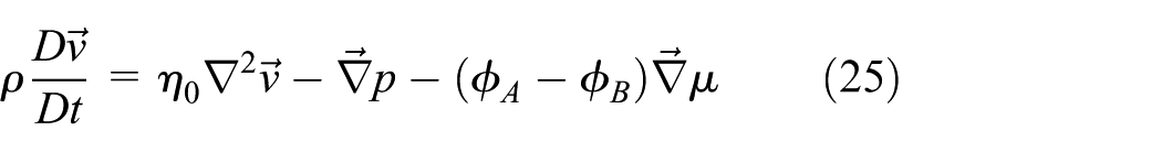
and the momentum balance equation including viscoelastic forces is

$$\rho \frac{D\overrightarrow{v}}{\mathrm{Dt}}={\eta }_0{\nabla }^2\overrightarrow{v}-\overrightarrow{\nabla }p-({\varphi }_A-{\varphi }_B)\overrightarrow{\nabla }\mu +\overrightarrow{\nabla }·{\sigma }_{\mathrm{ve}}(\overrightarrow{r},t)$$

(3)

where the material derivative is defined by $D\overrightarrow{v}/\mathrm{Dt}=(\partial \overrightarrow{v}/\partial t)+\overrightarrow{v}·\overrightarrow{\nabla }\overrightarrow{v}$ . ${\eta }_0$ is the viscosity of the Newtonian stress and $p$ is the pressure field.

$\overrightarrow{\nabla }·{\mathbf{\sigma }}_{\mathrm{ve}}(\overrightarrow{r},t)$ and $\overrightarrow{\nabla }\mu$ are two significant contributions for the momentum balance equation. $\overrightarrow{\nabla }·{\mathbf{\sigma }}_{\mathrm{ve}}(\overrightarrow{r},t)$ is the viscoelastic stress term originating from the polymer chain dynamics, and $\overrightarrow{\nabla }\mu$ is the osmotic stress term where $\mu ={\mu }_A-{\mu }_B$ represents the chemical potential difference describing the thermodynamic effects. Since the chemical potentials are approximated as defined in the Ginzburg–Landau scheme, ²⁰ we assume the chemical potential difference $\mu$ as the functional derivative of the mixing free energy with respect to local volume fraction

$$\mu =\frac{\delta {\mathcal{F}}_{\mathrm{mix}}\left[{\varphi }_A\left(\overrightarrow{r}\right)\right]}{\delta {\varphi }_A\left(\overrightarrow{r}\right)}=-\frac{\delta {\mathcal{F}}_{\mathrm{mix}}\left[{\varphi }_B\left(\overrightarrow{r}\right)\right]}{\delta {\varphi }_B\left(\overrightarrow{r}\right)}$$

(4)

A first-order approximation of the mixing free energy function is given by the Flory–Huggins–de Gennes form as

$${\mathcal{F}}_{\mathrm{mix}}\left[{\varphi }_A\left(\overrightarrow{r}\right)\right]=\int d\overrightarrow{r}\{f_{\mathrm{mix}}+\left(\frac{\Gamma }{2}\right){[\nabla {\varphi }_A]}^2\}$$

(5)

and

$$\begin{array}{c}{f}_{\mathrm{mix}}=k_{B}T[\left(\frac{1}{M_A}\right){\varphi }_A\ln {\varphi }_A+\left(\frac{1}{M_B}\right){\varphi }_B\ln {\varphi }_B+\chi {\varphi }_A{\varphi }_B]\hfill \end{array}$$

(6)

where $\Gamma$ is the interfacial tension coefficient, $M_i$ is the molecular weight of each component polymer, and $\chi$ is the Flory–Huggins interaction parameter. Therefore, we can get the potential difference by substituting equation (5) into equation (4)

$$\mu =\frac{\partial f_{\mathrm{mix}}}{\partial {\varphi }_A}-\Gamma {\nabla }^2{\varphi }_A$$

(7)

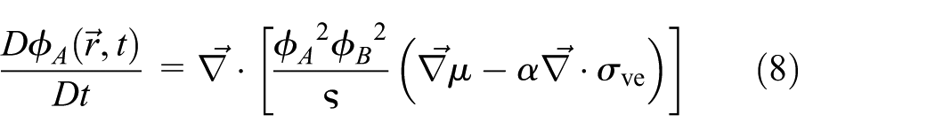
Combining the osmotic stress term with viscoelastic stress term, we get the evolution equation for the volume fraction

$$\frac{D{\varphi }_A(\overrightarrow{r},t)}{\mathrm{Dt}}=\overrightarrow{\nabla }·\left[\frac{{{\varphi }_A}^2{{\varphi }_B}^2}{\varsigma }(\overrightarrow{\nabla }\mu -\alpha \overrightarrow{\nabla }·{\sigma }_{\mathrm{ve}})\right]$$

(8)

where $\varsigma$ is a frictional coefficient. $\alpha$ is a dimensionless coefficient which is expressed by the ratio of relaxation times in Jupp and Yuan’s ²¹ model. Different from their model, we use the ratio of the entanglements number to express $\alpha$ for the polymer inhomogeneity

$$\alpha =\frac{1-G\prime Z\prime }{{\varphi }_A+G\prime Z\prime {\varphi }_B}$$

(9)

where $G\prime =G_B/G_A$ is the ratio of the modulus where $G_i(i=A,B)$ is the relaxation modulus of polymer linear blend. $G_i=G_R^i+G_d^i(i=A,B)$ , where $G_R^i$ describes the high-frequency polymer relaxation (Rouse process) and $G_d^i$ describes the disentanglement process of the chains. $Z\prime =Z_B/Z_A$ is the ratio of the entanglements number, where $Z_i=M_i/M_e^i(i=A,B)$ is the number of entanglements of each component polymer. $Z_i$ can be calculated by Rouse relaxation time ${{\tau }_R}^i$ and disentanglement relaxation time ${{\tau }_d}^i$ as $Z_i={{\tau }_d}^i/(3{\tau }_R^i)$ .

The value of $\alpha$ indicates the magnitude of the viscoelastic contribution, so we could tune the value of $\alpha$ to have a quantitative analysis on the viscoelastic contribution for non-equilibrium steady states. Especially, $\alpha$ vanishes for $G\prime Z\prime =1$ , which includes the special case of a rheologically homogeneous system, where $G\prime =1$ and $Z\prime =1$ . Besides, the sign of $\alpha$ can make the viscoelastic force term either oppose or reinforce the thermodynamics as equation (8) shows. Considering $\alpha$ varies with ${\varphi }_A$ and ${\varphi }_A$ varies with time at point $\overrightarrow{r}$ , here, we use the initial value of $\alpha$ , namely, ${\alpha }^0$ , to describe the magnitude of viscoelastic contribution in the following text.

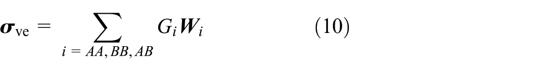
As for viscoelastic stress ${\mathbf{\sigma }}_{\mathrm{ve}}$ , it can be calculated by the sum of three parts, the contribution of the component A, component B, and the interaction between A and B

$${\mathbf{\sigma }}_{\mathrm{ve}}=\sum _{i=\mathrm{AA},\mathrm{BB},\mathrm{AB}}{G}_i{\mathit{W}}_i$$

(10)

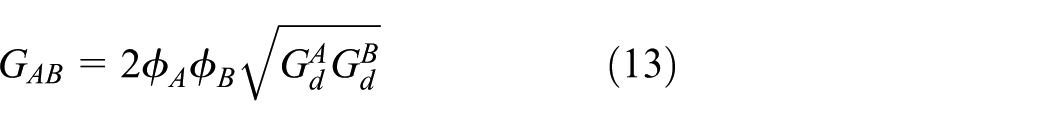
where the quantity ${\mathit{W}}_i$ is the polymer conformation tensor and parameterized by the elastic modulus $G_i$ . By applying the linear rule to the Rouse process and the “double reputation” rule to the disentanglement process, the elastic modulus of the three parts can be expressed as

$$G_{\mathrm{AA}}={\varphi }_A{G}_R^A+{{\varphi }_A}^2{G}_d^A$$

(11)

$$G_{\mathrm{BB}}={\varphi }_B{G}_R^B+{{\varphi }_B}^2{G}_d^B$$

(12)

$$G_{\mathrm{AB}}=2{\varphi }_A{\varphi }_B\sqrt{G_d^A{G}_d^B}$$

(13)

Corresponding relaxation time in $G_{i}i=\mathrm{AA},\mathrm{BB},\mathrm{AB}$ can be expressed as ${\tau }_d^{\mathrm{AA}}={\tau }_d^A$ , ${\tau }_d^{\mathrm{BB}}={\tau }_d^B$ , and ${\tau }_d^{\mathrm{AB}}=2{\tau }_d^A{\tau }_d^B/({\tau }_d^A+{\tau }_d^B)$ . For the Rouse time, there is no interacting part, so ${\tau }_R^{\mathrm{AA}}={\tau }_R^A$ , ${\tau }_R^{\mathrm{BB}}={\tau }_R^B$ , and ${\tau }_R^{\mathrm{AB}}=0$ .

According to the Rolie–Poly constitutive model, the conformation tensor ${\mathit{W}}_i$ can be calculated by solving the Rolie–Poly constitutive equations as below ²²

$$\begin{array}{c}\multicolumn{1}{c}{\frac{D{\mathit{W}}_i}{\mathrm{Dt}}=2D+{(\nabla {\overrightarrow{v}}_T)}^T·{\mathit{W}}_i+{\mathit{W}}_i·(\nabla {\overrightarrow{v}}_T)}\\ \multicolumn{1}{c}{-\frac{1}{{\tau }_d^i}{\mathit{W}}_i-f_1^i(I+{\mathit{W}}_i+f_2^i{\mathit{W}}_i)}\end{array}$$

(14)

The tube velocity $\overrightarrow{\nabla }{\overrightarrow{v}}_T$ should be used in the viscoelastic constitutive equation, ²¹ such as equation (14), rather than $\overrightarrow{\nabla }\overrightarrow{v}$ . The tube velocity ${\overrightarrow{v}}_T$ is expressed in terms of the volume average velocity as

$${\overrightarrow{v}}_T=\overrightarrow{v}+{\varphi }_A{\varphi }_B\alpha ({\overrightarrow{v}}_A-{\overrightarrow{v}}_B)$$

(15)

and the velocity difference between the two components depends on the thermodynamic and viscoelastic forces

$${\overrightarrow{v}}_A-{\overrightarrow{v}}_B=\frac{{\varphi }_A{\varphi }_B}{\varsigma }[-\overrightarrow{\nabla }\mu +\alpha \overrightarrow{\nabla }·{\mathbf{\sigma }}_{\mathrm{ve}}]$$

(16)

As for other terms in equation (14), D is defined by

$$D=\frac{1}{2}(\nabla {\overrightarrow{v}}_T+{(\nabla {\overrightarrow{v}}_T)}^T)$$

(17)

and the material derivative, $D{\mathit{W}}_i/\mathrm{Dt}$ , is defined through the tube velocity as

$$\frac{D{\mathit{W}}_i}{\mathrm{Dt}}=\frac{\partial {\mathit{W}}_i}{\partial t}+{\overrightarrow{v}}_T·\nabla {\mathit{W}}_i$$

(18)

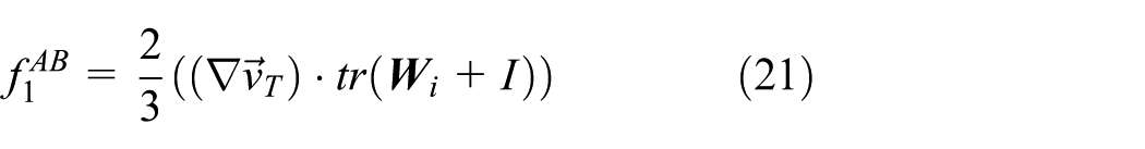
and the coefficients of the stress tensor are defined by

$$f_1^i=\frac{2}{{\tau }_R^i}(1-{(1+\frac{\mathrm{tr}\left({\mathit{W}}_i\right)}{3})}^{-1/2})\mathrm{for}i=\mathrm{AA},\mathrm{BB}$$

(19)

$$f_2^i=\beta {(1+\frac{\mathrm{tr}\left({\mathit{W}}_i\right)}{3})}^{\delta }\mathrm{for}i=\mathrm{AA},\mathrm{BB}$$

(20)

for ${\mathit{W}}_{\mathrm{AB}}$ , as ${\tau }_R^{\mathrm{AB}}\to 0$ leading to a non-stretching limit, ²³ we obtain

$$f_1^{\mathrm{AB}}=\frac{2}{3}((\nabla {\overrightarrow{v}}_T)·\mathrm{tr}({\mathit{W}}_i+I))$$

(21)

$$f_2^{\mathrm{AB}}=\beta$$

(22)

$\mathrm{tr}({\mathit{W}}_i)$ represents the trace of the tensor ${\mathit{W}}_i$ , $\beta$ represents the CCR (convective constraint release) magnitude coefficient, and $\delta$ represents some negative power specifying the exponent for the relaxation due to the CCR. For simplicity, but without much loss of generality, we assume $\beta$ for all three parts are of the same value, so is $\delta$ .

The aforementioned equations present the FH-RP model in this article. By selecting parameter space for the FH-RP model in terms of ${\eta }_0$ , ${\tau }_R^A$ , ${\tau }_d^A$ , ${\tau }_R^B$ , ${\tau }_d^B$ , $G_R^A$ , $G_R^B$ , $G_d^A$ , $G_d^B$ $(G_A=G_R^A+G_d^A,G_B=G_R^B+G_d^B)$ , and the shear rate $\stackrel{·}{\gamma }$ , we can obtain appropriate rheology behavior in shear flow.

Parameter configuration

Our simulation is applied on the two-dimensional rectangular box with size of ${\Lambda }_x\times {\Lambda }_y$ . The top and bottom boundaries are physical walls and the other two sides are applied to periodic boundary conditions (Lees–Edwards boundary conditions) so that the shear rate $\stackrel{·}{\gamma }$ can be applied by moving the upper wall boundary to the right at a constant speed $\stackrel{·}{\gamma }{\Lambda }_y$ . To eliminate the finite-size effects, we must ensure the typical domain size $L<<{\Lambda }_{x,y}$ . In previous study,^1,15,18 the finite-size effects are under control when the system size is in the range of ${\Lambda }_x=512-2048$ and ${\Lambda }_y=256-1024$ . Thus, all simulations in this study are done for asymmetric quenches on a ${\Lambda }_x\times {\Lambda }_y=1024\times 256$ justifying both the accuracy and the efficiency.

There have been many possible measures of the characteristic length so far. For example, the structure factor based on Fourier transform is usually used to define a characteristic length in zero-shear systems, while under shear, the system is no longer periodic and the morphology will be anisotropic in general, which makes the structure factor not distinguish one Cartesian direction from another accurately. Given this, we define two orthogonal length scales $L_{\parallel }$ and $L_{\perp }$ to characterize the long and short principal axes of the domain morphology using a gradient statistic for ${\varphi }_A$ across the simulation box. They are the reciprocal eigenvalues of the symmetric matrix^1,17,24

$$D_{\alpha \beta }=\frac{l\int \mathrm{dx}\int \mathrm{dy}{\partial }_{\alpha }{\varphi }_A{\partial }_{\beta }{\varphi }_A}{\int \mathrm{dx}\int \mathrm{dy}{\varphi }_A^2}$$

(23)

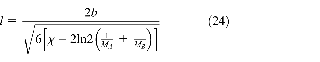
where $l$ is the width of the interface between domains and can be calculated by Helfand and Tagami’s ²⁵ self-consistent field theory.^26,27 Taking into account the finite chain length, Broseta ²⁸ and Schubert ²⁹ predicted a broader interface and smaller interfacial tension. According to our simulation observations, Broseta’s formulation gave a more accurate description of the interfaces as

$$l=\frac{2b}{\sqrt{6[\chi -2\ln 2(\frac{1}{M_A}+\frac{1}{M_B})]}}$$

(24)

where $\chi$ is the Flory–Huggins interaction parameter in equation (5) and the statistical segment length $b$ is given in terms of the interfacial tension coefficient $\Gamma$ as $b=\sqrt{18\Gamma }$ . ³⁰

For a convincing conclusion and free of finite-size effects, the characteristic length should be larger than the mesh size and much smaller than the system size. Therefore, in any given run, we must ensure the separation of the length scales

$${\delta }_{x,y}<<l<<L_{\parallel ,\perp }<<{\Lambda }_{x,y}$$

(24)

where ${\delta }_x={\delta }_y=1$ is the mesh size of the simulation box. Our previous study finds it difficult to restrict the $L_{\perp }$ significant larger than the mesh size, while this defect has been made up in this study.

For simplicity, but without loss of generality, we set the following parameters as ${\eta }_0=0.1$ , $M_A=M_B=1$ , $k_{\mathrm{B}}T=1.3$ , $\Gamma =1$ , $\varsigma =0.1$ , $\rho =1$ , $\beta =0.2$ , and $\delta =-0.5$ . As for the interaction parameter $\chi$ and the initial volume fraction ${{\varphi }_A}^0$ , the $\chi /{\varphi }_A^0$ parameter space of a Flory–Huggins fluid is shown in the equilibrium phase diagram Figure 1. In this diagram, $\partial f_{\mathrm{mix}}/\partial {\varphi }_A=0$ defines the binodal curve and is shown as the broken line. Below this, the system favors a homogeneous state in equilibrium. ${\partial }^2{f}_{\mathrm{mix}}/\partial {\varphi }_A^2=0$ defines the spinodal curve and is shown as the solid line. For $({\varphi }_A^0,\chi )$ above the spinodal (solid) line, homogeneous states are unstable and systems will spontaneously decompose into two coexisting phases. There is the critical point at $({\varphi }_A^0=0.5,\chi =2)$ in the diagram. By changing the values of $\chi$ and ${\varphi }_A^0$ , we can explore different regions of the phase diagram.

Figure 1.

Equilibrium phase diagram with parameter set as $M_A=M_B=1.0$ and $k_{B}T=1.3$ . Areas of homogeneous and two-phase fluids are bordered by binodal and spinodal lines. A metastable region is between the lines. The point marked by the bold cross is $({\varphi }_A^0,\chi )=(0.3,3.0)$ .

Focusing on the binary polymer mixtures with asymmetric composition, we choose the point $(0.3,3.0)$ as the fixed values of ${\varphi }_A$ and $\chi$ , respectively, which is marked as the bold cross in the figure. This point is in the two-phase region where the spontaneous decomposition will take place with infinitesimal amplitude non-local fluctuations of composition. Thus, we superimpose Gaussian noise with an intensity of ${10}^{-3}$ onto the initial uniform composition field ${\varphi }_A^0$ in all simulations in order to obtain the phase separation of the fluids.

So far, the essential system size ( ${\Lambda }_x,{\Lambda }_y$ ), characteristic length ( $L_{\parallel },L_{\perp }$ ), and constants ( ${\eta }_0,M_A,M_B,k_{\mathrm{B}}T,\Gamma ,\varsigma ,\rho ,\beta ,\delta$ ) have been set. Other parameters are listed in Table 1, where the values of ${\tau }_R^A$ and ${\tau }_R^B$ vary from each case. According to equation (9), the value of ${\alpha }^0$ depends on ${{\tau }_R}^i$ and ${{\tau }_d}^i(i=A,B)$ , so ${\alpha }^0$ varies from each case. Different from the fixed value of ${\alpha }^0$ in our previous study, ¹⁸ we tune the value of ${\alpha }^0$ in order to find the effect of magnitude of viscoelastic contribution on the non-equilibrium steady states.

Table 1.

Parameter sets used in simulations.

Name	${\tau }_R^A$	${\tau }_d^A$	$G_A$	${\tau }_R^B$	${\tau }_d^B$	$G_B$	$Z\prime$	${\alpha }^0$
R000	–	–	–	–	–	–	–	–
R001	1	30	2.5	1	5	2.5	0.1667	2.0
R002	4.5	60	2.5	2	10	2.5	0.375	1.111
R003	2.472	30	2.5	1	5	2.5	0.412	1.0
R004	7	30	2.5	2	5	2.5	0.5833	0.588
R005	3.777	30	2.5	1	5	2.5	0.6295	0.5
R006	4	30	2.5	1	5	2.5	0.667	0.43
R007	4.5	30	2.5	1	5	2.5	0.75	0.3
R008	5.4	30	2.5	1	5	2.5	0.9	0.1
R009	3	30	2.5	0.5	5	2.5	1	0
R010	6.648	30	2.5	1	5	2.5	1.108	–0.1
R011	1.062	30	2.5	0.1	5	2.5	1.769	–0.5
R012	1.5	30	2.5	0.1	5	2.5	2.5	–0.73
R013	1	3	2.5	0.1	1.3	2.5	4.333	–1

In Table 1, R000 is a special case in pure viscous fluid without viscoelasticity, whose governing equations stem from Navier–Stokes equation and Cahn–Hilliard equation and have no viscoelastic terms. Here are governing equations of R000

$$\rho \frac{D\overrightarrow{v}}{\mathrm{Dt}}={\eta }_0{\nabla }^2\overrightarrow{v}-\overrightarrow{\nabla }p-({\varphi }_A-{\varphi }_B)\overrightarrow{\nabla }\mu$$

(25)

$$\frac{D{\varphi }_A(\overrightarrow{r},t)}{\mathrm{Dt}}=\overrightarrow{\nabla }·\left[\frac{{{\varphi }_A}^2{{\varphi }_B}^2}{\varsigma }\left(\overrightarrow{\nabla }\mu \right)\right]$$

(26)

which are different from the equations of R009. Although $\alpha =0$ in R009, the viscoelastic stress term $\overrightarrow{\nabla }·{\mathbf{\sigma }}_{\mathrm{ve}}(\overrightarrow{r},t)$ is still in momentum balance equation (3).

Since high shear rate gives inaccuracies and low shear rate gives unacceptably long run times, ¹ we set a window of shear rates $1.95\times {10}^{-3}\le \stackrel{·}{\gamma }\le 2.93\times {10}^{-2}$ for asymmetric quench according to our previous work. ¹⁸

Numerical results and discussions

In this article, we use an iterative solution algorithm based on pressure implicit split operator (PISO) algorithm to solve the FH-RP model. Recently, this algorithm has been well tested in our previous study of shear-banding flow with a macroscopic two-fluid model. ¹⁹ The governing equations of the FH-RP model are discretized through finite volume method, which locally satisfied the physical conservation laws through computing each term of the governing equations by the integral over a control volume. In this article, we use an open source computational fluid dynamics (CFD) toolbox of OpenCFD Ltd named OpenFOAM to implement the finite volume method. For spatial discretization terms of the equation, Gauss MINMOD and Gauss linear are applied in the discretization scheme. For temporal terms, the Euler scheme is applied. After this treatment, all equations can be reduced to linear systems so that we can use the iterative solvers in OpenFOAM to get the solutions at every time step. Typical solvers in OpenFOAM include the preconditioned conjugate gradient (PCG) and preconditioned biconjugate gradient (PBICG) methods. Please refer to the OpenFOAM manual for details.

To investigate the role of viscoelasticity in non-equilibrium steady states, we first reproduce behaviors seen earlier in our previous study by running the R001 case, whose parameter sets were used in the work by Guo et al. ¹⁸ As a comparison, R000 is in pure viscous fluid without viscoelasticity, but its constant parameters ( ${\eta }_0,M_A,M_B,k_{\mathrm{B}}T,\Gamma ,\varsigma ,\rho ,\beta ,\delta$ ) are the same as those of R001.

Since the domain morphology of shear flow is anisotropic, we need two length scales to characterize it accordingly. Figure 2 presents the plots of two characteristic lengths $L_{\parallel }$ and $L_{\perp }$ with $\stackrel{·}{\gamma }=1.992\times {10}^{-2}$ for R000 and R001. From Figure 2(a), we can find that $L_{\parallel }$ of R001 saturates for a long time and shows temporal fluctuations on mean values. With $L_{\parallel }{,}_{\perp }\le {\Lambda }_{x,y}/6$ , we may conclude that the finite-size effects in R001 are fully under control.

Figure 2.

Plots of $L_{\parallel }$ and $L_{\perp }$ for R000 and R001 with $\stackrel{·}{\gamma }=1.992\times {10}^{-2}$ . R001 reaches a steady state after $\stackrel{·}{\gamma }t=60$ . Yet there is no evidence of the non-equilibrium steady states with finite domain size in R000, for $L_{\parallel }$ of R000 increases indefinitely: (a) larger characteristic length $L_{\parallel }$ versus strain $\stackrel{·}{\gamma }t$ and (b) smaller characteristic length $L_{\perp }$ versus strain $\stackrel{·}{\gamma }t$ .

Snapshots of morphologies for R001 are presented in Figure 3, which show the process of phase transition from an initial homogeneous state for R001 in detail. At $\stackrel{·}{\gamma }t=11.95$ , the system has formed a two-phase state, where droplet patterns are rapidly stretched along the flow direction. From $\stackrel{·}{\gamma }t=11.95$ to $\stackrel{·}{\gamma }t=119.52$ , the morphology is becoming coarser and coarser through diffusive mechanism. At late times $\stackrel{·}{\gamma }t=119.52$ and $\stackrel{·}{\gamma }t=149.4$ , the structures of composition field ${\varphi }_A$ are highly elongated, and the continuous stretching and breaking lead to slower domain growth than the diffusive regime. After a long time, the system reached a dynamic steady state at $\stackrel{·}{\gamma }t=268.92$ . Phase transitions from visual observations for composition field ${\varphi }_A$ suggest that the length saturation stems from hydrodynamic balance between the stretching, breaking, and the coalescence of domain. Combined with plots in Figure 2, we can confirm that the system in R001 has attained a non-equilibrium steady state with finite domain size.

Figure 3.

Snapshots of domain morphologies at various strains $\stackrel{·}{\gamma }t$ . Results are obtained under applied shear rate $\stackrel{·}{\gamma }=1.992\times {10}^{-2}$ with parameter set R001: (a) $\stackrel{·}{\gamma }t=11.95$ , (b) $\stackrel{·}{\gamma }t=119.52$ , (c) $\stackrel{·}{\gamma }t=149.4$ , and (d) $\stackrel{·}{\gamma }t=268.92$ .

However, the result in R000 is totally different from that in R001. The plot of R000 in Figure 2(a) shows that $L_{\parallel }$ perpetually increases without bound. Morphologies of R000 are presented in Figure 4. Initially, the scattered droplets are rapidly elongated along the flow direction at $\stackrel{·}{\gamma }t=11.95$ ; after $\stackrel{·}{\gamma }t=119.52$ , the domain has formed into extremely long string patterns and appears to stretch indefinitely until the domain size attains the system size, which is similar to the experimental observations under strong shear.^2,4 Thus, there is no evidence of non-equilibrium steady states free of finite-size effects in R000.

Figure 4.

Snapshots of domain morphologies at various strains $\stackrel{·}{\gamma }t$ . Results are obtained under applied shear rate $\stackrel{·}{\gamma }=1.992\times {10}^{-2}$ with parameter set R000: (a) $\stackrel{·}{\gamma }t=11.95$ , (b) $\stackrel{·}{\gamma }t=119.52$ , (c) $\stackrel{·}{\gamma }t=149.4$ , and (d) $\stackrel{·}{\gamma }t=268.92$ .

For the system in non-equilibrium state, there is hydrodynamic balance between the stretching, breaking, and coalescence of the domains through the action of shear force, diffusive, viscous, inertia, and viscoelastic dynamics (for pure viscous fluids, there are no viscoelastic dynamics). From the discussion above, it is seen that system in R000 without viscoelasticity is dominated by shear and cannot reach a non-equilibrium steady state with finite domain size. However, once viscoelasticity is introduced into the governing equations, this state can be reached in R001 with the same configuration except parameters related to viscoelastic term. This result clearly suggests that the viscoelastic dynamics may interrupt the domain stretching with diffusive, viscous, and inertia dynamics. Given that the interfacial tension, viscosity, and inertia are the same for both cases, it can be concluded that viscoelastic effects play an essential role in forming a non-equilibrium steady state as well as the interfacial, the inertial, and the viscous forces. We also test both runs in different sets of viscosity ${\eta }_0$ and density $\rho$ and get similar results.

In the aforementioned discussion, we confirm the irreplaceable role of viscoelasticity for a non-equilibrium steady state. Furthermore, we also find that not all runs with viscoelastic stress terms can reach non-equilibrium steady states. Some runs fail to reach it just because of different ${\alpha }^0$ , in other word, different viscoelastic contribution.

To study the effect of the magnitude of viscoelastic contribution, we tune the value of ${\alpha }^0$ from −1 to 2.0. As shown in Table 1, constants ( ${\eta }_0,M_A,M_B,k_{\mathrm{B}}T,\mathrm{etc}.$ ) of runs R001–R013 are of the same, but the values of ${\alpha }^0$ vary from each case. Figure 5 shows the characteristic lengths $L_{\parallel }$ and $L_{\perp }$ as a function of $\stackrel{·}{\gamma }t$ for some typical runs. It can be seen that plot of $L_{\parallel }$ in Figure 5(a) can be divided into two groups. Group A includes R001, R002, R004, and R005. Group B includes R006, R010, R011, and R013. In group A, Figure 5(a) shows decisive evidence of length scale saturation in a regime which is free of finite-size effects, while in group B, $L_{\parallel }$ in Figure 5(a) of each run seems to increase indefinitely with the growth of time, until it attains the system size. Corresponding morphologies of group A and group B are shown in Figures 6 and 7, respectively. Focusing on statistically steady state, these figures only present snapshots of composition field at $\stackrel{·}{\gamma }t=209.16$ . In Figure 6, the domain of each run has formed into numerous stretching and breaking bands as well as irregular droplets, where finite-size effects are under control. In contrast, domains in Figure 7 are elongated into some short and smooth band structures with pronounced finite-size effects. So, we can confirm that non-equilibrium steady states are attained in group A but not in group B. It is seen that only when the value of ${\alpha }^0$ is in a certain range ( ${\alpha }^0\ge 0.5$ ), the system could attain a non-equilibrium steady state. Table 2 supports this conclusion via showing the existence of non-equilibrium steady states with finite domain size for all the simulations, ordered by ${\alpha }^0$ .

Figure 5.

Plots of $L_{\parallel }$ and $L_{\perp }$ for various runs with $\stackrel{·}{\gamma }=1.992\times {10}^{-2}$ . Data sets arranged by descending order of $\alpha$ correspond to R001, R002, R004, R005, R006, R010, R011, and R013. Steady states with finite domain size are attained in R001, R002, R004, and R005, while R006, R010, R011, and R013 fail to reach it. It is seen that only when ${\alpha }^0\ge 0.5$ , the system of each run could attain a non-equilibrium steady state: (a) larger characteristic length $L_{\parallel }$ versus strain $\stackrel{·}{\gamma }t$ and (b) smaller characteristic length $L_{\perp }$ versus strain $\stackrel{·}{\gamma }t$ .

Figure 6.

Snapshots of domain morphologies at $\stackrel{·}{\gamma }t=209.16$ for various runs in group A. Results are obtained under applied shear rate $\stackrel{·}{\gamma }=1.992\times {10}^{-2}$ with parameter sets R001, R002, R004, and R005. All of the runs reach a steady state at this time: (a) R001, (b) R002, (c) R004, and (d) R005.

Figure 7.

Snapshots of domain morphologies at $\stackrel{·}{\gamma }t=209.16$ for various runs in group B. Results are obtained under applied shear rate $\stackrel{·}{\gamma }=1.992\times {10}^{-2}$ with parameter sets R006, R010, R011, and R013. Domains of all runs have formed into extremely long string-like patterns, showing no evidence of non-equilibrium steady states with finite domain size: (a) R006, (b) R010, (c) R011, and (d) R013.

Table 2.

Existence of non-equilibrium steady states with finite domain size for all the simulations, ordered by ${\alpha }^0$ .

Name	${\alpha }^0$	Y/N
R001	2.0	Y
R002	1.111	Y
R003	1.0	Y
R004	0.588	Y
R005	0.5	Y
R006	0.43	N
R007	0.3	N
R008	0.1	N
R009	0	N
R010	–0.1	N
R011	–0.5	N
R012	–0.73	N
R013	–1	N

Y/N represents whether the system attains a non-eq28 steady state.

According to equation (8), the coefficient $\alpha$ actually indicates the magnitude of viscoelastic contribution. We can thereby confirm that the magnitude of viscoelastic contribution does influence the existence of non-equilibrium steady state. We also test some other parameter set by changing the density $\rho$ or viscosity ${\eta }_0$ , which does not change the conclusions before.

Conclusion

The non-equilibrium dynamics play an essential role in mechanical engineering and are found commonly in the nature world. Based on our previous research, we numerically study the non-equilibrium steady states in binary polymer mixtures with an extended two-fluid model, the FH-RP fluid model.

Our study confirms the irreplaceable role of viscoelasticity for the first time in forming a non-equilibrium steady state. As shown in our numerical results, the system of testing case without viscoelastic stress cannot attain a non-equilibrium steady state in the given parameter configuration. However, once introducing the viscoelasticity into the governing equations, non-equilibrium steady states can be reached with the same configuration. Therefore, viscoelasticity may interrupt the domain stretching with diffusive, viscous, and inertia dynamics, resulting in a non-equilibrium steady state. This result reveals the essential role of viscoelasticity in forming a non-equilibrium steady state as well as the interfacial force, the inertial force, and the viscous force. Furthermore, our simulation results show that only when dimensionless coefficient $\alpha$ is in a certain range, the system could attain a steady state. Since this coefficient indicates the magnitude of viscoelastic contribution, we may conclude that the existence of non-equilibrium steady state depends on the magnitude of viscoelastic contribution in the system.

For future work, we aim to employ parallel optimization of numerical algorithms so that the computational costs can be significantly reduced. Besides, we will improve the scalability of the simulation programs and execute three-dimensional (3D) simulations on large-scale clusters to obtain more realistic data.