Non-equilibrium steady states of entangled polymer mixtures under shear flow

Abstract

By solving the full equations of an extended two-fluid model in two dimensions, we give the first numerical study revealing non-equilibrium steady states in sheared entangled polymer mixtures. This research provides answers for some fundamental questions in sheared binary mixtures of entangled polymers. Our results reveal that non-equilibrium steady states with finite domain size do exist, and apparent scaling exponents $L_{\parallel }~{\stackrel{·}{\gamma }}^{-1.05}$ and $L_{\perp }~{\stackrel{·}{\gamma }}^{-1}$ are found over six decades of shear rate. Since the wall effects get involved in our simulations, the dependence of average domain size on system size cannot be strictly eliminated. In addition, as an obvious influence of viscoelasticity, the polymer viscosity ${\eta }_p$ appears to induce linear translation of the fitted lines. Through two-dimensional numerical simulations, we show the detailed dynamic evolution of microstructure in binary polymer mixtures with asymmetric composition under shear flow. It is found that the phase patterns are significantly different from symmetric fluids studied previously. Finally, we also identify the importance of wall effects and confirm the irreplaceable role of inertia for a non-equilibrium steady state.

Introduction

The non-equilibrium dynamics play an essential role in the applications of numerous areas ranging from soap manufacture to biological systems; ¹ in fact, most systems found in nature are not in thermal equilibrium. One of the important problems in such systems is to understand the morphological and rheological properties of the fluids undergoing a steady shear flow after a temperature quench. Early experimental^2–6 and numerical^7–12 research revealed the basic features of non-equilibrium phase separation in binary fluids, especially for the spinodal decomposition dynamics. A number of intriguing effects induced by shear were observed; typical results included the highly elongated domains in very weak shear and a string phase in steady state under strong shear. Different from the power law of the form $L(t)~t^{-\alpha }$ in zero-shear systems, the domains become elongated in the flow direction under shear. The relation $L_x~\stackrel{·}{\gamma }{\mathrm{tL}}_y$ was predicted by theories in which the velocity field did not fluctuate.^13–15 It is found that the velocity strongly fluctuates in real fluids and the hydrodynamic effects may balance either interfacial and viscous or interfacial and inertial forces. Nevertheless, it remained unclear whether the shear effects interrupted domain coarsening and restored a non-equilibrium steady state independent of the system size, until Stansell and colleagues^16,17 answered this question by numerical study. Using lattice Boltzmann approach, they provided convincing evidences for the non-equilibrium steady states with a finite domain size and predicted a power law dependence of characteristic length $L_{\parallel }$ and $L_{\perp }$ on shear rate as $L_{\parallel }~{\stackrel{·}{\gamma }}^{-2/3}$ and $L_{\perp }~{\stackrel{·}{\gamma }}^{-3/4}$ . After that, Fielding ¹⁸ presented an in-depth numerical study on the role of inertia in non-equilibrium steady states and confirmed that the non-equilibrium steady states free of finite-size effects only existed in the systems with inertia.

All the previous studies on non-equilibrium steady states focused on the binary viscous fluids with symmetric composition and ignored the role of viscoelasticity. Since all the materials exhibit some viscoelastic response in nature and many complex fluids such as polymer mixtures display significant viscoelastic effects, it is still uncertain whether these conclusions will be maintained in viscoelastic fluids. Deep-quench experiments of Tanaka ¹⁹ have shown that the dynamics of polymer phase transitions can be very different from those of classical binary fluid mixtures. Besides, the asymmetry between the components of polymer mixtures can also strongly change the morphology of phase separation.^19,20 Typically, in the zero-shear system, an asymmetric quench can lead to a droplet pattern, other than the bicontinuous pattern for a nearly symmetric quench. ²¹

Up to now, some fundamental issues, such as the existence of the non-equilibrium steady states free of system size in binary viscoelastic fluid, the rationality for fitting the domain size versus the inverse shear rate to simple power low and the dynamic morphology for an asymmetric quench under shear flow, remain open questions. This article aims to answer these questions through a numerical study considering all the effects of thermodynamics, hydrodynamics and the viscoelasticity.

By combining the thermodynamics, hydrodynamics and viscoelasticity in a thermodynamically consistent way, the two-fluid model^22–25 was widely used to investigate the phase separation in viscoelastic fluids. Such models could be used to replace the previous simple theoretical frameworks for studying the non-equilibrium viscoelastic phase separation.

Different extended versions of the two-fluid model have been proposed for studying the flow-induced phase separation. Jupp and Yuan’s model (Flory–Huggins–Johnson–Segalman (FH–JS) model)^20,26,27 coupled the FH mixing free energy function and the JS constitutive model in a unified way. They numerically solved the full equations of the two-fluid model without simplifications used widely in early studies. Fielding and Olmsted^28,29 extended the two-fluid model using a different approach, which still retained a diffusive stress term in the JS constitutive equation. As the two-fluid model has already accounted for fluid diffusion across streamline in a thermodynamically consistent way, there are no sound physical reasons for an ad hoc mechanical diffusive term to produce numerical results more compatible with experimental observations. Cromer et al. ³⁰ coupled the concentration and the stress through a two-fluid approach to predict the steady-state shear-banding for a monodisperse polymer solution. As the JS constitutive model was known to provide unrealistic rheological predictions for entangled polymeric solutions, they replaced the constitutive equation with a tube theory–based model: the Rolie–Poly (RP) model. ³¹ Nevertheless, only one-dimensional calculations had been presented. Recently, we presented a unified model ³² (FH–RP model) based on the FH–JS framework to study the rheological instabilities in shear-banding flow. The simulation results showed that this model could capture the essential dynamic features of viscoelastic phase separation and the rheochaos reported in the literature.

In this article, we focus on studying the non-equilibrium steady states of entangled polymer mixtures using the FH–RP model and start by introducing the governing equations and the choice of the parameter sets, the length and time scales in sections ‘The FH–RP fluid model’ and ‘Length scale, time scale and parameter sets’, followed by the simulation results and discussions in section ‘Numerical results and discussions’. Section ‘Conclusion’ contains our conclusions and the future work.

The FH–RP fluid model

After Helfand and Fredrickson ³³ showed the crucial stress and concentration coupling by analysing the microscopic Rouse model, Doi and Onuki ²² and Milner ²³ derived the fundamental equations of the two-fluid model for describing the polymer solutions through a more general approach. Yuan’s and colleagues ²⁷ solved a full two-fluid model coupling the FH free energy function and the JS constitutive model. Based on the FH–JS framework, we replaced the phenomenological JS model by the molecular theory–based constitutive equation. Previous numerical results ³² have shown that this FH–RP model can capture the essential dynamic features of viscoelastic phase separation and reproduce the rheochaos without introducing extra parameters. We summarize the governing equations of the FH–RP model below.

Considering the polymer mixtures with two components, A and B. Let ${\varphi }_A(\overrightarrow{r},t)$ and ${\varphi }_B(\overrightarrow{r},t)=1-{\varphi }_A(\overrightarrow{r},t)$ be the volume fractions of the two components at some point $\overrightarrow{r}$ and time $t$ . By assuming the equal density $\rho$ of the components, we can get the continuity equation and the momentum balance equation of an incompressible, isothermal viscoelastic binary fluid as

$$\overrightarrow{\nabla }·\overrightarrow{v}=0$$

(1)

and

$$\rho \frac{D\overrightarrow{v}}{\mathrm{Dt}}={\eta }_0{\nabla }^2\overrightarrow{v}-\overrightarrow{\nabla }p-({\varphi }_A-{\varphi }_B)\overrightarrow{\nabla }\mu +\overrightarrow{\nabla }·{\mathbf{\sigma }}_{\mathrm{ve}}(\overrightarrow{r},t)$$

(2)

Here, the volume average velocity $\overrightarrow{v}$ is calculated by the velocities of components as $\overrightarrow{v}(\overrightarrow{r},t)={\varphi }_A{\overrightarrow{v}}_A(\overrightarrow{r},t)+{\varphi }_B{\overrightarrow{v}}_B(\overrightarrow{r},t)$ . $p$ is the pressure field, the material derivative $(D\overrightarrow{v}/\mathrm{Dt})=(\partial \overrightarrow{v}/\partial t)+\overrightarrow{v}·\overrightarrow{\nabla }\overrightarrow{v}$ and ${\eta }_0$ is the viscosity of the Newtonian stress.

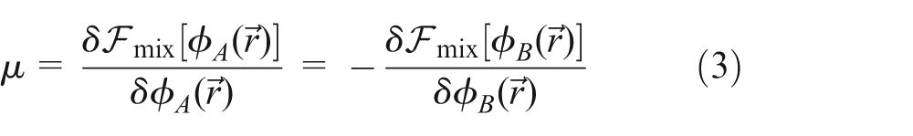
In equation (2), except for the viscoelastic stress term $\overrightarrow{\nabla }·{\mathbf{\sigma }}_{\mathrm{ve}}$ , the osmotic stress is another significant contribution originated from the thermodynamic effects. The chemical potential difference $\mu ={\mu }_A-{\mu }_B$ is defined as the functional derivative of the mixing free energy with respect to local volume fraction, that is

$$\mu =\frac{\delta {\mathcal{F}}_{\mathrm{mix}}[{\varphi }_A(\overrightarrow{r})]}{\delta {\varphi }_A(\overrightarrow{r})}=-\frac{\delta {\mathcal{F}}_{\mathrm{mix}}[{\varphi }_B(\overrightarrow{r})]}{\delta {\varphi }_B(\overrightarrow{r})}$$

(3)

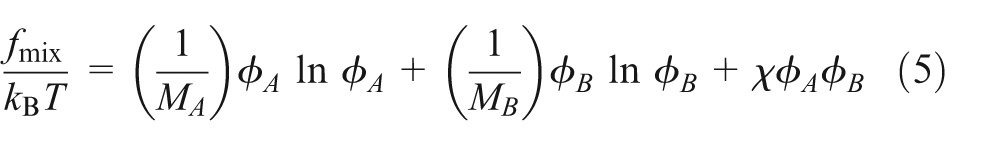
A first-order approximation of the mixing free energy functional may be given by the FH–de Gennes form as

$${\mathcal{F}}_{\mathrm{mix}}[{\varphi }_A(\overrightarrow{r})]=\int d\overrightarrow{r}\{f_{\mathrm{mix}}+\left(\frac{\Gamma }{2}\right)[\nabla {\varphi }_A{]}^2\}$$

(4)

and

$$\frac{f_{\mathrm{mix}}}{k_{\mathrm{B}}T}=\left(\frac{1}{M_A}\right){\varphi }_A\ln {\varphi }_A+\left(\frac{1}{M_B}\right){\varphi }_B\ln {\varphi }_B+\chi {\varphi }_A{\varphi }_B$$

(5)

where $\Gamma$ is the interfacial tension coefficient, $M_i$ is the molecular weight of each component polymer and $\chi$ is the FH interaction parameter.

Bringing the osmotic stress and the viscoelastic stress term together, we can get the following evolution equation for the volume fraction

$$\frac{D{\varphi }_A(\overrightarrow{r},t)}{\mathrm{Dt}}=\overrightarrow{\nabla }·[\frac{{\varphi }_A^2{\varphi }_B^2}{\varsigma }(\overrightarrow{\nabla }\mu -\alpha \overrightarrow{\nabla }·{\mathbf{\sigma }}_{\mathrm{ve}})]$$

(6)

where $\varsigma$ is a frictional coefficient and $\alpha$ is a dimensionless coefficient given by $\alpha =(1-G\prime Z\prime )/({\varphi }_A+G\prime Z\prime {\varphi }_B)$ . The chemical potential difference can be calculated from equation (3), and the total viscoelastic stress ${\mathbf{\sigma }}_{\mathrm{ve}}$ should be obtained by solving constitutive equations. Jupp and Yuan ²⁰ argued that the tube velocity should be used in the viscoelastic constitutive equation. The tube velocity may be expressed in terms of the volume average velocity by

$${\overrightarrow{v}}_{\mathrm{T}}=\overrightarrow{v}+{\varphi }_A{\varphi }_B\alpha ({\overrightarrow{v}}_A-{\overrightarrow{v}}_B)$$

(7)

and

$${\overrightarrow{v}}_A-{\overrightarrow{v}}_B=\frac{{\varphi }_A{\varphi }_B}{\varsigma }[-\overrightarrow{\nabla }\mu +\alpha \overrightarrow{\nabla }·{\mathbf{\sigma }}_{\mathrm{ve}}]$$

(8)

As equation (8) shows, the velocity difference between components A and B depends on the thermodynamic and viscoelastic forces.

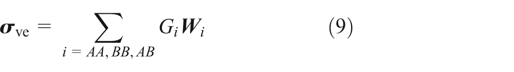
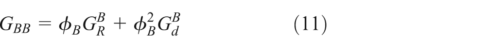
To calculate the viscoelastic forces of the mixed fluid, we split the viscoelastic stress into three parts as

$${\mathbf{\sigma }}_{\mathrm{ve}}=\sum _{i=\mathrm{AA},\mathrm{BB},\mathrm{AB}}{G}_i{\mathit{W}}_i$$

(9)

where the quantity ${\mathit{W}}_i$ is the polymer conformation tensor, whose stress $G_i{\mathit{W}}_i$ is parameterized by the elastic modulus $G_i$ . Now ${\mathbf{\sigma }}_{\mathrm{ve}}$ includes the contribution of component A, component B and an interacting part. By applying the linear rule to the Rouse process and the ‘double reputation’ rule to the disentanglement process, the elastic modulus for the three parts can be expressed as

$$G_{\mathrm{AA}}={\varphi }_A{G}_R^A+{\varphi }_A^2{G}_d^A$$

(10)

$$G_{\mathrm{BB}}={\varphi }_B{G}_R^B+{\varphi }_B^2{G}_d^B$$

(11)

and

$$G_{\mathrm{AB}}=2{\varphi }_A{\varphi }_B\sqrt{G_d^A{G}_d^B}$$

(12)

Corresponding rules for the relaxation times will be ${\tau }_d^{\mathrm{AA}}={\tau }_d^A$ , ${\tau }_d^{\mathrm{BB}}={\tau }_d^B$ and ${\tau }_d^{\mathrm{AB}}=2{\tau }_d^A{\tau }_d^B/({\tau }_d^A+{\tau }_d^B)$ . For the Rouse time, there is no interacting part, thus we have ${\tau }_R^{\mathrm{AA}}={\tau }_R^A$ , ${\tau }_R^{\mathrm{BB}}={\tau }_R^B$ and ${\tau }_R^{\mathrm{AB}}=0$ .

The RP constitutive equation for the polymer conformation tensor ${\mathit{W}}_i$ may be written as ³⁴

$$\begin{array}{cc}\multicolumn{1}{c}{\frac{D{\mathit{W}}_i}{\mathrm{Dt}}}& =2D+(\nabla {\overrightarrow{v}}_T{)}^T·{\mathit{W}}_i+{\mathit{W}}_i·(\nabla {\overrightarrow{v}}_T)\hfill \\ \multicolumn{1}{c}{}& -\frac{1}{{\tau }_d^i}{\mathit{W}}_i-f_1^i(I+{\mathit{W}}_i+f_2^i{\mathit{W}}_i)\hfill \end{array}$$

(13)

where $D=1/2(\nabla {\overrightarrow{v}}_T+(\nabla {\overrightarrow{v}}_T{)}^T)$ and the material derivative, $D{\mathit{W}}_i/\mathrm{Dt}$ , is defined in terms of the tube velocity as $(D{\mathit{W}}_i)/(\mathrm{Dt})=((\partial {\mathit{W}}_i)/(\partial t))+{\overrightarrow{v}}_T·\nabla {\mathit{W}}_i$ ; the coefficients involving the trace of the strain tensor are defined by

$$f_1^i=\frac{2}{{\tau }_R^i}(1-{(1+\frac{\mathrm{tr}({\mathit{W}}_i)}{3})}^{-\frac{1}{2}})\mathrm{for}i=\mathrm{AA},\mathrm{BB}$$

(14)

and

$$f_2^i=\beta {(1+\frac{\mathrm{tr}({\mathit{W}}_i)}{3})}^{\delta }\mathrm{for}i=\mathrm{AA},\mathrm{BB}$$

(15)

for ${\mathit{W}}_{\mathrm{AB}}$ , as ${\tau }_R^{\mathrm{AB}}\to 0$ leading to a non-stretching limit, ³¹ we obtain

$$f_1^{\mathrm{AB}}=\frac{2}{3}((\nabla {\overrightarrow{v}}_T)·\mathrm{tr}({\mathit{W}}_i+I))$$

(16)

and

$$f_2^{\mathrm{AB}}=\beta$$

(17)

In the FH–RP fluid model, $\beta$ represents the convective constraint release (CCR) magnitude coefficient and $\delta$ is a negative power specifying the exponent for the relaxation due to the CCR. For simplicity, but without much loss of generality, we assume the same value for $\beta$ and $\delta$ for the three parts of ${\mathbf{\sigma }}_{\mathrm{ve}}$ . By selecting parameter space for the FH–RP model in terms of ${\eta }_0$ , ${\tau }_R^A$ , ${\tau }_d^A$ , ${\tau }_R^B$ , ${\tau }_d^B$ , $G_R^A$ , $G_R^B$ , $G_d^A$ , $G_d^B$ ( $G_i=G_R^i+G_d^i$ ) and the shear rate, we can obtain appropriate rheology behaviour in shear flow.

Length scale, time scale and parameter sets

To study the phase behaviour under shear, we consider a system with the size of ${\Lambda }_x\times {\Lambda }_y$ , where ${\Lambda }_x=2{\Lambda }_y$ defines a rectangular simulation box. Conceptually, a shear flow of rate $\stackrel{·}{\gamma }$ can be applied by moving the upper wall boundary to the right direction at a constant speed $\stackrel{·}{\gamma }{\Lambda }_y$ . Since eliminating the finite-size effects requires a large system size, we must ensure the typical domain size $L<<{\Lambda }_{x,y}$ . Most of the recent publications^15,16,18 about the non-equilibrium phase separation tune the system size between 512 and 1024, and it is found that the finite-size effects are under control with such a system size. In this study, all simulations are done for asymmetric quenches on a ${\Lambda }_x\times {\Lambda }_y=1024\times 512$ mesh.

There exist many possible measures of the characteristic domain size. The structure factor based on Fourier transforms is usually used to define a characteristic domain size in zero-shear systems. While under shear the system is no longer periodic and the morphology will in general be anisotropic, we define the length scales using a gradient statistic for ${\varphi }_A$ across the simulation box. We define a symmetric matrix^16,18,35

$$D_{\alpha \beta }=\frac{l\int \mathrm{dx}\int \mathrm{dy}{\partial }_{\alpha }{\varphi }_A{\partial }_{\beta }{\varphi }_A}{\int \mathrm{dx}\int \mathrm{dy}{\varphi }_A^2}$$

(18)

the reciprocal eigenvalues of which give us two orthogonal length scales $L_{\parallel }$ and $L_{\perp }$ , characterizing the long and short principal axes of the domain morphology. Here, $l$ is the interface width, and it can be calculated by Helfand and Tagami’s self-consistent field theory.^36–38 Taking into account the finite chain length, Broseta et al.^39,40 predicted a broader interface and smaller interfacial tension. According to our simulation observations, Broseta’s formulation gave a more accurate description of the interfaces as

$$l=\frac{2b}{\sqrt{6[\chi -2\ln 2(\frac{1}{M_A}+\frac{1}{M_B})]}}$$

(19)

where $\chi$ is the FH interaction parameter in equation (4) and the statistical segment length $b$ may be given in terms of the interfacial tension coefficient $\Gamma$ as $b=\sqrt{18\Gamma }$ . ⁴¹ Similarly, the interfacial tension ${\sigma }_0$ may be calculated by

$${\sigma }_0=b{\rho }_0{k}_{B}T\sqrt{\frac{\chi }{6}}[1-\frac{{\pi }^2}{12\chi }(\frac{1}{M_A}+\frac{1}{M_B})]$$

(20)

where ${\rho }_0$ represents the uniform number density of monomers. The physics of binary fluid demixing can be non-dimensionalized via length scale $L_0$ and time scale $T_0$ , ¹⁶ both of which depend on the fluid density $\rho$ , the viscosity $\eta$ and the interfacial tension ${\sigma }_0$ . Here, considering the existence of viscoelastic stress ${\mathbf{\sigma }}_{\mathrm{ve}}$ , we replace $\eta$ by the total viscosity

$${\eta }_t={\eta }_0+{\eta }_p$$

(21)

thus the characteristic length and time can be given by

$$L_0=\frac{{\eta }_t^2}{\rho {\sigma }_0}$$

(22)

and

$$T_0=\frac{{\eta }_t^3}{\rho {\sigma }_0^2}$$

(23)

As described in equation (2), ${\eta }_0$ is the Newtonian viscosity contributed from the solvent or fast dynamics. The polymer zero-shear-rate viscosity ${\eta }_p$ , governed by the viscoelastic stress of the polymer mixtures, can be expressed in terms of the elastic modulus $G_i$ and the disentanglement relaxation times ${\tau }_d^i$ as

$${\eta }_p=\sum _{i=\mathrm{AA},\mathrm{BB},\mathrm{AB}}{G}_i{\tau }_d^i$$

(24)

Taking into account the mean effects of the composition field, here we assume that the polymer zero-shear-rate viscosity only depends on the initial (mean) value of ${\varphi }_A$ , thus the initial values of the composition filed ${\varphi }_A^0$ can be substituted into equations (10)–(12) to calculate ${\eta }_p$ via equation (24).

In our research on non-equilibrium steady states, the shear rate and domain size are non-dimensionalized as $\stackrel{·}{\gamma }{T}_0$ and $L_{\parallel ,\perp }/L_0$ , respectively. We consider the mesh size ${\delta }_x={\delta }_y=1$ , then in any given run, our aim is to ensure a separation of the length scales

$${\delta }_{x,y}<<l<<L_{\parallel ,\perp }<<{\Lambda }_{x,y}$$

(25)

yet we realize it is difficult to restrict the $L_{\perp }$ to significantly larger than mesh spacing with asymmetric compositions, and we will discuss this situation later in the next section.

For simplicity but without much loss of generality, we choose the following parameters: $M_A=M_B=1$ , $k_{\mathrm{B}}T=1.3$ , $\Gamma =1$ , $\varsigma =0.1$ , ${\rho }_0=1$ , $\beta =0.2$ and $\delta =-0.5$ . Thus, the equilibrium phase diagram is always symmetric with respect to ${\varphi }_A^0=0.5$ . Figure 1 shows the equilibrium phase diagram in the $\chi /{\varphi }_A^0$ parameter space of an FH fluid. $\partial f_{\mathrm{mix}}/\partial {\varphi }_A=0$ and ${\partial }^2{f}_{\mathrm{mix}}/\partial {\varphi }_A^2=0$ define the binodal and the spinodal curves, respectively. Below the binodal curve shown as a broken line in the figure, the system favours a homogeneous state in equilibrium. For $({\varphi }_A^0,\chi )$ above the spinodal (solid) line, homogeneous states are unstable and systems will spontaneously be decomposed into two coexisting phases. The critical point is at $\chi =2.0$ and ${\varphi }_A^0=0.5$ for this parameter set. Focusing on the non-equilibrium phase separation of binary polymer mixtures with asymmetric composition, we choose the $({\varphi }_A^0,\chi )$ in the two-phase region as ${\varphi }_A^0=0.3$ and $\chi =3.0$ .

Figure 1.

Equilibrium phase diagram of Flory–Huggins free energy with parameters $M_A=M_B=1.0$ and $k_{B}T=1.3$ . The homogeneous and two-phase fluid areas are bordered by binodal and spinodal lines, and between the two is a metastable region. The bold cross marks the parameters used in this article: $({\varphi }_A^0,\chi )=(0.3,3.0)$ .

As the bold cross marked in the figure shows, this point is far away from the homogeneous region at equilibrium, thus the spontaneous decomposition will take place with infinitesimal amplitude non-local fluctuations of composition. A Gaussian noise with an intensity of ${10}^{-3}$ is superimposed on the initial uniform composition field ${\varphi }_A^0$ in all simulations used for this article.

All the data sets used in our simulation runs are listed in Table 1. These runs are ordered by the values of $T_0$ . Ignoring the inertia ( $\rho =0$ ), R000 is a special case which will be used to check the role of inertia in binary viscoelastic fluids. The others could be classified into three collections with significantly different polymer zero-shear-rate viscosity ${\eta }_p$ . A large value of polymer viscosity ${\eta }_p=22.25$ is set for the cases named $R0\mathrm{xx}$ . $R3\mathrm{xx}$ and $R1\mathrm{xx}$ are allocated a smaller value, ${\eta }_p=5.5887$ and ${\eta }_p=1.2425$ , respectively. Since high shear rates give inaccuracies as described in previous publications, ¹⁶ and low values of shear rates give unacceptably long run times, we tune the shear rates in an acceptable range as $1.95\times {10}^{-3}\le \stackrel{·}{\gamma }\le 2.93\times {10}^{-2}$

Table 1.

Parameter sets used in simulations, along with $L_0$ and $T_0$ .

Name	${\eta }_0$	${\eta }_p$	$\rho$	${\sigma }_0$	$l$	$G_A$	${\tau }_d^A$	$G_B$	${\tau }_d^B$	$L_0$	$T_0$
R000	0.1	22.25	0	1.7616	7.2642	2.5	30	2.5	5.0	–	–
R001	0.1	22.25	1	1.7616	7.2642	2.5	30	2.5	5.0	283.5618	3597.642
R002	1.0	22.25	10	1.7616	7.2642	2.5	30	2.5	5.0	30.68588	404.9993
R003	0.1	22.25	100	1.7616	7.2642	2.5	30	2.5	5.0	2.835618	5.97642
R006	0.5	22.25	260	1.7616	7.2642	2.5	30	2.5	5.0	1.13001	14.59339
R005	1.0	22.25	1000	1.7616	7.2642	2.5	30	2.5	5.0	0.306859	4.049993
R007	1.0	22.25	2000	1.7616	7.2642	2.5	30	2.5	5.0	0.153429	2.024996
R301	0.05	5.5887	30	1.7616	7.2642	2.5	10	2.5	1.0	0.591013	1.875007
R302	0.05	5.5887	50	1.7616	7.2642	2.5	10	2.5	1.0	0.354608	1.125004
R303	0.05	5.5887	100	1.7616	7.2642	2.5	10	2.5	1.0	0.177304	0.562502
R304	0.05	5.5887	1000	1.7616	7.2642	2.5	10	2.5	1.0	0.01773	0.05625
R102	0.01	1.2415	10	1.7616	7.2642	0.5	10	0.5	1.0	0.087489	0.061656
R105	0.01	1.2415	50	1.7616	7.2642	0.5	10	0.5	1.0	0.017498	0.012331
R103	0.01	1.2415	100	1.7616	7.2642	0.5	10	0.5	1.0	0.008749	0.006166

Numerical results and discussions

We used a pressure implicit with splitting of operator (PISO)-based iterative solution algorithm to solve the two-fluid model. This algorithm has been well tested in a numerical study for the dynamics of polymer solutions in contraction flow. ⁴² Recently, it is adopted to study the shear-banding flows with a macroscopic two-fluid model. ³² To discretize the governing equations, we implemented the algorithms based on an Open Source computational fluid dynamics (CFD) toolbox released by the OpenCFD Ltd, named OpenFOAM. The equations are discretized through finite volume method, which locally satisfied the physical conservation laws through computing each term of the governing equations by integral over a control volume. For spatial discretization terms, the second-order Gauss MINMOD and Gauss Linear scheme are applied and the temporal terms are discretized using a simple Euler scheme. Finally, these equations will reduce to linear systems, thus using the iterative solvers predefined in OpenFOAM we can get the solutions of the equations at every time step. Typical solvers in the toolbox include the preconditioned conjugate gradient (PCG) and preconditioned biconjugate gradient (PBiCG) methods. For details, please refer to the OpenFOAM manual.

First, we will turn to the question that whether or not a non-equilibrium steady state with finite domain size exists in binary viscoelastic polymer mixtures. For all the parameter sets in Table 1 from R001 to R103, we find the domain lengths to saturate at long times with temporal fluctuations around constant mean values. Some typical runs are shown in Figure 2; both time series (except for the zero-inertia case) for $L_{\parallel }$ and $L_{\perp }$ with $\stackrel{·}{\gamma }=1.953\times {10}^{-2}$ reach a length-scale saturation in a regime that seems free of any finite-size effects. A number of additional tests are performed by changing the system size in the range of ${\Lambda }_{\parallel }=512-2048$ and ${\Lambda }_{\perp }=256-1024$ . Other tests with different shear rates between $1.95\times {10}^{-3}\mathrm{and}2.93\times {10}^{-2}$ also do not change the conclusions we report in this article.

Figure 2.

Plots of $L_{\parallel }$ and $L_{\perp }$ for various runs with $\stackrel{·}{\gamma }=1.953\times {10}^{-2}$ . Data sets for decreasing average values of $L_{\parallel }$ correspond to R000, R003, R302, R301, R303, R102 and R001. All the runs reach a steady state after $\stackrel{·}{\gamma }t=100$ , except for the zero-inertia case R000. (a) Larger domain length versus strain $\stackrel{·}{\gamma }t$ and (b) smaller domain length versus strain $\stackrel{·}{\gamma }t$ .

With $L_{\parallel ,\perp }\le {\Lambda }_{x,y}/6$ , we may conclude from these tests that the finite-size effects are fully under control. We tested several different mesh spacings with this model, which should provide us some confidences. Regarding that no any previous numerical research about the non-equilibrium steady states sets up an asymmetric composition field, we hope to give an impression with asymmetric composition field in non-equilibrium steady states.

Two typical snapshots of the steady-state composition field are presented in Figure 3 for parameter set R005. It is found that the morphologies are significantly different from the 50:50 symmetric quenches.^16,18 Although the finite-size effects appeal to be under control, the wall effects apparently get involved in our simulations. As shown in Figure 3, there are notable differences between the moving (top) wall and the static (bottom) wall. The domains near the moving wall are elongated into some short and smooth band structures, while the system favours a much smaller domain length with irregular droplets around the static wall boundary. Since our characteristic domain size $L_{\parallel ,\perp }$ only measures the average lengths across the simulation box, it cannot be concluded that such a steady state is independent of the system size. Additional tests with different system sizes support our supposition: the characteristic domain size does increase as the system size changes from $1024\times 512$ to $2048\times 1024$ . Thus, we conclude that a non-equilibrium steady state with finite domain size does exist in binary viscoelastic polymer mixtures, but the dependence of average domain size on system size cannot be strictly eliminated in our simulations.

Figure 3.

Snapshots of the steady-state composition field ${\varphi }_A$ for R005 at strain: (a) $\stackrel{·}{\gamma }t=177.71$ and (b) $\stackrel{·}{\gamma }t=234.37$ .

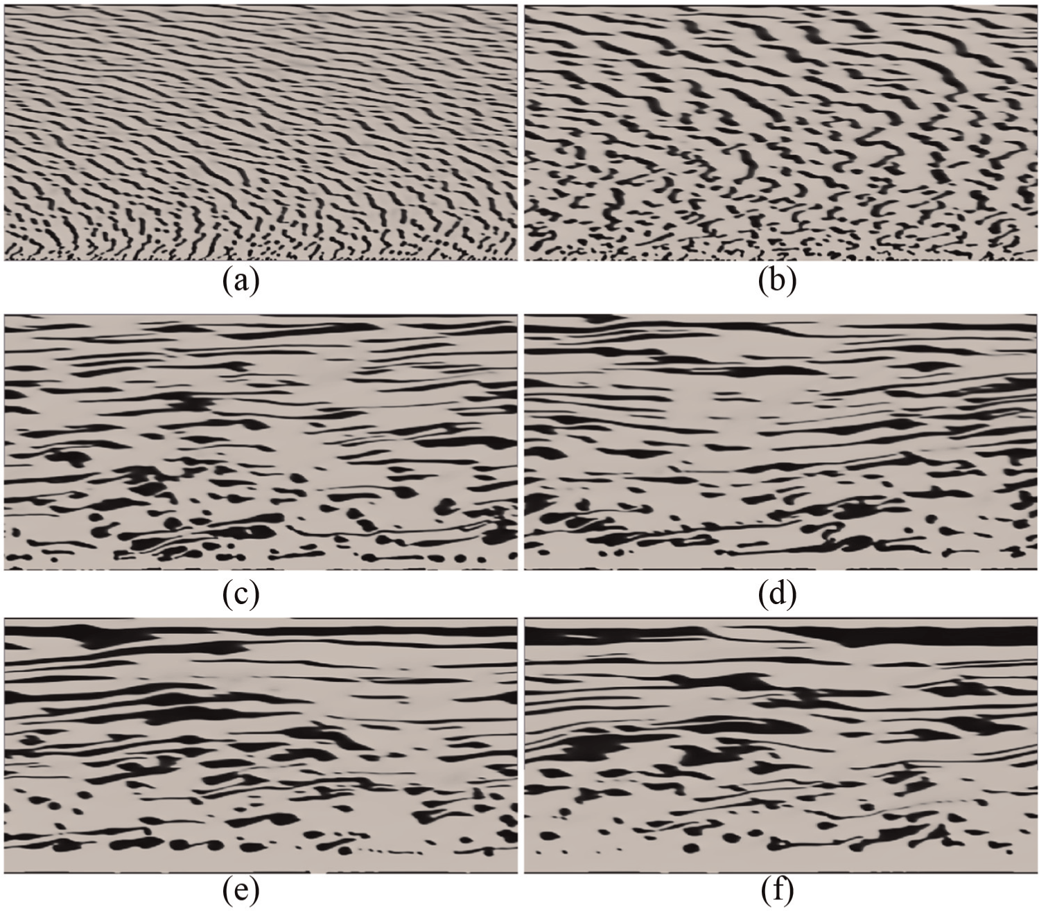
More detailed results of the phase transition from an initial homogeneous state are presented in Figure 4. At $\stackrel{·}{\gamma }t=4.85$ , the system has formed a two-phase state. The droplet patterns are rapidly stretched along the flow direction in the early diffusive regime. From $\stackrel{·}{\gamma }t=4.85$ to $\stackrel{·}{\gamma }t=9.75$ , the morphology is becoming coarser and coarser through diffusive mechanism. At late times $\stackrel{·}{\gamma }t=48.82$ and $\stackrel{·}{\gamma }t=97.3$ , the structures of composition field ${\varphi }_A$ are highly elongated, and the continuous stretching and breaking lead to slower domain growth than the diffusive regime. After a long time simulation, the system reaches a dynamical steady state similar to Figure 3. It is seen that the characteristic domain length of R001 is much smaller than R005, and wall effects still play an important role in the phase separation process. Actually, such steady states are observed in all our simulations. Phase transitions coming from visual observations for composition field ${\varphi }_A$ suggest that the length saturation stems from hydrodynamic balance between the stretching, breaking and the coalescence of domain.

Figure 4.

Snapshots of the composition field ${\varphi }_A$ at various times t for an initially homogeneous viscoelastic binary fluid. Results are obtained under applied shear rate $\stackrel{·}{\gamma }=1.992\times {10}^{-2}$ with parameter set R001: (a) $\stackrel{·}{\gamma }t=4.85$ , (b) $\stackrel{·}{\gamma }t=9.75$ , (c) $\stackrel{·}{\gamma }t=48.82$ , (d) $\stackrel{·}{\gamma }t=97.3$ , (e) $\stackrel{·}{\gamma }t=188.75$ and (f) $\stackrel{·}{\gamma }t=245.86$ .

Another important question of non-equilibrium steady state for binary viscoelastic fluids under shear is about the dependence of domain length $L$ on the shear rate. Previous research predicts a simple power law as $L~{\stackrel{·}{\gamma }}^{\alpha }$ , but the value of exponent $\alpha$ is not yet agreed upon. Some early studies^2,8 suggested a value between 1/4 and 1/3, while, even with some caution, recent numerical research^16–18 proposed the value $\alpha =3/4$ . Considering the role of viscoelasticity, the dimensionless scaling plots of steady-state length scales $L_{\parallel ,\perp }$ against shear rate are presented in Figure 5, for a series of runs in Table 1 under shear rate $\stackrel{·}{\gamma }=1.992\times {10}^{-2}$ . $L_{\parallel ,\perp }$ are obtained as the temporal means of the time series $L_{\parallel ,\perp }(t)$ , after discarding data for $\stackrel{·}{\gamma }t<100$ . It is found that (a) the data can be fitted by simple power law and apparent scaling exponents are estimated as $L_{\parallel }~{\stackrel{·}{\gamma }}^{-1.05}$ and $L_{\perp }~{\stackrel{·}{\gamma }}^{-1}$ over six decades of shear rate, with correlation coefficient $R>0.99$ ; (b) the polymer zero-shear-rate viscosity ${\eta }_p$ induces linear translation: the lines translate to the right as ${\eta }_p$ decreases. This phenomenon has not been observed in pure viscous fluids and may be attributed to the presence of viscoelastic stress.

Figure 5.

Dimensionless scaling plots of lengths versus shear rate. Error bars show the standard deviation. Solid lines: power law fits to the crosses, suggesting $L_{\parallel }~{\stackrel{·}{\gamma }}^{-1.05}$ . Dashed (red) lines: power law fits to the circles, suggesting $L_{\perp }~{\stackrel{·}{\gamma }}^{-1}$ ( $L_{\parallel }$ and $L_{\perp }$ represent two orthogonal length scales characterizing the long and short principal axes of the domain morphology, respectively). Symbols plotted from left to right correspond to the ordered data sets in Table 1.

The main distinction between our work and the previous research is that the viscoelastic effects introduced by the constitutive equations have been considered. As shown in Table 1, the viscoelastic stress is governed by the modulus $G_i$ and the disentanglement relaxation times ${\tau }_d^i$ . While the extra parameter ${\eta }_p$ can also be computed by $G_i$ and ${\tau }_d^i$ according to equation (24), changing the modulus and the relaxation times will tune both the elastic forces and the total viscosity of the fluid. Focusing on the viscoelastic effects, here we tested different parameters to generate the fluid systems with ${\eta }_p$ ranging from low $({\eta }_p=1.2415)$ to high $({\eta }_p=22.25)$ .

For the scaling exponents, the main difference between our result and previous studies of Newtonian fluids is the larger value $\alpha$ . One possible explanation may be that the total viscosity of the viscoelastic fluid in the simulations is much higher than the pure Newtonian viscosity. Since the numerical studies of zero-shear system using Boltzmann methods predict different dependencies of the characteristic domain size upon time, especially, in the viscous dominated regime $L_V~\pi t$ , which is larger than the diffusive dominated regime $L_D~t^{1/3}$ and the inertia regime $L_I~t^{2/3}$ . By substituting $t={\stackrel{·}{\gamma }}^{-1}$ in the shear-free coarsening plot, our results for binary polymer mixtures are consistent with the scaling exponents of viscous regime as $\alpha \approx 1$ .

Finally, we also test the zero-inertia systems by setting $\rho =0$ . Typical parameters are included in Table 1, named R000. From the plot of $L_{\parallel }(t)$ shown in Figure 2(a), the domain length appears to increase indefinitely as in zero-shear systems. Domain morphologies of R000 under $\stackrel{·}{\gamma }=1.992\times {10}^{-2}$ are presented in Figure 6. Initially, the scattered droplets are rapidly elongated along the flow direction; after $\stackrel{·}{\gamma }t=100$ , the domain has formed into extremely long string-like patterns, which is similar to the experimental observations under strong shear.^2,4 We also test some other parameter sets with $\rho =0$ and no evidence of non-equilibrium steady states with finite domain size is found. Our results confirm the irreplaceable role of inertia for a non-equilibrium steady state.

Figure 6.

Snapshots of the composition field ${\varphi }_A$ at various times t for an initially homogeneous viscoelastic binary fluid. Results are obtained under applied shear rate $\stackrel{·}{\gamma }=1.992\times {10}^{-2}$ with parameter set R000: (a) $\stackrel{·}{\gamma }t=19.52$ , (b) $\stackrel{·}{\gamma }t=93.74$ , (c) $\stackrel{·}{\gamma }t=152.32$ and (d) $\stackrel{·}{\gamma }t=189.44$ .

Conclusion

Non-equilibrium steady states in pure viscous binary fluid have been extensively studied, and many important conclusions are made through numerical studies with simple models ignoring the viscoelastic stress. We have numerically studied the phase separation in binary polymer mixtures with an extended two-fluid model: the FH–RP fluid model, which directly couples the thermodynamics, hydrodynamics and viscoelasticity. By solving the full equations in two dimensions, we give the first numerical study revealing non-equilibrium steady states in sheared viscoelastic fluids.

This research provides answers for some fundamental questions. First, in binary polymer mixtures, our results reveal that non-equilibrium steady states with finite domain size do exist, but the dependence of average domain size on system size cannot be strictly eliminated in our simulations. Second, we find apparent scaling exponents $L_{\parallel }~{\stackrel{·}{\gamma }}^{-1.05}$ and $L_{\perp }~{\stackrel{·}{\gamma }}^{-1}$ over six decades of shear rate. In addition, the polymer viscosity ${\eta }_p$ appears to induce linear translation of the fitted lines. It is an obvious evidence of the important role of viscoelasticity. Third, our two-dimensional (2D) simulation results show the dynamic evolution of microstructure in binary polymer mixtures with asymmetric composition under shear flow. It is found that the phase patterns are significantly different from symmetric fluids studied previously. Finally, we also identify the importance of wall effects and confirm the irreplaceable role of inertia for a non-equilibrium steady state. Apparently different domain characteristic lengths are observed near the moving wall and the static wall, which also increase the dependence of average domain size on system size in steady states. The inertia is still playing an essential role in the non-equilibrium steady states in viscoelastic polymer mixtures, since no such steady state with finite domain size is found in inertialess systems.

In future work, we aim to investigate the non-equilibrium phase separation in large-scale three-dimensional (3D) simulations. Given a more realistic free energy function, our model can accurately predict the dynamic behaviours of the systems that are not in thermal equilibrium. We will further extend this approach with the latest equations which would provide a much more realistic description of polymer free energy. We hope the realistic computational model presented here could provide valuable guidance to new experimental work and could also be used to quantitatively study some outstanding problems by appropriately selecting the parameters to mimic the real physical systems.