Sage Journals: Discover world-class research

Abstract

With the continuous consumption of fossil energy and environmental pollution, natural gas as a clean energy has received more and more attention. How to accurately predict the future of natural gas load has a vital significance. A long-term natural gas load forecasting model based on GBP is established to solve the problem of natural gas load forecasting. First, the method of correlation index is used to optimize the 20 indicators and then the optimized index number is 16; second, combining the advantages of gray neural network (BP) in fitting time series and particle swarm optimization in optimization parameters, a long-term load forecasting model of natural gas based on PSO-BP is established; finally, in order to verify the validity of the model, taking the natural gas load sample from 2005 to 2015 in Anhui Province as an example, the BP and GBP alone prediction models are compared with this model. The results show that compared with BP and GBP alone, the PSO-GBP prediction model improved the mean absolute deviation and mean absolute percentage error values by 0.065 and 0.03485 and 6.67944 and 3.62817, respectively, and increased the calculation time by 0.00726 and 0.00378 s.

Keywords

Long-term natural gas load indicator particle swarm optimization GBP BP prediction

Introduction

With the continuous consumption of fossil fuels and prominently increasing environmental pollution problems, natural gas as a clean energy has received more and more attention.^1–4 At present, China is in economic transition period, that is, changes in economic indicators have a direct impact on clean energy consumption of natural gas;^5,6 therefore, the full consideration of economic indicators has great significance on how to build an accurate long-term gas load forecasting model.

In recent years, domestic and foreign scholars have done a lot of work on the long-term load forecast of natural gas, mainly including two methods: one is the physical method,⁷ that is, the use of numerical weather forecast results, such as temperature data, and population factors, such as natural gas load curve; and the other is the statistical method, based on historical data to establish a system of nonlinear input and output mapping relationship prediction, such as genetic algorithms, dynamic gray-scale gray model, gray model, stochastic Gompertz innovation diffusion model, network model, and neuro-fuzzy-stochastic frontier model.^1,8–12 In the above statistical methods, the gray prediction method has been widely used in recent years, especially achieved good results in the small sample prediction.¹³ Since the actual prediction problem is usually uncertain and complex, and any single prediction method cannot achieve satisfactory results in different situations, that is, the single prediction method has a greater risk, the combination forecasting model has become a hot topic in the field of prediction at home and abroad.

Gray neural network combined forecasting model has achieved very good results in many fields. Based on the gray model and neural network, the gray neural network model of parallel and embedded types is proposed in Zhang and Yang.¹⁴ The thermal error of the machine tool is forecasted and good results are obtained. In Qiu et al.,¹⁵ gray neural network was used to predict the sulfur content of low-carbon ferrochromium, and the predicted hit rate reached 85%, which validated the effectiveness of the gray neural network prediction model. In Zhang et al.,¹⁶ the gray neural network model is used to forecast the container throughput of the port, and the prediction result is better than the single prediction model. In Yuan et al.,¹⁷ a gray neural network optimal combination forecasting model is established according to the characteristics of small samples and large volatility of fire accident data in China. The results show that the prediction error of this model is small and the precision is high, which is suitable for fire accident prediction. However, the gray neural network prediction model is rarely reported in the field of long-term natural gas load forecasting. Meanwhile, the gray neural network model is easy to fall into the local minimum and slow to converge,¹⁸ while the particle swarm optimization (PSO) has the characteristics of global searching and fast convergence.¹⁹ Therefore, the PSO is used to optimize the connection weights and thresholds of the gray neural network to solve the problem that the gray neural network is easy to fall into the local minimum and the convergence speed is slow, so as to improve the gray neural network prediction precision. Based on this idea, a long-term load forecasting model of natural gas based on PSO-GBP is established. In order to verify the effectiveness and the prediction accuracy of this model, the BP prediction model and the GBP prediction model alone were used for comparative analysis. The results show that the PSO-GBP long-term natural gas load forecasting model is better than BP and GBP forecasting model in both prediction accuracy and training time.

The remainder of this article is organized as follows. In section “Model theory and analysis,” model theory and analysis are described in detail; in section “Long-term natural gas load forecasting model based on PSO-GBP,” prediction steps of long-term natural gas load forecasting model based on PSO-GBP are given in detail; section “Case study” discusses a case study including selection and preprocessing of data and setting model parameter and analysis computing results; section “Conclusion” concludes the article.

Model theory and analysis

PSO theory

In the 1990s, Eberhart and Kennedy proposed a PSO algorithm²⁰ based on evolutionary computation and artificial life theory. The basic idea of the algorithm comes from the behavior of birds foraging. In PSO, each solution of the optimization problem can be regarded as a bird in the solution search space. The bird is called “particle.” Each particle is given a position and initial velocity, and the fitness function determines the fitness value of each particle; at the same time, each particle in the solution process has been given a memory function, so that in the search process, it can be very easy to remember the best location for each solution. The velocity of each particle determines the distance and direction of bird flight, so that each search is performed in the optimal solution space.

Suppose that in a $D - dimensional$ search space, population $X = (X_{1}, X_{2}, \dots, X_{n})$ is composed of $n$ particles, the population of the $i$ particle can use a $D - dimensional$ vector $X_{i} = (x_{i 1}, x_{i 2}, \dots, x_{id})^{T}$ to represent the $i$ particle in the $D - dimensional$ search space and a feasible solution to the problem. The vector $X_{i}$ is introduced into the objective function to calculate the fitness value. Then, according to the fitness value, the vector is evaluated as the optimal solution of the problem. The $i$ particle velocity is $V_{i} = (V_{i 1}, V_{i 2}, \dots, V_{id})^{T}$ , extremum is $P_{i} = (P_{i 1}, P_{i 2}, \dots, P_{id})^{T}$ . The population extreme value is $P_{gd} = (P_{i 1}, P_{i 2}, \dots, P_{id})^{T}$ . In the process of iteration, the particle updates the position and velocity through the global extremum and the individual extremum, and the updated calculation formula is given as follows

V_{id} = ω V_{id}^{k} + c_{1} r_{1} (P_{id}^{k} - X_{id}^{k}) + c_{2} r_{2} (P_{gd}^{k} - X_{id}^{k})

(1)

X_{id}^{k + 1} = X_{id}^{k} + V_{id}^{k + 1}

(2)

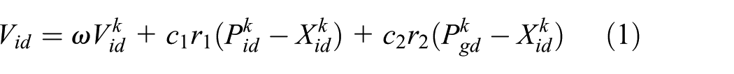
In formulas (1) and (2), $c_{1}, c_{2}$ represents the acceleration factor, which usually is a non-negative constant, and the value is [0, 1] between the random number; $ω$ represents the inertia factor; each particle keeps track of global and individual extremes in the solution space until it reaches the specified maximum number of iterations or the specified error criterion. In order to prevent each particle from being searched blindly, the velocity and position of the particle are usually limited to $[- V_{max}, V_{max}]$ and $[- X_{max}, X_{max}]$ , respectively.

As a parallel optimization and stochastic search algorithm, PSO has the advantages of good robustness, simplicity, fast convergence speed, and easy implementation. Generally, PSO can find the optimal solution of the problem with large probability. Therefore, in this article, this algorithm is used to optimize the initial parameters of GBP (gray neural network) algorithm, in order to obtain more accurate results.

GBP (gray neural network) theory

The original series of the eigenvalues of the uncertain system is $x_{t}^{(0)} (t = 0, 1, 2, \dots, N - 1)$ , and the new sequence $x_{t}^{(1)}$ is exponential growth law after one accumulation, so the data can be fitted and predicted by a continuous function or differential equation.²¹ $x_{t}^{(1)}$ is $y (t)$ , and $N$ parameters of the gray neural network model of differential equations for the expression are given as

\frac{d y_{1}}{dt} + a y_{1} = b_{1} y_{2} + b_{2} y_{3} + \dots + b_{n - 1} y_{n}

(3)

In this formula, $y_{1}$ is the output variable; $y_{i} (i = 2, 3, \dots, n)$ is the input variable; $a, b$ is the equation parameter, equation (3) solution for the expression

\begin{matrix} z (t) = (y_{1} (0) - d) e^{- at} + d = (y_{1} (0) - d) - y_{1} (0) \cdot \\ \frac{1}{1 + e^{- at}} + 2 d \cdot \frac{1}{1 + e^{- at}} \cdot (1 + e^{- at}) \end{matrix}

(4)

d = \frac{b_{1}}{a} y_{2} (t) + \frac{b_{2}}{a} y_{3} (t) + \dots + \frac{b_{n - 1}}{a} y_{n} (t)

(5)

$d$ is mapped to the extended back propagation neural network to obtain the gray neural network, the model structure shown in Figure 1.

Figure 1.

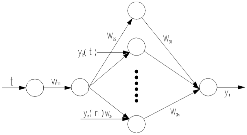
Gray neural network model structure diagram.

The weight of the input variable in Figure 1 is $ω_{11} = a$ , The weight of input layer and hidden layer is $ω_{2 i} = (2 b_{i - 1} / a)$ , $i = 2, 3, \dots, n$ . The weight of output layer and hidden layer is $ω_{3 j} = 1 + e^{- at}$ , $j = 2, 3, \dots, n$ .

Network output formula is given as follows

y_{1} = ω_{31} c_{1} + ω_{32} c_{2} + \dots + ω_{3 n} c_{n} - θ_{y_{1}}

(6)

c_{1} = h ω_{21}

(7)

c_{i} = y_{i} (t) h ω_{2 i}, i = 2, 3, \dots, n

(8)

h = \frac{1}{1 + e^{- ω_{11} t}}

(9)

θ_{y_{1}} = (1 + e^{- at}) (d - y_{1} (0))

(10)

Long-term natural gas load forecasting model based on PSO-GBP

Because PSO algorithm is easy to implement, robust, simple and has fast convergence, this article attempts to combine the PSO algorithm with GBP (gray neural network). Under the background of economic transition, based on gross domestic product (GDP) and population and other indicators, a long-term load forecasting model of natural gas based on PSO-GBP was established. First, in order to eliminate the impact on the prediction results caused by different dimensions of natural gas load and each index, natural gas load and each index are normalized, and the range is [0, 1]; second, the normalized indicators are input variables, and the natural gas load is the output variable, and BP, GBP, and PSO-GBP were used to train and forecast. Finally, the forecasting results of BP, GBP, and PSO-GBP were evaluated using mean absolute deviation (MAD) and mean absolute percentage error (MAPE), which are internationally used. The training time of BP, GBP, and PSO-GBP model are compared, and the prediction error and training time are used as the criteria to evaluate the BP, GBP, and PSO-GBP prediction models. The steps are as follows:

Step1. Selection of model input variables and output variable. The output variable should be related to the input variable;

Step 2. Because the input variables of the model have different dimensions, in order to eliminate the influence of different dimensions of the input variables on the prediction, the input variables should be normalized and the output variables should be normalized at the same time;

Step 3. According to the dimension of the input and output variables, determine the network structure of the BP and GBP;

Step 4. Initialize the particle swarm parameters, including the number of population, number of iterations, weight factor, maximum position, maximum familiarity, initial inertia weight, mutation probability, and individual upper and lower limits;

Step 5. The initial parameters of GBP were optimized by PSO, and the optimal initial GBP parameters were obtained;

Step 6. The forecasting results of BP, GBP, and PSO-GBP were evaluated using MAD and MAPE, which are commonly used in many fields.

Case study

Data selection and preprocessing

In order to verify the effectiveness of the long-term load forecasting model proposed in this article, the natural gas load statistical data of Anhui Province from 2005 to 2015 are taken as an example. As long-term load of natural gas is related to population, GDP, above-scale industrial added value, and other indicators;²² in this article, 20 objects are chosen as the input variables to influence the long-term load of natural gas and are given as follows: primary industry (billion), the secondary industry (billion), the tertiary industry (billion), the resident population (million), investment in fixed assets (million), revenue (million), government expenditure (10,000 yuan), consumer price index, commodity retail price index, industrial producer price index, industrial producer purchase price index, agricultural production price index, fixed asset investment price index, total import and export (million), the number of scientific and technological institutions (ea), scientific and technological activities (million), research and experimental development expenditure (billion), total retail sales of social consumer goods (billion), industrial enterprises above designated size, and GDP (billion) from 2005 to 2015. As the size of the input variables are different, in order to reduce the computing time and improve the accuracy of the forecast, the indicators were normalized, a specific type given in equation (11), and the normalization results are shown in Figures 2 and 3. When the BP neural network model, the forecast model selected in this article and the GBP model are used to predict, the data of natural gas load and each index from 2005 to 2013 are used as the training samples, and the data of natural gas load and each index from 2014 to 2015 as the verification sample. At the same time, the model in this article is compared with BP neural network model and GBP model separately.

Figure 2.

Normalization of year load of natural gas.

Figure 3.

Normalization of all indexes: (a) primary, secondary, and tertiary industry, (b) population, (c) investment in the fixed assets, (d) financial revenue and expenditure, (e) CPI, (f) total import and export volume, (g) science and technology agency, and (h) gross domestic product.

All of the training and simulation in this article are carried out in the MATLAB environment, using Intel^® Core™ i3-4010U 1.70 GHz processor, memory of 4.00 GB, 64-bit operating system computer platform

Y_{actual} = \frac{X_{actual} - min (X_{actual})}{max (X_{actual}) - min (X_{actual})}

(11)

Correlative analysis of year load forecasting index system of natural gas in Anhui Province

The correlation coefficient, which is an important statistical indicator measuring whether the relationship between the two variables are close and close degree, is designed by the famous statistician Pearson. The correlation coefficient is calculated according to the product moment method, which is based on the two variables and difference of the respective mean values, and the values are obtained by multiplying the two deviations to reflect the degree of correlation between the two variables. The correlation coefficient is calculated as follows

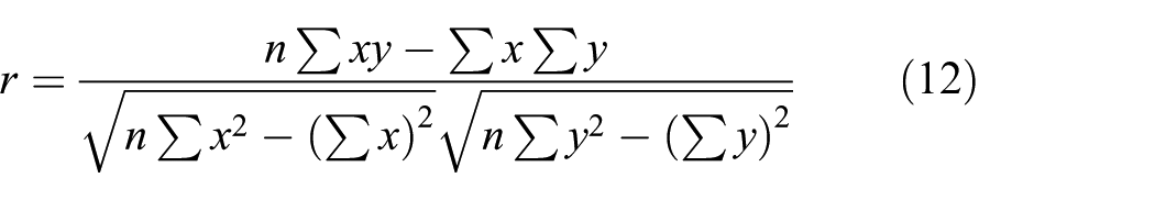
r = \frac{n \sum xy - \sum x \sum y}{\sqrt{n \sum x^{2} - {(\sum x)}^{2}} \sqrt{n \sum y^{2} - {(\sum y)}^{2}}}

(12)

In this formula, $y$ is the year load of natural gas in Anhui Province; $x$ is each index; $n$ is the amount of one index; and $r$ is correlation coefficient.

Usually, the correlation coefficient is usually between −1 and +1, that is, $- 1 \leq r \leq 1$ , and the properties of the correlation coefficients can be summarized as follows:

$r > 0$ , it means that there is a positive correlation between the two variables. $r < 0$ , it means that there is a negative correlation between the two variables.

$| r | = 1$ , it represents the relationship between the two variables is a completely linear correlation, that is, the relationship of functions.

$r = 0$ , it means that there is no linear correlation between the two variables.

$0 < | r | < 1$ , it means that there is linear correlation between the two variables; at the same time, the closer the value of $| r |$ is to 1, the closer the linear relationship between the two variables is; and the closer the value of $| r |$ is to 0, the weaker the linear relationship between the two variables is.

Generally, it can be divided into three levels: $| r | < 0.4$ indicates a low linear correlation, $0.4 \leq | r | < 0.7$ indicates significant correlation, and $0.7 \leq | r | < 1$ indicates a highly linear correlation.

The following can be calculated using formula (12): the correlation coefficients between primary industry, the secondary industry, the tertiary industry, the resident population, investment in fixed assets, revenue, government expenditure, consumer price index, commodity retail price index, industrial producer price index, industrial producer purchase price index, agricultural production price index, fixed asset investment price index, total import and export, the number of scientific and technological institutions, scientific and technological activities, research and experimental development expenditure, total retail sales of social consumer goods, industrial enterprises above designated size, and GDP in Anhui Province and natural gas are 0.99341, 0.99419, 0.98711, 0.95391, 0.99301, 0.99700, 0.99800, 0.17439, 0.03706, −0.10095, −0.20896, −0.00259, −0.00466, 0.98672, 0.94883, 0.97344, 0.9889, 0.99682, and 0.99532, respectively. The absolute value of the correlation coefficient are 0.99341, 0.99419, 0.98711, 0.95391, 0.99301, 0.99700, 0.99800, 0.17439, 0.03706, 0.10095, 0.20896, 0.00259, 0.00466, 0.98672, 0.94883, 0.97344, 0.9889, 0.99682, and 0.99532, respectively.

According to the calculation of the correlation coefficient between the indicators and natural gas load in Anhui Province, we can see: primary industry, the secondary industry, the tertiary industry, the resident population, total import and export, the number of scientific and technological institutions, scientific and technological activities, research and experimental development expenditure, total retail sales of social consumer goods, industrial enterprises above designated size, and GDP are highly linearly related to natural gas load; investment in fixed assets, revenue, government expenditure, consumer price index, commodity retail price index, industrial producer price index, industrial producer purchase price index, agricultural production price index, and fixed asset investment price index are lowly linearly related to natural gas load.

Therefore, primary industry, the secondary industry, the tertiary industry, the resident population, total import and export, the number of scientific and technological institutions, scientific and technological activities, research and experimental development expenditure, total retail sales of social consumer goods, industrial enterprises above designated size, and GDP are selected as the indexes of system year load forecast of natural gas in Anhui Province.

Setting model parameter

Since the long-term load of natural gas has a variable dimension of 16, the number of nodes in the input layer is 16; the number of nodes in the hidden layer is 17; the output layer is the natural gas long-term load; the number of output nodes is 1, namely, 16 × 17 × 1 BP nerve network structure model; the tansig function is selected as the transfer function of the hidden layer nodes; purelin function is selected as the transfer function of the output layer nodes; the maximum learning time is 19000 times; the learning speed is 0.015; and the sum of the learning object errors is 0.1.

GBP construction is based on the input and output dimensions; therefore, GBP structure is 1 × 1 × 16 × 1, the maximum learning time is 19000 times, the learning speed is 0.015, and the sum of the learning object errors is 0.1

PSO population size is set to 500, that is, 500 iterations, the two acceleration coefficient values are 1.4, the weight value of the initial value of 0.9, with the iterative progressively reduced to 0.1, the maximum velocity and position velocity are 1, the initial inertia weight is 0.9, the final inertia weight is 0.1, the mutation probability is 0.81, and the upper and lower limits of the individual range are 1 and 0.001, respectively.

Results and analysis

The collected data of the gas load from 2005 to 2015 and the indexes are normalized to get eight sets of 16-dimensional data as training samples and two sets of 16-dimensional data as test samples. Then, BP and GBP and PSO-GBP forecasting models are used, respectively, to train and test the samples. It needs to randomly generate initial parameter values a, b₁, …, b₁₅ in the gray neural network prediction. The PSO was used to optimize the 16 gray neural network initial parameters which are randomly generated at the first time. The parameters were set as given in section “Setting model parameters.” The optimization results are shown in Table 1.

Table 1.

Comparison of GBP parameter before and after PSO optimization.

Parameter	Before optimization	After optimization
a	0.8154	0.8225
b ₁	0.9950	0.8279
b ₂	0.8844	0.8341
b ₃	0.9520	0.9697
b ₄	0.9853	0.9238
b ₅	0.8262	0.8474
b ₆	0.8320	0.9238
b ₇	0.9374	0.8369
b ₈	0.9213	0.8137
b ₉	1.0226	1.0127
b ₁₀	0.9997	0.9401
b ₁₁	0.9836	1.0304
b ₁₂	0.8128	0.9742
b ₁₃	0.8128	0.9457
b ₁₄	0.8221	1.0038
b ₁₅	0.9996	1.0198

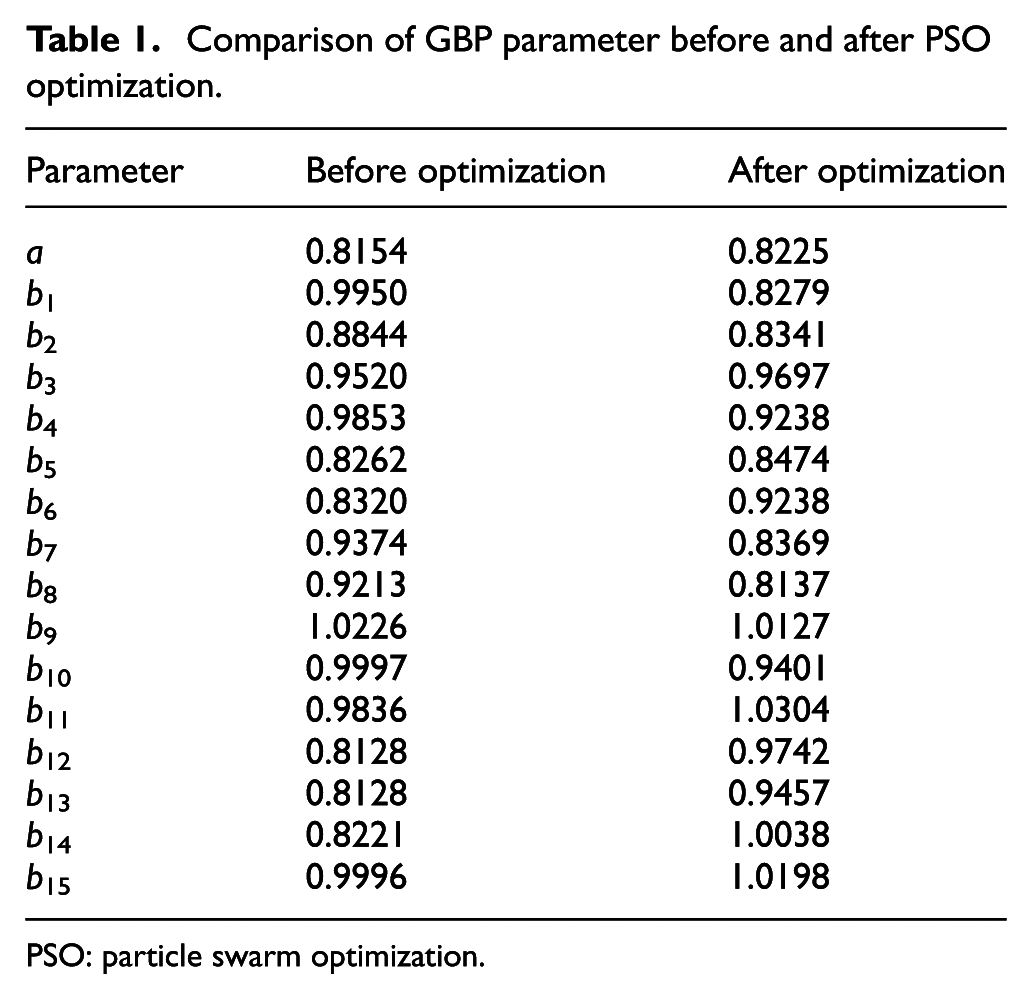
PSO: particle swarm optimization.

When comparing and analyzing different prediction models, the error evaluation standards are MAD (average absolute deviation) and MAPE (average absolute percentage error), which are common in many fields where MAD is the deviation of the predicted value from the actual value. The smaller the value is, the higher the prediction accuracy is. MAPE value less than 10 means that the prediction accuracy is high; the smaller the value is, the higher the prediction accuracy is, as shown in formulas (13) and (14)

E_{MAD} = \frac{\sum_{i = 1}^{n} | Y_{actual} - Y_{predict} |}{n}

(13)

E_{MAPE} = \frac{\sum_{i = 1}^{n} (\frac{| Y_{actual} - Y_{predict} |}{Y_{actual}})}{n} \times 100 %

(14)

In this formula, $Y_{actual}$ is the actual natural gas annual load; $Y_{predict}$ is predicted value of the BP, GBP, and PSO-GBP forecasting model; $n$ is the predicted sample number.

Figure 4 shows the comparison of training value, predicted value with the actual value of BP neural network prediction model, GBP prediction model, and PSO-GBP prediction model. It can be seen from Figure 4 that the three forecasting models can reflect the trend of the actual value. In the BP neural network prediction model, the predicted value and the actual value in 2008 and 2012 show a great deviation, and the forecast values of 2013 to 2015 are lower than the actual value; in the GBP prediction model, the predicted value and the actual value in 2014 show a great deviation, while the remaining predictions can track the change of the actual value well; in the PSO-GBP prediction model, the predicted value can track the actual value well and there is no data with larger deviation. It can be seen that PSO-GBP solves the problem well of the GBP, which is easy fall into the local minimum.

Figure 4.

Comparison of predicted values and the actual values of different prediction models.

Table 2 shows the comparison of predictive value and actual value in training time, and prediction accuracy of BP neural network prediction model, GBP prediction model, and PSO-GBP prediction model. As can be seen from Table 2, the training time of PSO-GBP prediction model comparing with BP, using GBP model alone increased by 0.00726 and 0.00378 s, and it can be seen that the initial parameters of GBP are optimized by PSO which can effectively solve the problem of slow convergence time of GBP. At the same time, the MAD value of PSO-GBP prediction model comparing with BP, using GBP model alone increased by 0.065 and 0.03485. It shows that the predicted value of the PSO-GBP model is deviated from the actual value by a smaller margin than the BP model and using GBP model alone. This is in accordance with the situation shown in Figure 4. There are no deviations of predicted values in the PSO-GBP model, and the MAPE values of the three models are all less than 8, and it indicates that all the three models have higher prediction accuracy, but the MAPE value of PSO-GBP prediction model comparing with BP, using GBP model alone increased by 6.67944 and 3.62817, and it shows that PSO-GBP prediction model has higher prediction accuracy. In summary, the PSO-GBP prediction model is superior to the BP prediction model and the GBP prediction model alone in training time and prediction accuracy and provides a new idea for the long-term load forecasting of natural gas.

Table 2.

Comparison of different prediction models.

Time and evaluation index	BP neural network	GBP	PSO-GBP	Actual value
2014	0.87417	0.88430	0.92429	0.93318
2015	0.90382	0.95399	0.98370	1.0000
Training time (s)	0.00865	0.00517	0.00139
MAPE (%)	7.97077	4.91950	1.29133
MAD	0.07760	0.04745	0.01260

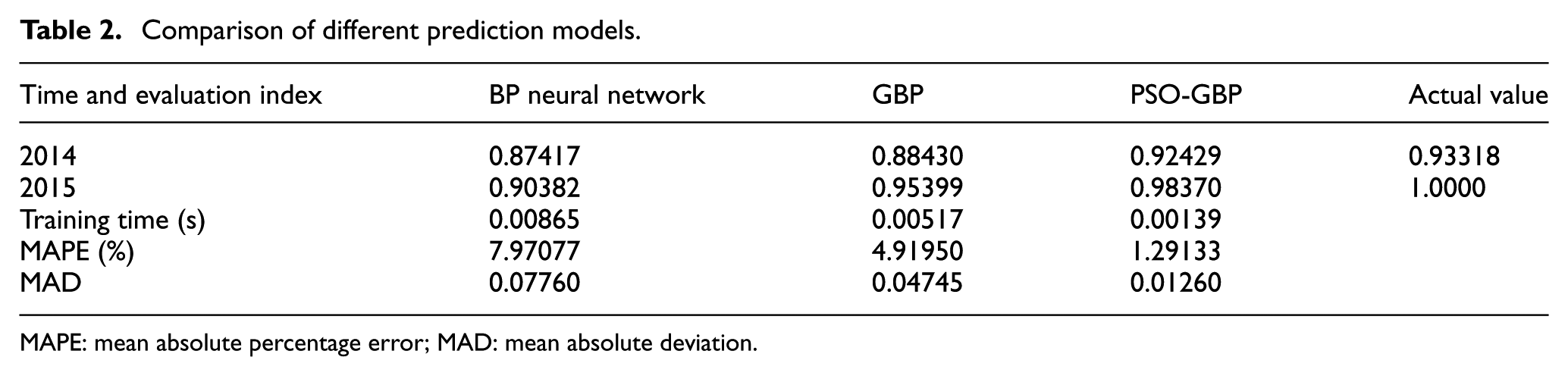
MAPE: mean absolute percentage error; MAD: mean absolute deviation.

Conclusion

Based on indicators related to long-term load of natural gas, such as GDP, above-scale industrial added value, and population, in order to solve the problem that the gray neural network is easy to fall into the local minimum and slow to converge when it is predicted, in this article, combined with the character of global search and fast convergence of PSO, a combined forecasting model of long-term natural gas load based on PSO-GBP was established. In order to verify the validity the prediction accuracy of the model, the natural gas load samples of Anhui Province from 2005 to 2015 are taken as an example and compared with the BP prediction model and the GBP prediction model separately. The conclusions are given as follows:

The method of correlation index is used to optimize the 20 indicators. The optimized indexes were primary industry, the secondary industry, the tertiary industry, the resident population, total import and export, the number of scientific and technological institutions, scientific and technological activities, research and experimental development expenditure, total retail sales of social consumer goods, industrial enterprises above designated size and GDP.

The results show that PSO-GBP combined forecasting model can solve the problem that the gray neural network is easy to fall into the local minimum and slow to converge. At the same time, PSO-GBP combined forecasting model improved the MAD and MAPE error values by 0.065 and 0.03485 and 6.67944 and 3.62817, respectively, and improved the operation time by 0.00726 and 0.00378 s compared with BP and GBP prediction model alone.

PSO-GBP combined forecasting model provides a new idea for the long-term load forecasting of natural gas.

Footnotes

Academic Editor: Jun Ren

Declaration of conflicting interests

The author(s) declared no potential conflicts of interest with respect to the research, authorship, and/or publication of this article.

Funding

The author(s) received no financial support for the research, authorship, and/or publication of this article.

References

Sánchez-Úbeda

Berzosa

. Modeling and forecasting industrial end-use natural gas consumption. Energ Econ 2007; 26: 710–742.

Reynolds

Kolodziej

. North American natural gas supply forecast: the Hubbert method including the effects of institutions. Energies 2009; 2: 269–306.

Zhang

Wood

. Sour gas reservoirs and sulfur-removal technologies: a collection of published research (2009–2015). J Nat Gas Sci Eng 2015; 26: 1485–1490.

Zhang

. Comparisons of various absorbent effects on carbon dioxide capture in membrane gas absorption (MGA) process. J Nat Gas Sci Eng 2016; 31: 589–595.

Dong

Shangguan

. Forecasting the growth of China’s natural gas consumption. Energy 2011; 36: 1380–1385.

Azadeh

Asadzadeh

Ghanbari

. An adaptive network-based fuzzy inference system for short-term natural gas demand estimation: uncertain and complex environments. Energ Policy 2010; 38: 1529–1536.

Chen

Zhang

Wei

. Analysis on temperature gradient of natural gas daily load in the winter. Nat Gas Technol Econ 2014; 8: 64–66 (in Chinese).

Nil

ARAS

. Forecasting residential consumption of natural gas using genetic algorithms. Energ Explor Exploit 2008; 26: 241–266.

Brabec

Konár

Pelikán

. A nonlinear mixed effects model for the prediction of natural gas consumption by individual customers. Int J Forecasting 2008; 24: 659–678.

10.

Gutierrez

Nafidi

Gutierrez Sanchez

. Forecasting total natural-gas consumption in Spain by using the stochastic Gompertz innovation diffusion model. Appl Energ 2005; 80: 115–124.

11.

Azadeh

Asadzadeh

Saberi

. A neuro-fuzzy-stochastic frontier analysis approach for long-term natural gas consumption forecasting and behavior analysis: the cases of Bahrain, Saudi Arabia, Syria, and UAE. Energ Econ 2007; 29: 710–742.

12.

Wang

. Forecasting China’s natural gas consumption based on a combination model. J Nat Gas Chem 2010; 19: 493–496.

13.

Zhijuan

Sun

. Prediction of air quality based on improved grey neural network model. Chine J Environ Eng 2013; 7: 3543–3547 (in Chinese).

14.

Zhang

Yang

. Grey neural network modeling for machine tool thermal error. J Shanghai Jiaotong Univ 2011; 45: 1581–1586 (in Chinese).

15.

Qiu

Zhang

Zhao

. Research on prediction model of medium-low carbon ferrochrome sulfur end-point content based on gray neural network. China Meas Test 2011; 45: 1581–1586 (in Chinese).

16.

Zhang

Xiao

. Prediction model of port container throughput based on grey neural network. J Chongqing Jiaotong Univ 2015; 34: 135–138 (in Chinese).

17.

Yuan

Song

Dong

. Study on fire accident prediction based on optimized grey neural network combination model. J Saf Sci Tech 2014; 10: 119–124 (in Chinese).

18.

Peng

. A research on natural gas load forecasting and peak shaving methods. Master graduate Dissertation, Nanjing University of Science & Technology, Nanjing, China, 2015 (in Chinese).

19.

Wang

Dong

. Prediction model of civil aviation incidents based on grey neural network. China Saf Sci J 2012; 22: 10–15 (in Chinese).

20.

Chen

Kao

. TAIEX forecasting based on fuzzy time series, particle swarm optimization techniques and support vector machines. Inform Sciences 2013; 247: 62–71.

21.

Lei

Guo

. Short-term prediction of UT1-UTC by combination of the grey model and neural networks. Adv Space Res 2017; 59: 524–531.

22.

Toksaria

. Predicting the natural gas demand based on economic indicators: case of Turkey. Energ Source Part A 2010; 32: 559–566.

Prediction of long-term gas load based on particle swarm optimization and gray neural network model

Abstract

Keywords

Introduction

Model theory and analysis

PSO theory

GBP (gray neural network) theory

Long-term natural gas load forecasting model based on PSO-GBP

Case study

Data selection and preprocessing

Correlative analysis of year load forecasting index system of natural gas in Anhui Province

Setting model parameter

Results and analysis

Conclusion

Footnotes

Declaration of conflicting interests

Funding

References