Sage Journals: Discover world-class research

Abstract

The strength and deformation of rock masses transected by persistent joints are controlled by the fracture network. In this work, bonded particle model modeled by particle flow code in three dimensions was used to study the effect of geometry parameters on the strength and behavior of jointed rock masses under uniaxial compression. The effect of the number of crossed joint sets, joint orientation, and joint spacing on the uniaxial compressive strength was investigated, and this article presents the results of the numerical simulations. Rigorous validation process had done before the numerical experiments. Four types of blocks (Series A, B, C, and D) with different numbers of joint sets were considered in this article. Then, a sensitivity study is undertaken to investigate the effects of joint set numbers and joint geometry configuration on the failure mode, unconfined compressive strength, and Young’s modulus of jointed rock mass. The interaction among the crossed joint sets was found to have marked effects on the mechanical properties and failure modes. A study about the effects of joint spacing on the failure modes, unconfined compressive strength, and Young’s modulus was also conducted. Joint spacing was found to have no significant effect on the failure modes of jointed rock masses in a certain range. It is also shown that the range and variance of unconfined compressive strength are affected principally by joint set numbers and decreased slightly with the decrease in joint spacing. The effect of crossed joint sets on the stress field was carried out. Stress concentration was found to be the reason for relatively lower strength of blocks with crossed joint sets compared to the block with the same weakest single joint set. The result in this article is of great help to reveal the mechanism of damage and fracture of jointed rocks under uniaxial compression.

Keywords

Jointed rock mass numerical analysis crossed joint sets strength analysis anisotropy

Introduction

A common problem in rock mechanics is reliable estimation of mechanical properties of jointed rock masses that consist of intact rock and discontinuities. Structure cybernetics hold that deformation and failure caused by joints played an important role in the whole rock mass engineering.^1–3 The mechanical properties of jointed rock mass, such as the compression strength and Young’s modulus, often exhibit the features of nonlinearity, anisotropy, and size effect caused by the joints. Therefore, methods that can efficiently obtain the effects of variously distributed joint sets and their interactions can be beneficial. The present methods used to describe the effect of joints on the mechanical behavior of rock mass can be classified as follows.

Analytical approaches have been taken to predict the mechanical behavior of jointed rock mass. Due to their simplifying assumptions, these methods are suited for rock mass containing regular, stratified, or orthogonal joints. The single plane of weakness theory by Jaeger and Cook⁴ is widely known, and abundant achievements^5,6 have verified the theory. In the above theory, the classical Mohr–Coulomb criterion is used to describe the failure of bedding planes, but tensile failure and interaction of the crossed joints are disregarded. The theory is extended and applied to mechanical behavior of jointed rock mass with crossed joint sets, while many laboratory experiments have confirmed the inapplicability. Although the analytical methods provide baseline solution to evaluate general approaches, the application in practical rock mass engineering is limited due to the inability to describe realistic joint systems.

The engineering classification method is an empirical technique to estimate mechanical properties of joint rock mass. Currently, many rock mass classification systems have been proposed and used in engineering practice, including the rock quality designation (RQD),⁷ the rock mass rating (RMR),⁸ tunneling quality index (Q),^9,10 geological strength index (GSI),^11,12 and rock mass index (RMi).¹³ Due to the complicated geological environment, it is difficult to construct a uniform evaluation system. The application of these empirical methods relies extensively on the engineer’s experience, especially for the qualitative description of rock and joint. Therefore, there are always some differences between the estimated and realistic properties of rock mass.

The laboratory and field testing methods are widely used; however, they suffered from the limitation caused by the rock mass anisotropy, high expense, time requirements, and complicated operation. In the laboratory tests, it is difficult to get enough jointed rock mass specimens that have the same condition due to the heterogeneity of natural rock mass. Therefore, laboratory experiments on artificial rock-like materials have been widely employed to understand the complex mechanical behavior of jointed rock mass. Numerous studies using physical modeling for a rock mass with limited joint sets^14–18 have been made. Although these studies have provided a great deal of valuable results, they generally incorporated simplifications in order to perform the tests. For example, the orthogonal joint pattern used in these physical models implies that the interaction between joint sets may be negligible. Yang et al.¹⁹ used plaster and sand to manufacture specimen containing two or three sets of non-orthogonal joints and carried out the failure mechanism and anisotropy of jointed rock mass under uniaxial compression. It is well understood that the number of joints significantly affects the stress distribution, strength, deformation, and failure of rock mass. However, few experimental studies have been performed to investigate the mechanical behavior of jointed rock mass with various configurations of joint sets.

Bonded particle model (BPM) applying particle flow code in three dimensions (PFC3D) was a step forward in numerical modeling of rock masses. In PFC3D, a rock material is simulated as an assembly of discrete rigid particles bonded together through two types of bond models: the contact bond (CB) model and the parallel-bond model.²⁰ The CB can only resist force and does not possess stiffness. The macro-stiffness is thus controlled by the particle stiffness. It implies that CB breakage may not significantly affect the macro-stiffness of the material as long as the particles remain in contact, unlikely for rock mass.²¹ The parallel bond can transmit both force and moment between particles, and the stiffness is controlled by both the contact and bond stiffness. In the parallel-bond model, bond breakage will result in a significant reduction in stiffness which may affect both the micro-stiffness of adjacent particles and the macro-stiffness of the material.²¹

Although previous experimental studies provide a general understanding of the effect of some geometrical parameters on the failure mode and strength of jointed rock mass with a single set of joint, multiple joint sets or crossed joints exist in rock mass engineering. Due to the difficulty in sampling, Kulatilake et al.^22,23 used similar material test, discrete element simulation, and particle flow code (PFC) to study the strength, deformation, and failure mode of rock mass with two crossed joint sets. In addition, a relationship between the uniaxial compressive strength (UCS) of the jointed samples of the model material and the fracture tensor component was proposed and investigated. YH Huang and SQ Yang²⁴ adopted particle flow code in two dimensions (PFC2D) to simulate the uniaxial and triaxial compression tests of jointed rock mass with two crossed joint sets, and axial tensile failure, sliding failure along joint plane, shear failure through joint plane, mixed tensile and sliding failure, and mixed sliding and shear failure are observed under uniaxial and triaxial compression. However, the weakening mechanism of crossed joints and the effect of interaction among crossed joints have not been studied comprehensively. The aim of this article is to understand the mechanisms controlling strength, deformation, stress distribution, and failure mode for multiple crossed joints. Tests of rock mass with one, two, three, and four joint sets are conducted. The analysis is divided into three stages. First, a rigorous validation study comparing PFC models to physical experiments on jointed artificial rock is undertaken. Comparisons are made on the basis of Young’s modulus, Poisson’s ratio, UCS, and failure mode under uniaxial compression. Second, the numerical model with calibrated micro-parameters is used to study the effect of joint geometrical parameters on failure mode, UCS, and Young’s modulus of a jointed rock mass. The joint geometrical parameters considered are the number of crossed joint sets, joint orientation, and joint spacing. Finally, stress field between numerical models with different number of joint sets is also compared. The relationship of cracks to axial stress is also investigated for different models with same weakest joint.

Calibration of micro-parameters and validation study

The PFC3D models blocks of rock as assemblies of spherical rigid particles with parallel bonds. Each BPM consists of 22,450 particles. The particle size, set by assigning particle radius, can be uniform or normally distributed in a given assembly. A cylinder vessel of radius 50 mm and height 100 mm was created as the boundary of the numerical model. Then, specified number of particles was generated in the cylinder vessel, and the particle radii in this numerical models presented in this article followed a normal distribution from R_min = 0.8 mm to R_max = 1.6 mm. Then, the parallel bonds are installed among all particles that are in physical contact. Flat persistent joints were created by command JSET according to design. Due to the heterogeneity and randomness of micro-strength values and the arbitrarily generated particle radius, no two PFC tests produce the same results. This feature shows a realistic simulation of natural rock material.

In the numerical experiments, the samples were loaded vertically in a constant velocity. To ensure that the specimen remained in a quasi-static equilibrium throughout the test, an adequately low loading rate was applied. A fixed loading velocity of 0.05 m/s was selected to be applied until failure occurred, which was defined as a drop in post-peak axial stress down to 80% of the peak strength. The loading velocity in the range of 0.016–0.2 m/s is used by different researchers, and selecting a lower loading velocity will result in no obvious difference for simulation results.²⁵ It is noted that “Quasi-static modeling with PFC3D usually makes usage of a high local damping coefficient to efficiently remove kinetic energy from the system. Therefore typical quasi-static deformation can be performed at a much higher rate than in real experiments.” (Emam S, 2013, personal communication). The laboratory uniaxial compression test adopted a loading rate of 0.5–0.8 MPa/s stress-control loading. Figure 1 shows the jointed model with two crossed joint sets; the particles crossed by joints are shown in black and dark gray to distinguish from the other particles.

Figure 1.

Numerical model of jointed sample with two sets of crossed joints.

In this section, the ability of BPM to reproduce actual values of UCS, Young’s modulus, and failure mode of jointed rock masses with multiple crossed joint sets recorded in laboratory experiments are explored.

The micro-parameters of the BPM and joint have to be calibrated prior to the numerical analysis. In order to calibrate the BPM micro-parameters, numerical uniaxial and triaxial compression tests on cylindrical samples are undertaken and the micro-parameters are determined by trial and error to reproduce the macro-scale properties measured in physical experiments. For the calibration of joint parameters, numerical direct shear tests and normal deformation tests are carried out and also calibrated against those physical experiments.

After calibration of the micro-parameters, four series of numerical models for jointed rock mass with different numbers of joint sets are generated, and uniaxial compression tests are undertaken.

Calibration of particle parameters

In order to calibrate BPM micro-parameters, cylindrical samples with diameter of 50 mm and height of 100 mm are generated. Inverse modeling is employed to calibrate micro-mechanical properties of BPM against experimental uniaxial and triaxial compression tests in laboratory. Calibration involves selection of the micro-properties by an iterative process to reproduce the mechanical properties of intact rock on the laboratory scale. The first step of iteration is calibration of Young’s modulus (E). Particle contact modulus (E_c), particle normal/shear stiffness ratio (k_n/k_s), parallel-bond modulus $({\bar{E}}_{c})$ , and parallel-bond normal/shear stiffness ratio ( ${\bar{k}}_{n} / {\bar{k}}_{s}$ ) are micro-parameters influencing E. The second step is matching Poisson’s ratio (v) controlled by k_n/k_s and ${\bar{k}}_{n} / {\bar{k}}_{s}$ . This is followed by calibration of the UCS σ_ci influenced by normal strength and shear strength of parallel bonds. Finally, the coefficient of friction µ is calibrated applying the results of triaxial compression tests. The calibrated micro-properties of particles and parallel bonds are summarized in Table 1. Results of the uniaxial and triaxial compression tests on the calibrated BPM model are compared with the experimental results in Table 2. Results of the calibrated numerical model tests correspond well with those of experimental tests.

Table 1.

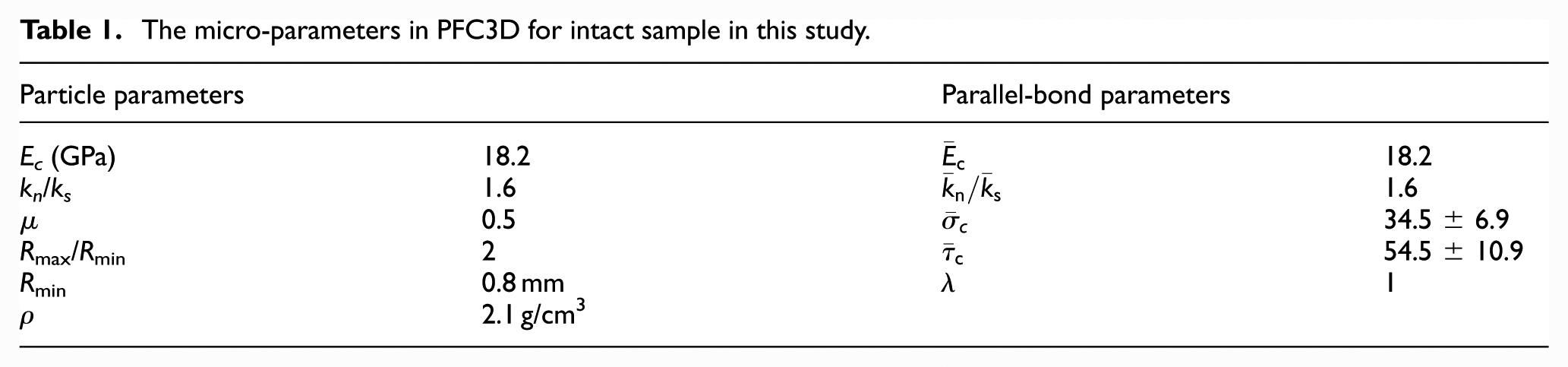
The micro-parameters in PFC3D for intact sample in this study.

Particle parameters		Parallel-bond parameters
E_c (GPa)	18.2	${\bar{E}}_{c}$	18.2
k_n/k_s	1.6	${\bar{k}}_{n} / {\bar{k}}_{s}$	1.6
µ	0.5	${\bar{σ}}_{c}$	34.5 ± 6.9
R _max/R_min	2	${\bar{τ}}_{c}$	54.5 ± 10.9
R _min	0.8 mm	λ	1
ρ	2.1 g/cm³

Table 2.

Comparison of material properties of physical experiment and numerical study.

Macro-properties	Physical experiment	BPM
Uniaxial compressive strength (UCS, MPa)	47.01	46.82
Young’s modulus (E, GPa)	20.2	20.4
Poisson’s ratio	0.2	0.205
Specimen size (mm)	54/108	50/100

BPM: bonded particle model.

Calibration of joint parameters

The micro-parameters of joint sets are normal stiffness ${\bar{k}}_{nj}$ , shear stiffness ${\bar{k}}_{s j}$ , normal parallel-bond strength ${\bar{σ}}_{nj}$ , shear parallel-bond strength ${\bar{σ}}_{sj}$ , and coefficient of friction µ_j. To determine these parameters, laboratory direct shear tests and normal deformation tests are conducted on samples of model material with smooth horizontal joints to determine the shear strength behavior and normal deformation of the model joints. Epoxy resin adhesive is employed to glue the rock blocks as the joint sets.

Numerical samples of diameter 50 mm and height 50 mm are generated. The flat joints in the numerical model are simulated by reducing the micro-mechanical parameters of the parallel bonds along the location of joints. In order to calibrate ${\bar{k}}_{nj}$ , normal deformation tests are carried out. In addition, for calibration of ${\bar{k}}_{s j}$ , ${\bar{σ}}_{nj}$ , ${\bar{σ}}_{sj}$ , and $μ_{j}$ , direct shear tests are undertaken.

In the numerical normal stiffness test, after generation of the sample, lateral restraints are removed and a horizontal joint plane is inserted at mid height of the sample by the command JSET. Normal stress is applied to the upper surface, and the stress and the vertical displacements are recorded during the loading process until the normal stress reaches one-third of the UCS of the intact material. The inverse calibration method is used to determine ${\bar{k}}_{nj}$ . It means that ${\bar{k}}_{nj}$ will be varied until macro-normal stiffness on the laboratory scale is achieved.

In the numerical direct shear test, a constant normal load is applied vertically to the upper block and a servo control mechanism is used to keep the normal load constant during the shearing process.²⁶ The lower block is kept stationary during the test and a horizontal velocity of 0.005 m/s is applied to the upper block. In PFC, calculations are based on an explicit time-stepping algorithm. A three-stage inverse modeling procedure is applied to calibrate the other joint parameters. First, planar joint shear stiffness ${\bar{k}}_{s j}$ is varied to reproduce the system shear stiffness on the laboratory scale (K_s = 4.9 GPa/m), and normal stiffness ${\bar{k}}_{nj}$ is varied to achieve the normal stiffness on the laboratory scale. Second, the smooth joint coefficient of friction $μ_{j}$ is varied to achieve the laboratory-scale coefficient of friction. Third, the shear parallel-bond strength ${\bar{σ}}_{sj}$ and normal parallel-bond strength ${\bar{σ}}_{nj}$ are varied to achieve the shearing strength on the laboratory scale. The calibrated macroscopic properties of the joints determined from the numerical result with calibrated micro-parameters and laboratory tests are summarized in Table 3. The test results of the calibrated model are in good agreement with those of the laboratory experiments.

Table 3.

Macro-mechanical parameters of the joint and the attenuate coefficient of parallel-bond mechanical parameters along the joint.

Test results
Macro-mechanical parameters	Experiments	Numerical
Normal stiffness (GPa)	19.80	19.72
Shear stiffness (GPa)	4.90	4.85
Cohesion (MPa)	3.22	3.25
Frictional coefficient	0.74	0.752
Parallel-bond mechanical parameters on the joint
Parallel-bond normal strength (MPa)	3.45
Parallel-bond shear strength (MPa)	5.45
Parallel-bond normal stiffness (GPa)	7580
Parallel-bond shear stiffness (GPa)	4740
Frictional coefficient	0.05

Simulation of jointed rock mass and comparison with physical experiments

The jointed rock mass modeled in this article is brittle rock with cement faces, and the thickness of the joint set is ignored. Laboratory testing on a rock mass containing a specified number of joints with predetermined orientations is nearly impossible. One common method to solve the problem is to select a modeling material for brittle rocks. Two characteristics of the material are considered here to ensure the suitability of modeling material: (1) brittle character of the modeling material and (2) dilatancy of the material under uniaxial compression.

The rock-like material used in preparing the intact samples was a mixture of plaster, sand, and water in the following proportion by weight: (a) river sand (dry, diameter less than 1 mm), 58%; (b) Portland cement, 29%; and (c) water, 13%. To ensure the maximum possible homogeneity and isotropy of the overall compound, the river sand and Portland cement were initially mixed together prior to the addition of water. Subsequently, water at room temperature was added to the dry mix of the constituents and thoroughly re-mixed. The mixed material contained a lot of air. So, the mixed material was put in the wooden mold by three steps, and the shaking table was used to eliminate the air adequately at every step. For jointed samples, steel slices are inserted into the homogeneous mixed material according to the experiment design and removed 12 h later. Each primary sample was kept in water with temperature controlled at 25° ± 2° for 28 days. Then, the dry jointed samples were glued by epoxy resin adhesive and kept standing for 2 days. Finally, core-drilling machine and cutting machine were employed to make cylindrical samples of 54 mm diameter and 108 mm height. It should be noted that the consistency of mixing, curing, and testing is required to obtain reproducible test results.

After calibration of the BPM and joint micro-parameters, the cylindrical numerical samples identical to physical samples in laboratory are generated. Four series of A–D samples with different joint set numbers are considered, and various subseries for different joint configurations are considered (Table 4). For every series (A–D), no joint sets with the same dip angle exist among the subseries. Two kinds of joint spacing (10 and 20 mm) are also considered for every subseries. Subscript 10 and 20 representing the sample joint spacing is 10 and 20 mm, respectively, such as A1₁₀. Three parallel joints are set for every set of joint to eliminate the effect of joint number, and the concentrate joints are the main structure which affects the behavior of rock samples.

Table 4.

Subseries and corresponding joint configurations.

Subseries	A1	A2	A3	A4	A5	A6	A7	B1
Dip angles (°)	0	15	30	45	60	75	90	0, 90
Subseries	B2	B3	B4	C1	C2	C3	D1	D2
Dip angles (°)	15, 75	30, 60	45, 45	0, 60	15, 75, 45	30, 90	0, 45, 90	15, 45, 60, 75

After generation of all the 16 subseries of BPM, numerical uniaxial compression tests are carried out and results are compared with the laboratory experiments of artificial synthetic material. Results of partial subseries for physical and numerical studies are presented in Table 5. Three typical failure modes of tensile split, slide failure, and mixed failure are observed in both the numerical and experiments tests shown in Table 6. Comparison between the numerical and experimentally determined failure mode verified the ability of PFC model to reproduce failure mode of a jointed rock mass with multiple crossed joints.

Table 5.

Results of physical and numerical tests.

Subseries	A1		A3		B3		B4
Properties	UCS (MPa)	E (GPa)	UCS (MPa)	E (GPa)	UCS (MPa)	E (GPa)	UCS (MPa)	E (GPa)
Physical test	39.05	19.88	35.16	18.76	14.13	17.24	19.57	16.79
Numerical test	40.99	19.67	34.93	19.31	13.54	16.76	20.13	17.41

Table 6.

Typical failure modes of physical and numerical tests.

Subseries	A1	A3	B3	B4
Physical test
Numerical test

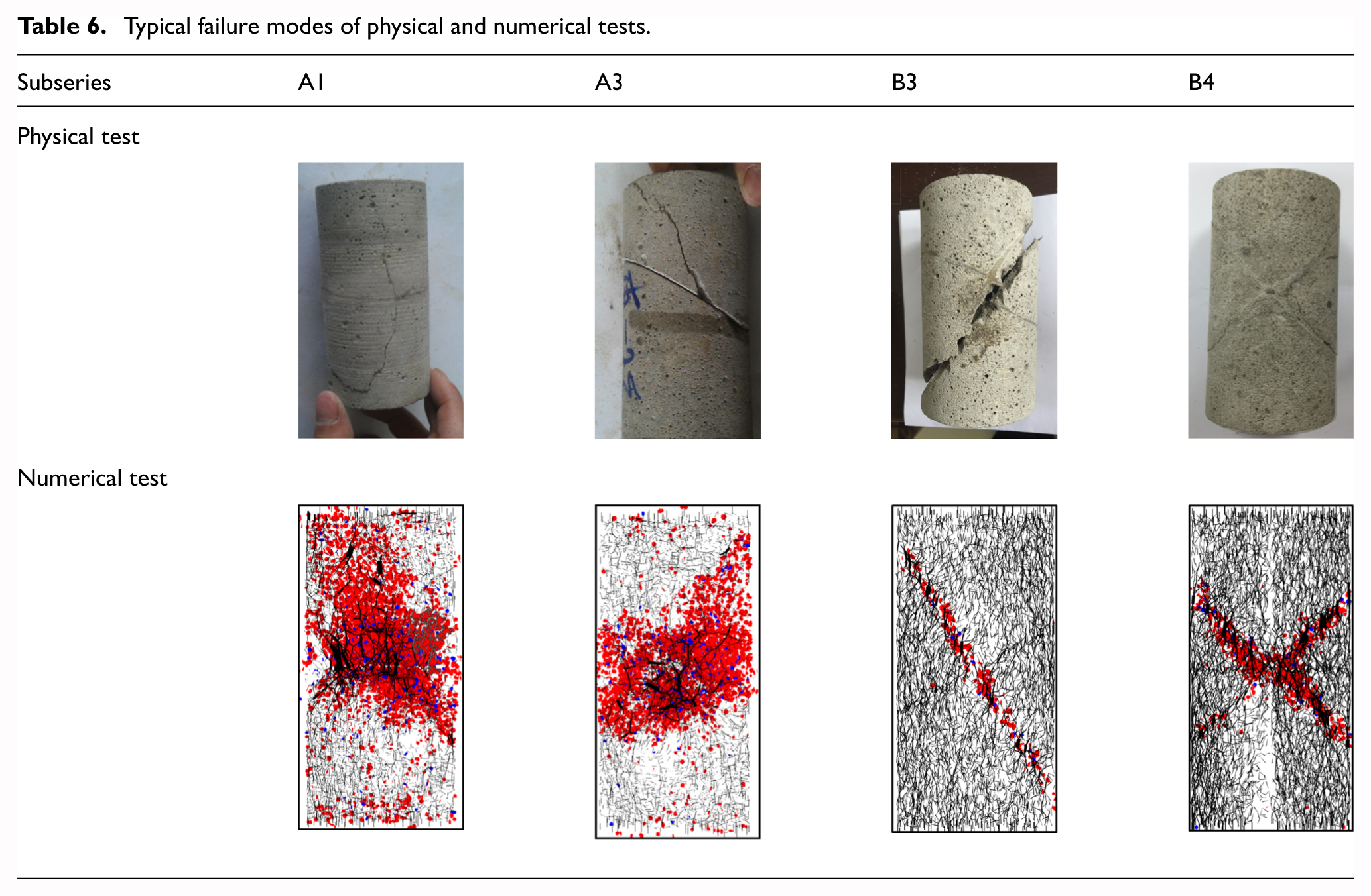
Table 6 displays the comparison of failure modes between the results of laboratory physical tests and numerical simulations for rock samples A1, A3, B3, and B4. For Subseries A1, the jointed synthetic rock block in the physical experiment mainly failed through intact block, and the direction of initial failure is parallel to the loading direction. The corresponding numerical model also shows an axial failure path through the intact block.

For Subseries A3, the main failure mode involves tensile failure of intact block and joint slide. Macro-fracture can be seen in the precast joint and the intact material. The numerical model for A3 shows a main failure path being similar to that of the physical experiment sample.

For Subseries B3, sliding occurred along the joint plane, and the main failure path is clearly along the joint surface with joint dip angle 60°. There is always a weak joint occurring in the jointed rock mass which fails along a joint surface. The corresponding numerical model shows a same failure mode through the joint surface.

For Subseries B4, X-shaped fracture formed by two failure planes can be seen on the physical experimental samples. It is a particular situation for the above failure mode. There are two weak joints occurred in the block, and the two joints have the same dip angle and opposite dip directions. The jointed rock mass is separated into multiple blocks along the joints under uniaxial compression. The aforementioned comparison shows that the calibrated numerical model possesses the capability to reproduce the failure modes. It can be seen on the blocks used for physical experiments. It is implied that the calibrated numerical model had the capability to produce accurate values for jointed block strength and proper failure modes for jointed rock masses.

Effect of joint sets number on the mechanical properties of a jointed rock mass

In order to find the influence of each geometrical parameter on the failure mode, UCS, and Young’s modulus E, a sensitivity study was undertaken using the BPM approach. Uniaxial compression tests were carried out on numerical models with various joint configurations. The parameters considered are the joint orientation and the number of joint sets.

Four types of blocks with different numbers of joint sets are generated in this article to investigate the effect of joint sets number on the mechanical properties and failure mode. Block A represents the block with one set of joint, and the dip angles of joints are varied from 0° (horizontal, A1) to 90° (vertical, A7) with an increment of 15°. Block B represents the block with two orthogonal joints, and B1 (0° and 90°), B2 (15° and 75°), B3 (30° and 60°), and B4 (45° and 45°) are generated. Block C represents the block with three crossed joints, and the angle between adjacent joints is equal to 60°. So, C1 (0° and 60°), C2 (15°, 75°, and 45°), and C3 (30° and 90°) are generated. Block D represents the block with four crossed joints, and the angle between adjacent joints is equal to 45°. D1 (0°, 45°, and 90°) and D2 (15°, 30°, 60°, and 75°) are generated for Block D.

UCS

Using the above calibrated parameters, simulations are performed for four types of blocks. In this article, the distribution of the joint sets is symmetrical, and the angles between the adjacent joint sets are equal. Blocks A, B, C, and D represent the number of joint sets, respectively: one joint set, two orthogonal joint sets, three crossed joint sets, and four crossed joint sets. Figure 2 shows comparison of strength of the ratio UCS_j/UCS_i between numerical and physical tests for block with the different number of joint sets and different combinations of joint dip angles. UCS_j and UCS_i are the unconfined compression strength of jointed model and intact model, respectively. The results of laboratory tests in Figure 2 are average values of the unconfined compressive strength of three same samples. We can observe from Figure 2 that the results of numerical tests are consistent with the experimental data. The maximum strength difference between the numerical and physical test results is less than 5%.

Figure 2.

Comparison of the strength ratio UCS_j/UCS_i between numerical and physical tests for different subseries of blocks.

From Figure 2, the following results are obtained:

1. For Series A, the orientation of joint has a significant effect on the UCS of model. The UCS is considerably high for joint dip angle β close to 90° or in the range of 0°–30°, compared to the case for joint dip angle β in the range of 40°–80°. The UCS_j/UCS_i is found to be the lowest for β in the range of 60°–75°. The variation range of UCS_j/UCS_i is approximately from 0.25 to 0.87.

It should be noticed that the UCS_j changes with the variation in joint strike-angle when the dip angle is constant. The reason for the variability of strength is the distribution of the particles, and the range of ${UCS}_{j}^{r} / {UCS}_{j}^{av}$ ( ${UCS}_{j}^{r}$ and ${UCS}_{j}^{av}$ are the uniaxial strength of the single joint model with a random strike-angle and average uniaxial strength of the single joint model with random strike-angles, respectively) is less than 5%. So, the variability of the strength is ignored in this article.

2. With the increase in the number of crossed joints, the effect of joint orientation on UCS_j/UCS_i gradually diminishes. However, the UCS_j/UCS_i variation with β shows the wave-like shape because of the symmetry of the crossed joints. For Series B, the variation in UCS_j/UCS_i is approximately from 0.25 to 0.77. For Series C, the variation in UCS_j/UCS_i is approximately from 0.25 to 0.48. In addition, for Series D, the effect of the joint orientation on the UCS_j/UCS_i diminishes ulteriorly. The variation in UCS_j/UCS_i is approximately from 0.23 to 0.36. It is clear that the maximum of UCS_j/UCS_i decreased sharply with the increase in joint sets, while the minimum varied slightly.

3. The UCS of block with multiple crossed joints is significantly lower than Series A except for the model with joint dip angle 60° or 75°. The UCS of the jointed model is dominated by the weakest dip angle, so the UCS of model does not decrease with the increase in crossed joint sets strictly. For the models with joint dip angle 60° or 75°, the strength of model with two crossed joints is similar to the model with single joint because the dip angle of the dominated joint is 60° or 75°, and the strength of model decreases slightly with the increase in the number of joint sets.

4. It is noteworthy that the effect of the interaction between the crossed joints on the UCS of model is also obvious. For example, the UCS of B4 (dip angles 45° and 45°) is apparently lower than the UCS of A4 (dip angle 45°) though the dip angles of weakest joints are both 45°. In addition, the UCS of C1 (dip angles 60°, 60°, and 0°) is slightly lower than the UCS of the model with one or two joints, though their weakest dip angles are both 60°.

The anisotropy of UCS is represented by the range and variance of UCS for different types of blocks as Table 7 shows. It is clear that the range and variance of UCS decrease obviously with the increase in joint sets.

Table 7.

The range and variance of UCS for different series.

	A	B	C	D
Range	0.623	0.521	0.238	0.135
Variance	0.270	0.237	0.116	0.072

Stress–strain response

Figure 3 shows the stress–strain curves during compression for the different types of models at zero confinement. As shown in Figure 3, the axial strain at peak strength is discrete and varies sharply with dip angles. The range of axial deformation decreases with the increase in joint sets. Actually, the minimum axial deformation of the four series of models is similar (nearly 8e−4), while the maximum axial deformation decreases with the increase in joint sets. The variability of peak strength is similar to axial strain at peak strength.

Figure 3.

Stress–strain curve under uniaxial compression for (a) Series A, (b) Series B, (c) Series C, and (d) Series D.

The initial post-peak response is brittle for blocks with high uniaxial strength, but the ductility increases for the model with low uniaxial strength. The initial post-peak response becomes obviously ductile for A6, B2, and C2. This is because the dip angle of weakest joint sets in the above blocks is 75°. The uniaxial strength remains in the post-peak phase because the joint set with 75° angle crossed the top and bottom of the block.

Figure 4 shows the influence of joint sets number on Young’s modulus under uniaxial compression. Young’s modulus of the model decreases with the overall increase in joint sets. Young’s modulus is independent of dip angle for Series A, except for Subseries A5 and A6. In this case, deformation along the joint contributes majority of the axial deformation. Young’s modulus is sensitive to the number of crossed joint sets as Figure 4 shows. The effect of joint sets on Young’s modulus for the other series is likely to be the simple addition of all existing joint sets.

Figure 4.

Young’s modulus of Series A, B, C, and D under uniaxial compression.

Failure modes

Table 8 shows the failure modes of the synthetic jointed samples with different numbers of joint sets. Contact force between contiguous particles in the range of x (−0.01, 0.01) and all cracks in the whole model appearing at a certain stress state along the axial direction are displayed in the cross-sectional surface. For each case, an image displays the bond breakage level when the stress drops to 0.8σ_p in the post-peak phase. Red disk and blue disk represent the tensile cracks and shearing cracks, respectively. Orientation and thickness of the black segment represent the direction and magnitude of the contact force, respectively, in Table 8.

Table 8.

Effect of number of joint sets on the failure modes.

A1	A2	A3	A4	A5	A6	A7	B1

B2	B3	B4	C1	C2	C3	D1	D2

Subseries A1, A2, A7, and B1 failed in tensile splitting. In this mode, bond breakages begin to appear at the joint surface when the model is loaded in the axial direction. Then, bond breakages occur evenly around the joint and extend along the axial direction, a macro failure plane is formed at peak stress.

The failure mode of Subseries A4, A5, A6, B2, B3, and C2 was planar. In this mode, bond breakages occur along the joint surface at the beginning, and the stress concentrates along the joint face. Shearing and tensile failure occur through the pre-existing joint sets, and then, a macro planar failure plane appears at the peak stress. The distribution of bond breakages is obviously narrower than the other failure modes. It should be noticed that the bond breakage and stress concentrate around the crossing point of top surface and joint set with dip angle 75°.

Subseries B4, C1, C3, D1, and D2 failed under X-shaped failure mode. It is a particular situation of the above failure mode. In this mode, multiple crossed joint sets occur in the model, and planar failure occurs in two of them. Then, the model is cut into small pieces of blocks, and two crossed failure planes appear at the peak stress as Table 8 shows.

Subseries A3 failed in mixed mode of tensile splitting and planar failure, and both of the tensile splitting in intact rock and the planar failure along the pre-existing joint sets occurred in this failure mode. The dip angle in main joint set is 30°–40°, which is close to 45°–θ/2. The bond breakages occur around the joint set at the beginning and extend to the intact block with the increase in stress. The failure path consists of the intact failure and joint slide at the peak stress.

It should be noted that Subseries B4, C1, C3, D1, and D2 could also fail under planar failure mode in physical uniaxial tests as Figure 5 shows. Both planar and X-shaped failure may happen. Unlike the idealized numerical models, the strengths of symmetrical joints are impossible to be the same absolutely, because the thicknesses and uniformity of the artificial joints have some difference due to the effect of artificial manufacturing. With the increase in axial load, micro-cracks generated and formed a macro-fracture along the weaker joint, while the other joint was seemingly faultless. This could result in the planar failure instead of X-shaped failure for the above-mentioned blocks.

Figure 5.

Planar failure mode of physical sample B4, C1, C3, D1, and D2.

Effect of joint spacing on the mechanical properties of a jointed rock mass

UCS

The joint spacing is also a significant factor for the strength and deformation properties of a jointed rock mass. The effect of joint spacing D is investigated by taking joint spacing D = 10 and 20mm and the joint set number is also variable.

The effect of joint spacing on the uniaxial strength and failure mode is shown in Figure 6. The model with single joint for every joint set represents the model with joint spacing which is much larger than 20 mm. Joint spacing D = 10 and 20 mm is taken to investigate the effect of joint spacing on the uniaxial strength. Subscripts 10 and 20 mean the model with joint spacing 10 and 20 mm, respectively.

Figure 6.

Effect of joint spacing on the uniaxial strength for A, B, C and D models.

For all types of models with joint spacing 20 and 10 mm, the uniaxial strength of them decreases obviously, compared with the block with single joint for every joint set. For Series A (block with one set of joint), effect of joint spacing varies with the joint orientations. The uniaxial strength of A1, A2, and A7 is positively related to the joint spacing, while the uniaxial strength of A3, A4, A5, and A6 remains substantially unchanged with varying joint spacing.

For Series B (block with two sets of joint), effect of joint spacing varies with the combination of joint dips. The uniaxial strength of B1 (β = 0°, 90°) and B2 (β = 15°, 75°) increases significantly with the increase in joint spacing, while the uniaxial strength of B3 (β = 30° and 60°) and B4 (β = 45°) remains substantially unchanged with varying joint spacing.

For Series C (block with three sets of joint), effect of joint spacing on the uniaxial strength is significant except for C2 (β = 15°, 45°, and 75°).

For Series D (block with four sets of joint), effect of joint spacing on the uniaxial strength is significant for all the cases. In addition, the strength reduction is insensitive to the joint dips.

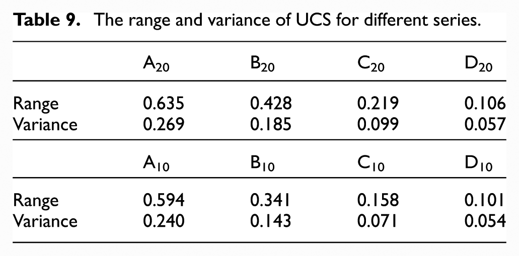
The anisotropy of UCS is represented by the range and variance of UCS for different types of blocks as Table 9 shows. It is clear that the range and variance of UCS decrease obviously with the increase in joint sets, and they decrease slightly with the decrease in joint spacing.

Table 9.

The range and variance of UCS for different series.

	A₂₀	B₂₀	C₂₀	D₂₀
Range	0.635	0.428	0.219	0.106
Variance	0.269	0.185	0.099	0.057
	A₁₀	B₁₀	C₁₀	D₁₀
Range	0.594	0.341	0.158	0.101
Variance	0.240	0.143	0.071	0.054

Stress–strain response

Figure 7 shows the stress–strain curve of model with different numbers and different joint spacing of joint sets during uniaxial compression. The stress–strain curve is marked as solid symbol for joint spacing D = 10 mm and hollow symbol for joint spacing D = 20 mm for the corresponding blocks. The stress–strain curve shape is similar for the same kinds of blocks with different joint spacing.

Figure 7.

Stress–strain curve under uniaxial compression for: (a) Series A_10,20, (b) Series B_10,20, (c) Series C_10,20, and(d) Series D_10,20.

The axial deformation at peak strength for blocks with joint spacing 10 or 20 mm is discrete and the variations are similar to the model with single joint for every joint set. The effect of joint spacing on the axial deformations at peak strength is unapparent except for Subseries A1, A2, A7, B1, and C3.

Figure 8 shows the influence of joint spacing on Young’s modulus of rock mass under uniaxial compression. In theory, joint spacing has no effect on Young’s modulus for the same joint number, but Young’s modulus of A5₁₀, A6₁₀, and A7₁₀ is lower than A5₂₀, A6₂₀, and A7₂₀, respectively. This is due to the model size and arrangement of joints. The joint surfaces in Subseries A5 and A6 cross top or bottom of the blocks, and then, the axial component of joint deformation decreases. For Subseries A7₂₀, two joint surfaces do not work because they are placed on the edge of the block. In the same way, Young’s modulus decreases with the decrease in the joint spacing for all the blocks except for Subseries B4, as shown in Figure 8. Actually, Young’s modulus is sensitive to the joint spacing for the rock mass with large enough size because the number of joints increases with the decrease in joint spacing.

Figure 8.

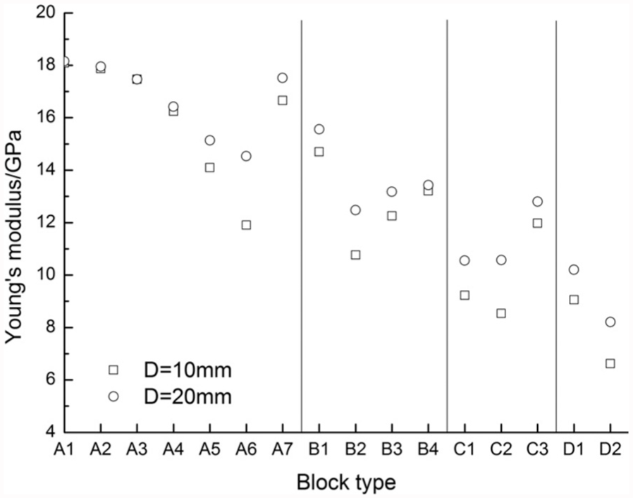
Young’s modulus of Series A_10,20, B_10,20, C_10,20 and D_10,20 under uniaxial compression.

Failure modes

Table 10 shows the failure modes of the synthetic jointed rock mass with different joint spacing. Contact force between contiguous particles in the range of x (−10, 10) and all the cracks of the whole model appearing at a certain stress state are displayed in the cross-sectional surface shown in Table 10. For each case, an image displays the bond breakage level when the stress drops to 0.8 $σ_{p}$ in the post-peak phase. As can be seen from Table 10, the joint spacing plays a major role in failure modes of rock mass under uniaxial stress. Block with single joint for every joint set is equivalent to the model with considerably great joint spacing. Joint spacing D = 10 and 20 mm is taken to investigate the effect of joint spacing on failure mode.

Table 10.

Effect of joint spacing on failure mode.

A1		A2		A3		A4
D = 20 mm	D = 10 mm	D = 20 mm	D = 10 mm	D = 20 mm	D = 10 mm	D = 20 mm	D = 10 mm

A5		A6		A7		B1
D = 20 mm	D = 10 mm	D = 20 mm	D = 10 mm	D = 20 mm	D = 10 mm	D = 20 mm	D = 10 mm

B2		B3		B4		C1
D = 20 mm	D = 10 mm	D = 20 mm	D = 10 mm	D = 20 mm	D = 10 mm	D = 20 mm	D = 10 mm

C2		C3		D1		D2
D = 20 mm	D = 10 mm	D = 20 mm	D = 10 mm	D = 20 mm	D = 10 mm	D = 20 mm	D = 10 mm

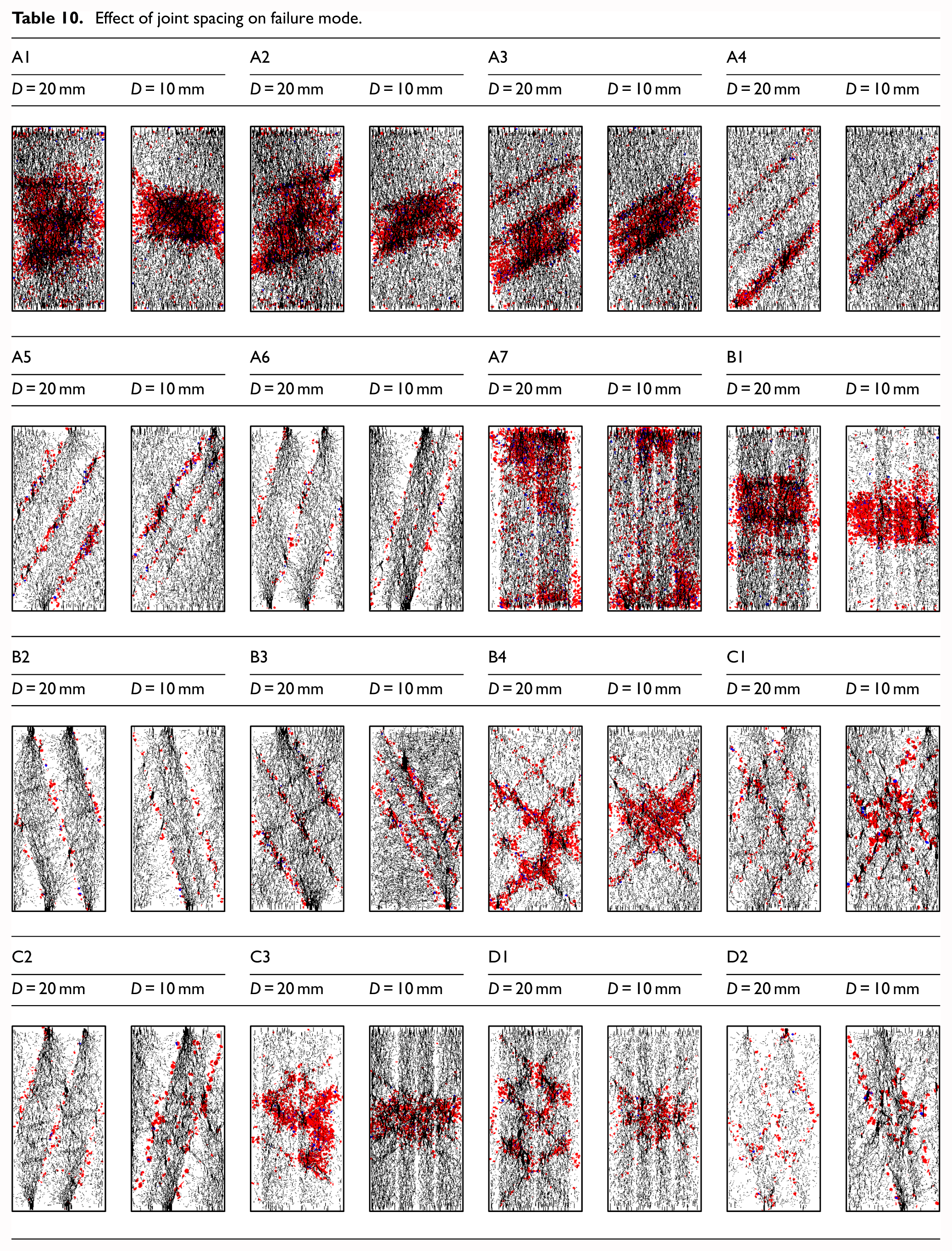
Subseries A1₁₀, A1₂₀, A2₁₀, A2₂₀, A7₁₀, A7₂₀, B1₁₀, and B1₂₀ fail in tensile splitting. It means that the joint spacing has no effect on the failure mode for the model which fails in intact failure mode. Bond breakages occur along the joint surface at the beginning for jointed block. At D = 10 mm, bond breakages along the adjacent joints more easily connect one another, and the angle between axial and failure path is relatively larger compared with D = 20 mm. It is also the reason for the reduction in strength along with the decrease in joint spacing.

Subseries A4₁₀, A4₂₀, A5₁₀, A5₂₀, A6₁₀, A6₂₀, B2₁₀, B2₂₀, B3₁₀, B3₂₀, C2₁₀, and C2₂₀ fail in planar failure mode. As same as the model failed in intact failure mode, the joint spacing has no effect on the failure mode for the above-mentioned blocks. Bond breakages on different joints do not connect each other, and it is also the micro-mechanism for the strength. As can be seen from Figure 6, for the above-mentioned blocks, the difference between the strength of blocks with different joint spacing is negligible.

Subseries A3₁₀ and A3₂₀ fail in mixed mode of tensile splitting and planar failure. Bond breakages begin to appear around the joint and extend to the intact block. Then, broken bonds between adjacent joint planes connect with the extended bond breakages. A failure plane is formed by intact failure, and joint slide appears in the model at the peak stress. At D = 10 mm, micro-cracks around the adjacent joints are more easily connected and the final failure path crossed more joints compared with those at D = 20 mm.

Subseries B4₁₀, B4₂₀, C1₂₀, C3₁₀, C3₂₀, D1₁₀, D1₁₀, D1₂₀, D2₁₀, and D2₂₀ fail under X-shaped failure mode. The similarities of the above-mentioned blocks are the multiple symmetric weak joints with opposite dip existing. When the uniaxial stress is applied on the top and bottom faces of the block, bond breakages appear along both sides of the joints. In addition, X-shaped failure occurs with the slide of crossed joints, especially for Series D as shown in Table 10.

Subseries C1₁₀ fails under step-failure mode. It is a particular case of the X-shaped failure. In this mode, a step shape failure zone is formed by broken bonds developing in the block, instead of X-shaped failure path. Therefore, step-failure mode may occur in all the above-mentioned blocks failed in X-shaped failure in theory.

Discussion of the interaction between crossed joints and stress field

Figure 9 shows the UCS of jointed models with the same weakest joint set. The UCS decreases with the increase in the number of joint sets when the dip angle of the weakest joint is in the range of 0°–45° or 80°–90°. The strength descent scope is in the range of 4–12 MPa and reached the maximum when the dip angle of the weakest joint was 30°. However, the UCS does not change significantly with the varied joint sets when the dip angle of the weakest joint was in the range of 60°–75° as Figure 9 shows. It is illustrated that the weakening action of the interaction between crossed joints on the UCS was obvious when the dip angle of the weakest joint of jointed model was in the range of 0°–45° or 80°–90°, while the weakening action is unapparent for the other jointed model. Considering numerical models A4, B4, A5, and B3 as examples, this article analyzed the influence of crossed joints on stress field and extending of cracks in the following.

Figure 9.

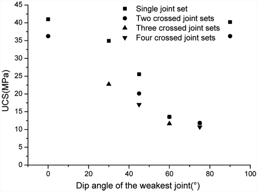
UCS of jointed samples with the same weakest joint set.

As mentioned before, numerical models in PFC3D are composed of bonded particles. Therefore, in essence, the failure of models is the destruction of parallel bonds. So, the stress field of the model can be represented by the stress state of the parallel bonds, although the parallel bonds do not transfer stress after broken. The stress state of parallel bonds in the range of x (−0.001, 0.001) was selected to represent the stress field of the total model. The normal stress and shear stress contour of Subseries A4, B4, A5, and B3 of the specified parallel bonds at corresponding peak axial stress are displayed in Figure 10. It is noted that positive sign denotes tensile for normal stress and shear stress is always positive. It is obvious that tensile stress concentration occurred in the cross position of the crossed joints in model B4, while tensile stress concentration occurred along the joint in model A4. However, the tensile stress distributions of A5 and B3 are similar. Shear stress concentration around the joints is observed in all the numerical models. It seemed that the interaction between crossed joints resulted in the tensile stress concentration when the strength of the joint sets was similar (such as A1 and B1). However, the normal stress field is not affected by the crossed joints when the strength of the joint sets varies widely (such as A2 and C3) as Figure 9 shows. It should also be noticed that the UCS of the jointed model varied slightly with the increase in joint sets when the strength of the weakest joint tended to the lowest strength level (such as A5 and C1).

Figure 10.

Stress contour for (a) normal stress and (b) shear stress.

The concentration coefficient of normal stress K_N and the concentration coefficient of shear stress K_S are defined as the ratio of maximum normal stress to axial stress and the ratio of maximum shear stress to the axial stress, respectively. The K_N and K_S of A4, B4, A5, and B3 are shown in Table 11. It is clear that both of the normal and shear stress concentration coefficients of B4 are greater than A4; nevertheless, both K_N and K_S of B3 are close to A5. It can be seen from Table 11 that the stress concentration coefficients of A5 and B3 are greater than A4 and B4, and it is the mechanical interpretation for effect of joint dip angle on the UCS of jointed rock mass. The parallel bonds of model B4 are easier to be broken than those of A4 at the same axial stress due to the stress concentration. It can also be seen in Figure 11 that the crack-initiation stress of model B4 is less than that of model A4, and the total quantity of cracks of model B4 is greater than that of model A4 under the same loading level before failure. However, the relationship of crack number to axial stress of model A5 is similar to that of model B3.

Table 11.

Concentration coefficient of A4, B4, A5, and B3.

Stress concentration coefficient	A4	B4	A5	B3
K_N	1.23	1.82	2.51	2.34
K_S	1.42	1.96	2.57	2.87

Figure 11.

The relationship of total number of cracks to axial stress.

Conclusion

BPM model using PFC3D is used to explore the effect of joint sets number and joint spacing on the mechanical behavior of a jointed rock mass under uniaxial compression. The BPM models show good agreement with physical experiments in reproducing the failure mode, UCS, and Young’s modulus under uniaxial compression.

An extensive series of numerical experiments is undertaken to investigate the effect of joint set number and joint spacing on the UCS, Young’s modulus, and failure modes. According to the results of numerical experiments, both the range and variance of UCS decreased with the increase in the joint set number. Young’s modulus of rock mass decreased with the increase in joint set number. The weaken effect of every joint set on Young’s modulus was independent, and the effect of multiple joint sets was the simple accumulation of the weaken effect of each joint set. The effect of joint orientation on failure mode depends on the number of jointed sets. It can be concluded that the effect of joint orientations on failure mode decreased with the increase in joint set number.

It is noticed that the UCS of Subseries B4 is obviously lower than Subseries A4 though they have the same joint orientation. It illustrates that the effect of crossed joint sets on the UCS of jointed rock mass is not the simple addition of the effect of each joint set. It can also be seen from the failure modes that the failure mode of Subseries B4 is X-shaped, while the failure mode of Subseries A4 is planar.

Stress concentration may occur in cross position of the model with crossed joints when the strength of the joint sets is similar. Due to the stress concentration, the strength of samples with crossed joints is relatively lower than that of samples with the single weakest joint set. The strength of samples with crossed joint sets persisted unchanged or slightly weaken when the strength of the joint sets varied widely or the strength of the weakest joint tended to the lowest strength level.

For all subseries, the UCS of jointed rock mass with three joints for each joint set is obviously greater than the UCS of jointed rock mass with single joint for each joint set. At D = 10 mm, there is a marked decrease in the UCS of jointed rock mass compared with D = 20 mm except for A3, A4, A5, A6, B2, B3, B4, C1, and C2. Furthermore, the failure modes of the above subseries are all planar or X-shaped except for A3, and do not vary with the changing joint spacing. Young’s modulus of the jointed rock mass remains unchanged with varied joint spacing when the number of joints is the same. The effect of joint spacing on Young’s modulus in this article is due to the size of model, in which partial joints cross top or bottom surface of the model. The failure mode did not change with varied joint spacing, but the failure path would be affected.

Footnotes

Acknowledgements

The authors would also like to acknowledge the editors and reviewers of this article for their very helpful comments and valuable remarks.

Academic Editor: Kai Bao

Declaration of conflicting interests

The author(s) declared no potential conflicts of interest with respect to the research, authorship, and/or publication of this article.

Funding

The author(s) disclosed receipt of the following financial support for the research, authorship, and/or publication of this article: This research is financially supported by the National Natural Science Foundation of China (Grant No. 41672258).

References

Wang

. Study on anchorage effect on fractured rock. Steel Compos Struct 2014; 17: 791–801.

Sun

Wang

. Effect of the combination characteristics of rock structural plane on the stability of a rock-mass slope. B Eng Geol Environ 2014; 73: 987–995.

Zuo

Jia

Zhu

. Numerical investigation on zonal disintegration mechanism around deep underground openings. Adv Mech Eng. Epub ahead of print 12December2013. DOI: 10.1155/2013/908028.

Jaeger

Cook

NGW

. Fundamentals of rock mechanics. 3rd ed.London: Chapman and Hall, 1979.

Duveau

Shao

JF.

A modified single plane of weakness theory for the failure of highly stratified rocks. Int J Rock Mech Min 1998; 35: 807–813.

Nassir

Settari

Wan

Joint stiffness and deformation behaviour of discontinuous rock. J Can Petrol Technol 2010; 49: 78–86.

Deere

DU.

Technical description of rock cores for engineering purposes. Rock Mech Rock Eng 1967; 1: 107–116.

Bieniawski

ZT.

Rock mass classifications in rock engineering. Int J Rock Mech Min 1976; 14: 97–106.

Barton

Lien

Lunde

Engineering classification of rock masses for the design of tunnel support. Int J Rock Mech Min 1975; 12: 189–236.

10.

Barton

Some new Q-value correlations to assist in site characterisation and tunnel design. Int J Rock Mech Min 2002; 39: 185–216.

11.

Hoek

Marinos

Benissi

Applicability of the geological strength index (GSI) classification for very weak and sheared rock masses—the case of Athens Schist formation. B Eng Geol Environ 1998; 57: 151–161.

12.

Hoek

Support of underground excavations in hard rock. New York: Taylor & Francis, 1995.

13.

Palmstrom

RMi: a rock mass characterization system for rock engineering purposes. Oslo: University of Oslo, 1995.

14.

Yang

Kulatilake

PHSW

Jing

. Numerical simulation of a jointed rock block mechanical behavior adjacent to an underground excavation and comparison with physical model test results. Tunn Undergr Sp Tech 2015; 50: 129–142.

15.

Liu

Yuan

A compressive damage constitutive model for rock mass with a set of nonpersistently closed joints under biaxial conditions. Math Probl Eng 2015; 2015: 1–10.

16.

Bahaaddini

Sharrock

Hebblewhite

BK.

Numerical investigation of the effect of joint geometrical parameters on the mechanical properties of a non-persistent jointed rock mass under uniaxial compression. Comput Geotech 2013; 49: 206–225.

17.

Singh

Rao

Ramamurthy

Strength and deformational behaviour of a jointed rock mass. Rock Mech Rock Eng 2002; 35: 45–64.

18.

Chi

Zhao

Liu

. Numerical modeling of rock fracture and fragmentation under impact loading using discrete element method. Adv Mech Eng 2015; 7: 1–5.

19.

Yang

Chen

Huang

TH.

Effect of joint sets on the strength and deformation of rock mass models. Int J Rock Mech Min 1998; 35: 75–84.

20.

Potyondy

Cundall

PA.

A bonded-particle model for rock. Int J Rock Mech Min 2004; 41: 1329–1364.

21.

Cho

Martin

Sego

DC.

A clumped particle model for rock. Int J Rock Mech Min 2007; 44: 997–1010.

22.

Kulatilake

Malama

Wang

JL.

Physical and particle flow modeling of jointed rock block behavior under uniaxial loading. Int J Rock Mech Min 2001; 38: 641–657.

23.

Kulatilake

Liang

Gao

Experimental and numerical simulations of jointed rock block strength under uniaxial loading. J Eng Mech: ASCE 2001; 127: 1240–1247.

24.

Huang

Yang

SQ.

Discrete element study on strength and failure behavior of jointed sandstone with two sets of cross-joints. J China Coal Soc 2015; 40: 76–84.

25.

Zhang

Wong

LNY

. Loading rate effects on cracking behavior of flaw-contained specimens under uniaxial compression. Int J Fracture 2013; 180: 93–110.

26.

ICG, Inc. PFC3D manual (version 4.0 ed.). Minneapolis, MN: ICG, Inc., 2008.

Mechanical and failure characteristics of rock-like material with multiple crossed joint sets under uniaxial compression

Abstract

Keywords

Introduction

Calibration of micro-parameters and validation study

Calibration of particle parameters

Calibration of joint parameters

Simulation of jointed rock mass and comparison with physical experiments

Effect of joint sets number on the mechanical properties of a jointed rock mass

UCS

Stress–strain response

Failure modes

Effect of joint spacing on the mechanical properties of a jointed rock mass

UCS

Stress–strain response

Failure modes

Discussion of the interaction between crossed joints and stress field

Conclusion

Footnotes

Acknowledgements

Declaration of conflicting interests

Funding

References