Sage Journals: Discover world-class research

Abstract

Monitoring operating vehicles’ fuel consumption and emissions is necessity for evaluating fuel saving and emissions reduction. Taxis are one of the key objects needed energy consumption monitoring in passenger transport system. However, the traditional data collection methods for vehicle fuel consumption and emissions had high cost and inconvenient maintenance. This study aims at proposing an approach to estimate taxi fuel consumption and emissions based on the global position system (GPS) trajectory data. The bench test experiment was first conducted with three different driving cycles: cruising, acceleration and deceleration, and the composite driving cycle including these two. Then, models to calculate fuel consumption and emission based on the driving trajectory reconstruction were proposed. Therefore, the taxis’ fuel consumption and emissions could be got through GPS trajectory data corresponding to these three driving cycles. The model accuracy were verified that fuel consumption (92%) and CO₂ emission (95%) fit the measurements much better than CO, NO_x, and HC emission models (60%–70%). Furthermore, taking fuel consumption per 100 km as dependent variable, the relative errors between the model’s outputs and field measurements were 1.9% in urban areas and 11.2% in comprehensive operating conditions (i.e. both urban and suburb areas).

Keywords

Global positioning system trajectory data taxi vehicle fuel consumption and emission driving cycle operating conditions

Introduction

Reducing energy consumption and emissions are of great urgent to deal with energy crisis and environmental issues worldwide. According to the government statistics reports for Beijing, the energy consumption in transportation field accounted for about 23% of the city’s total energy consumption. Specifically, due to longer operating mileages and wider coverage in urban areas, taxis should be paid more attention in energy consumption saving and emissions reduction. In order to improve fuel economy and decrease emissions in the process of operating, it is particularly necessary to monitor taxi energy consumption and emissions dynamically.

Generally, there are two approaches to test vehicle energy consumption and emissions: (1) based on controller area network (CAN) and (2) the second-by-second data detection based on oil consumption instrument. However, both these two methods require special on-board equipment, which had high cost and inconvenient maintenance. Thus, it poses a challenge for vehicle fuel consumption and emissions monitoring without additional devices mounted on vehicles. Fortunately, global position system (GPS) has been widely installed on taxis and many other operating vehicles as management requirements of vehicle tracking dynamically, safety monitoring, and real-time scheduling. Therefore, the key issue for vehicle fuel consumption and emissions monitoring could be resolved by establishing vehicle fuel consumption and emissions models based on real-time GPS trajectory data.

Hence, the current study aims at establishing fuel consumption and emissions models based on the real-time taxi GPS data, which contributing to monitor and know well the taxi’s fuel consumption and emissions in the process of operating dynamically, and further lay a foundation for transportation agencies in developing reasonable management strategies. Furthermore, there are about 66,700 registered taxis in Beijing and all of them are equipped with GPS devices, which provided good data supporting for our current study.

Literature review

In previous studies, methods for vehicle fuel consumption and emissions detection mainly included three types: bench test, remote sensing detection, and portable emission measurement system.

The bench test was usually conducted to investigate the second-by-second fuel consumption and emissions in a given driving cycle, in which the driving cycle was generally derived from the actual vehicle operational conditions in the field.^1,2 In consideration of the repeatability in the testing process, this technique was regarded as the most reliable method to measure the emissions of vehicles.³ But comparing with other test approaches, the bench test required higher cost and longer test duration.

The remote sensing detection was initially proposed by the University of Denver in 1987 and then gradually developed and applied in various countries and regions.^4–6 Due to higher automation, it could be used to collect a large amount of field emissions data at a specific location in a short time.⁷ An obvious limitation of this approach was that the detecting precision was easily affected by the surrounding environment. As only the instantaneous emissions concentration could be obtained when vehicles passed by, a new error might be caused in the process of calculating the absolute emissions quality.

Recently, portable emission measurement systems (PEMS) have been widely applied in vehicle emissions analyzing and relevant models development under different real world conditions, because of better probability, accessibility, and applicability.⁸ Based on this system, emissions for a variety of vehicle types gathered on various road types during different time periods would be collected, and further contributing to obtain emission databases for different cities.^9,10

Based on these detection methods mentioned above, a variety of fuel consumption and emissions models were developed in past years. Several models were derived from the simulation of vehicle dynamic characteristics, such as EVSIM.¹¹ For these models, the specific driving cycle was simulated by bench test, and then the parameters of vehicle operation, fuel consumption and emissions were collected for model developing. Although the accuracy was relatively higher, the applicability was reduced because of multifarious input data and complex calculation needed.

Some other researches mainly focused on the statistic models based on the relationship between vehicle operation status (e.g. speed and acceleration) and fuel consumption and emissions. By contrast, these models are more simple and fast to run. According to the sample data of instantaneous speed and acceleration collected at the Oak Ridge National Laboratory, Ahn et al.¹² proposed mixed logarithmic transformation polynomial model for fuel consumption and emissions (CO, HC, and NO_x) rate calculation. The key input variables are instantaneous speed and acceleration. Besides, Cappiello et al.¹³ established statistical fuel consumption and emissions models for light-duty vehicles based on bench tests involved more than 300 automobiles and trucks. The study results showed that the relative model error for fuel consumption and CO₂ was below 2%, and was below 10% for CO and NOx, but was not much accurate for HC. In addition, four emission ratio models were proposed by Xia:⁹ single-element regression model based on speed, emission model based on typical operation condition, bivariate regression model based on speed and acceleration, and a neural network model.

Moreover, in 1999, Luis and Palacios¹⁴ proposed the concept of vehicle specific power (VSP), which means the ratio between vehicle instantaneous output power and weight. Then VSP was widely used for studying vehicle fuel consumption and emissions. According to field test data collected by PEMS under several predetermined driving cycles, Farzaneh et al.⁸ introduced a new fuel consumption index named Base Fuel-for-Acceleration Rate (BFAR), which was defined as the amount of fuel consumption while vehicle speed increasing 1 mile/h at high speed range. BFAR could be calculated by three parameters: vehicle VSP, rated power, and speed. Besides, based on the database of fuel consumption from 26 kinds of vehicles, Xu et al.¹⁵ revealed that VSP was more relevant to fuel consumption than speed and acceleration. In his study, the VSP was divided into 42 bins by clustering analysis, and each of which corresponded to a single fuel rate. Then, Tu¹⁶ divided the speed ranges into 34 intervals, and the relationship between each speed interval and fuel rate was obtained through analyzing the percentage of VSP in each speed interval. Taking VSP as an intermediate variable, Liu¹⁰ presented a speed correction model of vehicle fuel consumption and emission rate that were suitable for diverse vehicles types on different rank roads. The result of correlation test indicated that there was a significantly linear relationship between speed and correction factors. The relative error (RE) from this correlation model was less than 20%.

Summarizing above, for vehicle fuel consumption and emissions detection, the bench test is more appropriate for a predetermined driving cycle, and the remote sensing detection is a high efficient method for emissions at a specific location, while PEMS could be used to investigate abundant realistic emissions data with lower cost. Supported by these data collection techniques, a various vehicle fuel consumption and emissions calculation models were proposed based on different theories. The simulation models based on engine power had a higher accuracy but also with intense input parameters needed, which was not much applicative. For estimating vehicle fuel consumption and emissions at specific driving patterns, statistic models depending on speed and acceleration have been approved to be highly precise. Furthermore, a good correlation between VSP and vehicle fuel consumption and emissions was found in previous studies, which contributes to establishing a relationship model between vehicle fuel consumption and emissions and variables related to VSP.

According to these above findings, this study first presented a typical taxi bench test involving three types of driving cycles: cruising driving, acceleration and deceleration and the composite driving cycle including these two cycles before. All of the three cycles were predetermined to simulate vehicle driving patterns under different operational modes. Based on the test results, the average fuel consumption and emissions (i.e. CO₂, CO, HC, and NO_x) rates on cruising pattern were obtained, and also with the mean fuel consumption and emissions in the acceleration and deceleration driving cycles. Based on driving cycles and combing the GPS data collected to generate different driving trajectories of taxis, the model of vehicle fuel consumption and emissions based on reconstruction of driving trajectory was proposed and modified. Finally, according to the simulation experiment and test in the field, the model accuracy and applicability was examined.

Experimental method

Objective

This study aims at proposing an approach to estimate the vehicle energy consumption and emissions based on the GPS trajectory data. Supported by highway traffic test field offered by the Ministry of Transport of China, the bench test experiment was first conducted to obtain vehicle fuel consumption and emissions in different driving cycles: cruising driving, acceleration and deceleration and the composite driving cycle including these two. Fuel consumption and emissions (CO₂, CO, NO_x, HC) as well as instantaneous speed and travel distance can be acquired every second by vehicle emissions testing system (VETS). According to test results of cruising and acceleration and deceleration driving cycles, models estimating taxi fuel consumption and emissions based on driving trajectory reconstruction were established. Finally, the model accuracy was calculated based on the composite driving cycle test.

Experimental designs and procedures

The experiments were conducted at Energy Testing Center of Motor Transport Industry of Ministry of Transportation, which is supported by the Ministry of Environmental Protection of China. The fuel consumption and emissions were tested on the VETS. This test system includes a 48-inch rolling drum produced by German company Schenck and an AMA-2000D emissions analyzer produced by the German company Pierburg. Through the exhaust gas analyzer, the emission values of CH, CO, and NO_x were recorded at intervals of 1 s in the process of driving, and the instantaneous fuel consumption could be calculated based on carbon balance methods.¹⁷

A Hyundai Elantra taxi was chosen as the testing vehicle in this study because of its typicality in Beijing. The testing vehicle type is BH7162AY with 1.6 L engine. The vehicle age is 5 years. According to the standard fuel consumption guided in Ministry of Industry and Information Technology of the People’s Republic of China, the fuel consumption in urban conditions is 10.7 L/100 km while is 7.6 L/100 km in comprehensive conditions.¹⁸

In Beijing, the speed limits are ranged from 30 to 120 km/h on different roadways in urban areas. Usually, the taxi driving speed is less than 95 km/h in urban conditions. Therefore, the testing speed was limited to 0–95 km/h.

Before formal test, the taxi was kept at idling for 20 min to make fuel consumption and emissions remaining at stable level. The formal test was designed to consist of three parts: cruising driving cycle test, acceleration and deceleration driving cycle test, and composite driving cycle test. These three driving tests were conducted sequentially and the engine was always alive during the interval between each test.

Cruising driving cycle

In the cruising driving cycle in the formal test, the taxi accelerated to 90 km/h gradually. In the process of cruising, the taxi kept a constant speed for 20 s when speed reached to 5, 10, 20, 30, 40, 50, 60, 70, 80, and 90 km/h. Then, the taxi was decelerated from 90 km/h to 0 km/h with the similar procedure and kept for 20 s at the corresponding speed. After these two stages, the whole cruising driving cycle was finished. To obtain stable and reliable raw data as much as possible, two same cruising driving cycles were applied for this test (i.e. the cruising test including cycles 1 and 2 in Figure 1). The total time for the cruising driving test was 1027 s. The time-speed trajectory for cruising driving test is shown in Figure 1.

Figure 1.

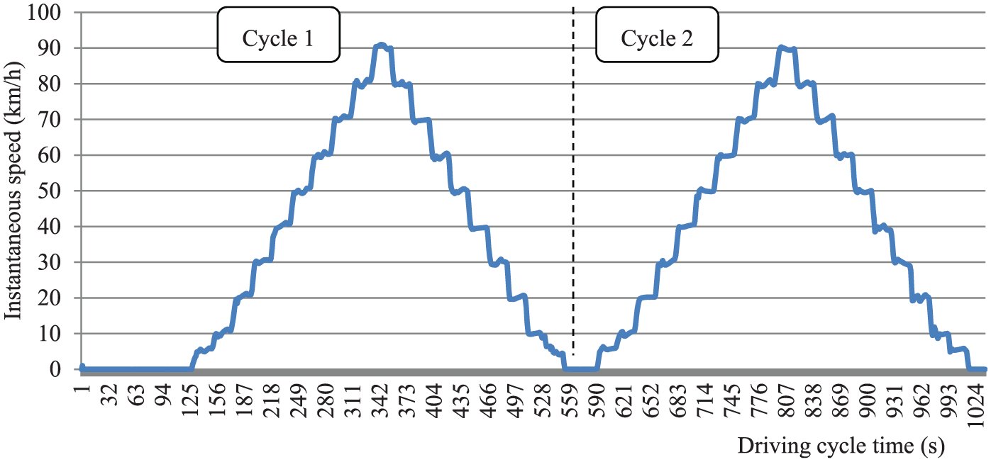
Example of time-speed trajectory of cruising driving cycle.

Acceleration and deceleration driving cycle

After cruising driving cycle, the test vehicle was kept idling for 2 min. Then, the taxi continuously accelerated from 0 to 90 km/h and then decelerated from 90 to 0 km/h in turn. After finishing these two stages, an acceleration and deceleration driving cycle was completed. Considering the randomness and diversity of driving behaviors, the acceleration and deceleration driving test was divided into three groups and each group has different values of acceleration and deceleration. For group 1, the acceleration was 1 m/s² and the deceleration is −1.4 m/s². While for groups 2 and 3, the acceleration was 0.8 and 0.6 m/s², and the deceleration is −1.4 and −1 m/s², respectively. For each group, it was conducted three times in every acceleration and deceleration driving cycle. For the whole driving test, a total time of 727 s was spent. The time-speed trajectory of acceleration and deceleration driving cycles is shown in Figure 2.

Figure 2.

Time-speed trajectory of one acceleration and deceleration driving cycle.

Composite driving cycle

To verify the accuracy of fuel consumption and emissions model proposed in our current study, the composite driving cycle tests were conducted and included three kinds of time-speed trajectories. According to the guidance in the vehicle emission standard of the People’s Republic of China Level III (i.e. Level III emission standard in European Union),¹⁹ the average operating speed is 19 km/h in light-vehicle emission tests in urban conditions. While combing with the mean driving speed from the GPS data of taxi, the average operating speeds in our study are set 29, 19, and 8 km/h, respectively. Every kind of composite driving cycle was repeated three times, and the total costing time was 1037 s. Time-speed trajectories of these three test groups are shown in Figure 3.

Figure 3.

Time-speed trajectory of composite driving cycle.

Data analysis and modeling

Fuel consumption and emissions in cruising driving cycle

As the test data was measured second-by-second and each constant speed was designed to maintain for 20 s, we obtained 20 values of fuel consumption and emissions at one set speed. For this situation, the average of every 20 measurements was illustrated, as shown in Figure 4. It is indicated that there had a high consistency for the average fuel consumption, CO₂ and CO emission rates at the same cruising speed, while big distinctions occurred for NO_x and HC at some cruising speed, especially in the first cycle. Given that there would be some random factors in the first cycle, test data extracted from the second cycle were used in the following study.

Figure 4.

Fuel consumption and emission rates in cruising driving cycle.

Obviously, in the second cycle, the average fuel consumption and emissions rates increased with speed increasing and then gradually decreased as speed reducing from 90 to 5 km/h. Meanwhile, for the same steady-state speed, the average fuel consumption and emissions rates in the first half were higher than the corresponding values in the second half. This phenomenon might be resulted from the different working states of vehicle engine during each steady-state. Based on these, mean values of the 40 instantaneous values (20 in acceleration and 20 in deceleration) at each steady-state speed in the second cycle were suggested to calculate the standard values of average fuel consumption and emissions rates. These standard values were demonstrated in Table 1.

Table 1.

Standard fuel consumption and emission rates in different cruising speed

Speed (km/h)	Mean of emissions rates
Speed (km/h)	CO₂ (g/s)	CO (g/s)	NO_x (g/s)	HC (g/s)	FUEL (L/s)
5	0.7287	0.0149	0.0013	0.0008	0.0003
10	0.9746	0.0257	0.0012	0.0012	0.0004
20	1.4375	0.0185	0.0031	0.0009	0.0006
30	1.4436	0.0250	0.0037	0.0013	0.0006
40	1.9910	0.0333	0.0062	0.0010	0.0009
50	1.9940	0.0326	0.0056	0.0010	0.0008
60	2.4130	0.0442	0.0104	0.0011	0.0010
70	2.8015	0.0708	0.0124	0.0012	0.0012
80	3.2905	0.1140	0.0163	0.0025	0.0015
90	3.7881	0.2873	0.0235	0.0061	0.0018

Fuel consumption and emissions in acceleration and deceleration driving cycle

Vehicle fuel consumption and emissions from one speed to another can be obtained based on the test data in acceleration and deceleration driving cycle. Three group tests with different accelerations and decelerations were repeated three times, respectively (see Figure 2). Thus, a total of nine group sample data were collected. The means of fuel consumption and emissions at different accelerations and decelerations were calculated and presented in Figure 5. Apparently, higher speed would result in higher fuel consumption and emission; meanwhile, various acceleration and deceleration produced significantly different fuel consumption and emissions for same speed variation in each group test. Particularly, NO_x was unsteady in acceleration process, which was inconsistent with other emissions.

Figure 5.

Fuel consumption and emissions under acceleration and deceleration driving cycle.

As shown in Figure 5, the total fuel consumption and emissions for given accelerating and decelerating process in each three group tests were not significantly different, although the acceleration and deceleration varied. It implied that the instantaneous fuel consumption and emissions per unit interval were gradually raised with the increasing of acceleration and deceleration. However, as time spending on the process of accelerating and decelerating decreased, the total values changed less obviously. As a result, the average fuel consumption and emissions were calculated as standard values for corresponding speed variation, which are summarized in Table 2.

Table 2.

Fuel consumption and emissions during different acceleration and deceleration processes.

	Speed (km/h)	CO₂ (g)	CO (g)	NO_x (g)	HC (g)	Fuel (L)
Acceleration (km/h)	5–10	7.1290	0.2416	0.0197	0.0050	0.0032
	10–20	8.7690	0.2933	0.0672	0.0051	0.0039
	20–30	14.4299	0.6634	0.0762	0.0096	0.0065
	30–40	15.0444	0.5639	0.0902	0.0137	0.0067
	40–50	21.3569	0.9491	0.1874	0.0182	0.0096
	50–60	26.2713	3.7065	0.1160	0.0456	0.0136
	60–70	26.4078	7.0210	0.1619	0.0985	0.0159
	70–80	30.1019	11.3548	0.1245	0.1481	0.0204
	80–90	37.6770	12.8391	0.1416	0.2161	0.0247
Deceleration (km/h)	90–80	6.4044	0.8621	0.0439	0.0287	0.0033
	80–70	5.1730	0.4879	0.0359	0.0184	0.0025
	70–60	4.6546	0.3256	0.0238	0.0158	0.0022
	60–50	3.6514	0.1933	0.0137	0.0122	0.0017
	50–40	2.8457	0.1102	0.0086	0.0088	0.0013
	40–30	1.9875	0.0661	0.0055	0.0064	0.0009
	30–20	1.5612	0.0466	0.0041	0.0053	0.0007
	20–10	1.3989	0.0381	0.0032	0.0049	0.0006
	10–5	1.6124	0.0406	0.0032	0.0058	0.0007

Fuel consumption and emissions in composite driving cycle

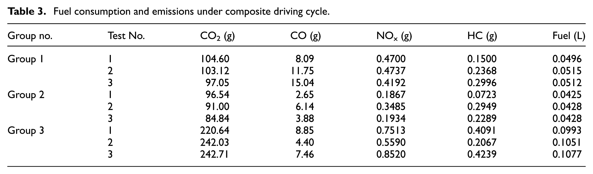
In order to validate the accuracy of models proposed in the current study, three trajectory tests in different average speeds were carried out three times, respectively (see Figure 3). Fuel consumption and emissions in these three test groups are shown in Table 3. It is indicated that the variability of fuel consumption and CO₂ emission was small, while the emissions of CO, NO_x, and HC were relatively bigger.

Table 3.

Fuel consumption and emissions under composite driving cycle.

Group no.	Test No.	CO₂ (g)	CO (g)	NO_x (g)	HC (g)	Fuel (L)
Group 1	1	104.60	8.09	0.4700	0.1500	0.0496
	2	103.12	11.75	0.4737	0.2368	0.0515
	3	97.05	15.04	0.4192	0.2996	0.0512
Group 2	1	96.54	2.65	0.1867	0.0723	0.0425
	2	91.00	6.14	0.3485	0.2949	0.0428
	3	84.84	3.88	0.1934	0.2289	0.0428
Group 3	1	220.64	8.85	0.7513	0.4091	0.0993
	2	242.03	4.40	0.5590	0.2067	0.1051
	3	242.71	7.46	0.8520	0.4239	0.1077

Additionally, according to test results of the third group in composite driving cycle (average speed = 19 km/h), the fuel consumption was calculated to be 10.32 L/100 km, which is consistent with the guidance of light-vehicle fuel consumption (10.7 L/100 km) stated by Ministry of Industry and Information Technology of the People’s Republic of China.¹⁸

Fuel consumption and emissions model

In our current study, the vehicle fuel consumption and emissions model is based on this assumption: every driving trajectory can be divided into four operating conditions, namely, idling, cruising, acceleration, and deceleration. Then, according to the GPS data and implementing trajectory reconstruction, vehicle fuel consumption and emissions could be estimated by the quantitative relationship between vehicle speed and fuel consumption and emissions in these four driving cycles. Generally, vehicles at idling status account for small proportion during a whole travel and also have low fuel consumption and emissions rates; meanwhile, it is difficult to measure the start and end time of idling through analyzing GPS trajectory data. Thus, idling condition will be regarded as one cruising part at low speed in this study.

In our current study, the cruising speed was ranged from 0 to 95 km/h. First, we divided the speed into 10 unit ranges, which were 0–5, 5–15, 15–25, 25–35, 35–45, 45–55, 55–65, 65–75, 75–85, and 85–95 km/h, respectively. To illustrate briefly, these speed ranges were simplified with the letter R and the median speed except 0–5 km/h. For example, for 15–25 km/h, it was simplified as R₂₀. Specifically, for 0–5 km/h, it was replaced by R₅. Based on this, it was presumed that the fuel consumption and emissions rates in cruising driving cycle in different speed ranges could be represented by the corresponding value in median speed. The fuel consumption and emissions of 0–5 km/h range were replaced by the value in R₅. The standard values of fuel consumption and emissions rates in cruising driving cycle are summarized in Table 1.

For acceleration and deceleration driving cycles, the fuel consumption and emissions in the process of accelerating and decelerating between these two adjacent speeds (10 given speeds stating above) were obtained through variable speed simulation experiment, as shown in Table 2. Thus, the average fuel consumption and emissions for accelerating and decelerating in a given speed interval were calculated. For the situation that the accelerating and decelerating was not in adjacent speed interval, the fuel consumption and emissions could be got by compositing the average value of multiple intervals between adjacent.

Summarizing above, vehicle fuel consumption and emissions can be estimated by adding the calculating values of cruising, acceleration and deceleration in different speed ranges together. The models of total fuel consumption and emissions based on driving trajectory reconstruction are listed as follows

T_{a} = \sum_{k} S_{k} \times t_{k} + \sum_{i} \sum_{j} C_{ij} \times P_{ij}

(1)

where T_a is the total fuel consumption and emissions (L or g); S_k is the fuel consumption and emissions rate (L/s or g/s) for different speed ranges. k values are 5, 10, 20, 30, 40, 50, 60, 70, 80 and 90; t_k is the time duration (s) in speed range k extracted from GPS trajectory data. k values are 5, 10, 20, 30, 40, 50, 60, 70, 80 and 90; C_ij is the average fuel consumption and emissions (L or g) with initial speed in range R_i and end speed in range R_j, as shown in Table 2. i, j values are 5, 10, 20, 30, 40, 50, 60, 70, 80 and 90; P_ij is the number of times when speed varied from range R_i to R_j, extracted from GPS trajectory data. i, j values are 5, 10, 20, 30, 40, 50, 60, 70, 80 and 90.

It is obvious that T_a is the total fuel consumption and emissions based on these three driving cycles. As equation (1) was proposed with an assumption that acceleration and deceleration were completed instantaneously, the calculation results would be higher than actual values. Thus, some modification was performed to remove the repeated fuel consumption and emissions in the process of accelerating and decelerating.

\begin{matrix} T = T_{a} - T_{b} = \sum_{k} S_{k} \times t_{k} + \sum_{i} \sum_{j} C_{i j} \times P_{i j} \\ - \sum_{i} \sum_{j} (S_{i} + S_{j}) / 2 \times | j - i | \times 0.46) \times P_{i j} \\ = \sum_{k} S_{k} \times t_{k} + \sum_{i} \sum_{j} (C_{i j} - (S_{i} + S_{j}) / 2 \times | j - i | \times 0.46) \times P_{i j} \end{matrix}

(2)

In equation (2), T_a is the value from equation (1). T_b is the fuel consumption and emissions in cruising process that is calculated repeatedly for accelerating and decelerating. We suppose that the acceleration and deceleration rates were 0.6 and −0.6 m/s², respectively. Then the value of 0.46 is the time required to change the speed of 1 km/h during acceleration and deceleration. Obviously, equation (2) is more reasonable than equation (1).

Model validation

Model validation for the fuel consumption and emissions included the simulation experiment and the test in the field. For the simulation experiment, the model accuracy was obtained by comparing the results between the composite driving cycles in tests and the calculation values from models. Based on different vehicle trajectories from taxi GPS data, the fuel consumption per 100 km in different running conditions was calculated, and then the model accuracy was tested through comparing with the fuel consumption per 100 km reported in official statistics.

Model validation in simulation experiment

We extracted vehicle fuel consumption and emissions in cruising, acceleration and deceleration through the second-by-second data generated in the third group of comprehensive driving cycles. Meanwhile, the vehicle trajectories were also obtained. Then, the RE of fuel consumption and emissions could be calculated by comparing the model values and test results in composite driving cycles, as shown in Table 4.

Table 4.

Relative errors between test and model results.

	Group 1 (29 km/h)		Group 2 (8 km/h)		Group 3 (19 km/h)		Comprehensive RE
	AvRE	MinRE	AvRE	MinRE	AvRE	MinRE	Comprehensive RE
FUEL	8%	4%	14%	14%	2%	0%	8%
CO₂	3%	1%	8%	2%	4%	1%	5%
CO	35%	10%	36%	11%	30%	1%	34%
NO_x	33%	26%	17%	16%	65%	33%	38%
HC	34%	7%	52%	31%	35%	19%	40%

RE: relative error.

Apparently, for test groups 1 and 3, all of the REs of fuel consumption and CO₂ emission are less than 10%. Thus, it indicated that the model has a good accuracy in calculating fuel consumption and CO₂ emission. But for test group 2, REs are higher because of low instantaneous speeds and many speed variation processes.

In addition, for each composite driving cycle tests, the model estimating results are basically same. However, as diversity of driving behaviors and operative states of engine, CO, NO_x, and HC emissions are unstable. REs are mostly concentrated between 30% and 40%, as shown in Table 4.

Model validation in field test

In order to verify the model accuracy in the field, taxi GPS data were reported at time interval of 10 s in different dates, time periods, and operation conditions. 21 times of fuel consumption based on trajectories reconstruction by the proposed model were obtained. As being restricted to the hardware facility, only fuel consumption data in the field were collected. Then, the model accuracy was obtained through comparing the fuel consumption per 100 km from model calculation results with vehicle fuel consumption statistics data.

Three Elantra taxis were chosen as test vehicles. The vehicle type was uniform and all of the vehicle models were BH7162AY with 1.6 L engine. These three vehicles were put into operation in 2011 which was controlled to have similar vehicle conditions. Figure 6 shows the GPS data of one travel returned from taxis, and its speed and time trajectory reconstructed from GPS is shown in Figure 7. Obviously, taxi trajectories can be divided into three operating conditions: cruising, acceleration and deceleration. The total fuel consumption could be calculated by equation (2), and the input relevant parameters of which were extracted from these three conditions.

Figure 6.

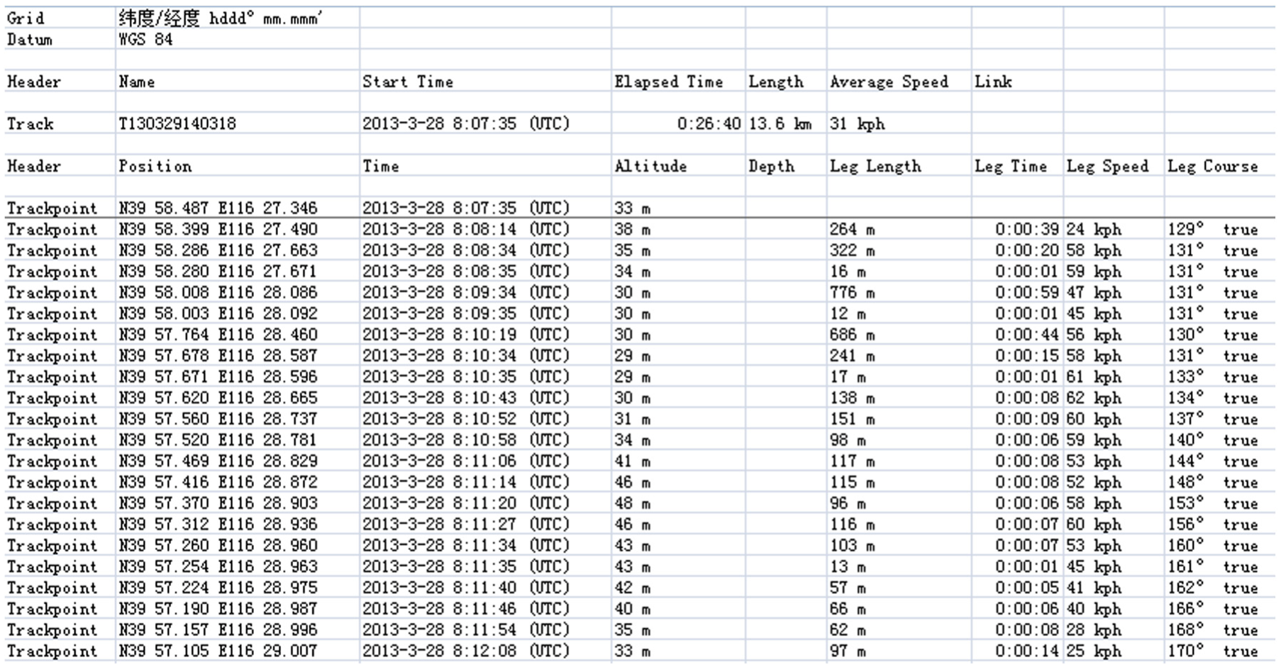
GPS sample data.

Figure 7.

Time-speed trajectory of one travel.

The distances of these 21 driving trajectories were between 3.5 and 70.3 km. Among these trajectories, there were 12 on weekdays and 9 on weekends; 14 in urban conditions and 7 in comprehensive conditions. The travel information and fuel consumption for each driving trajectory are shown in Table 5. It is clearly indicated that the fuel consumption per 100 km decreased gradually with the average speed increasing, which is in accordance with the actual situation. Furthermore, based on the average travel speed per trip listed in this table, these driving trajectories could be divided into two categories: in urban areas and in comprehensive conditions. If the mean speed was between 10 and 30 km/h, this trip was treated as urban conditions. The operation was defined as comprehensive condition when the average speed was 30–50 km/h. The comprehensive condition included both the urban and suburb areas. In addition, during the test week, the weather was good and without any adverse conditions.

Table 5.

Characteristics of travels and fuel consumption calculation results.

Serial no.	Date	Distance (km)	Average speed (km/h)	Fuel consumption (L/100 km)	Operation condition	Average fuel consumption (L/100 km)
1	Friday	18.10	13.00	13.68	Urban conditions	10.94
2	Sunday	5.71	16.30	12.36
3	Sunday	10.50	18.00	12.26
4	Friday	9.60	19.20	12.03
5	Monday	23.11	19.81	11.01
6	Wednesday	3.50	20.20	11.07
7	Friday	26.80	23.30	10.17
8	Monday	13.92	24.42	10.61
9	Sunday	34.80	24.80	10.21
10	Sunday	70.30	28.40	10.38
11	Thursday	19.20	28.90	9.43
12	Sunday	8.01	29.00	10.17
13	Sunday	12.61	29.31	9.99
14	Sunday	27.7	30.2	9.72	Comprehensive conditions	8.45
15	Saturday	37.11	35.62	10.30
16	Monday	38.70	42.60	8.51
17	Tuesday	17.70	43.60	7.52
18	Sunday	22.91	46.00	9.22
19	Thursday	18.33	46.10	8.10
20	Thursday	13.20	49.10	7.99
21	Wednesday	14.10	52.31	7.52

Based on GPS data, the fuel consumption was calculated, and the average of which is 10.94 L/100 km in urban areas and 8.45 L/100 km in comprehensive conditions. According to the official statistics from Ministry of Industry and Information Technology of the People’s Republic of China, the fuel consumption in these two conditions was 10.7 L/100 km and 7.6 L/100 km, respectively.¹⁸ Thus, the models’ REs are 1.9% and 11.2% for the two operating conditions. The analysis results indicate that our proposed model had a higher accuracy in estimating fuel consumption through GPS data returned from taxis.

Conclusion

The current study proposed models to estimate vehicle fuel consumption and emissions by reconstructing vehicle driving trajectory through second-by-second GPS data. This method provides a new solution to monitor fuel consumption and emissions dynamically.

First, the standard fuel consumption and emissions of test vehicle in cruising, acceleration and deceleration were obtained through analyzing the collection data in bench test, and which were the input parameters of proposed models. Then, based on GPS data, the driving trajectories in the field were correspondingly divided into three driving cycles of cruising, acceleration and deceleration. Thus, the total fuel consumption and emissions could be achieved using the proposed model. Several conclusions derived from the simulation experiment and test in the field could be listed as follows:

The verification results in the simulation experiment show that the model accuracy for fuel consumption and CO₂ emissions are satisfactory, the REs of which are 8% and 5%, respectively. While for emissions (i.e. CO, NO_x, and HC), the REs are between 30% and 40%.

Twenty-one driving trajectories extracted from the GPS, consisting of 14 urban conditions and 7 comprehensive conditions, were also used to verify the accuracy of the proposed model. Comparing to the fuel consumption per 100 km reported by official statistics, the model’ REs are 1.9% in urban areas and 11.2% in comprehensive running conditions. It indicates that the models based on driving trajectory reconstruction can be applicable in practical applications.

According to the model verification experiments, it was approved that the model accuracy for fuel consumption and CO₂ emission was higher, which could be used for monitoring taxis’ fuel consumption and CO₂ emission dynamically based on GPS. While for the emissions (i.e. CO, NO_x, and HC) model, it would contribute to know well the macro statistics characteristics of the emissions in taxi industry as a whole and therefore assess its environment impact.

Further research needs

Future research would be carried out in the following aspects:

Improving experiment procedures by increasing the number of test samples and repeated times; meanwhile, evaluating the influence of different driving behaviors and vehicle conditions on fuel consumption and emissions more comprehensively.

Taking vehicle emission on-board detection equipment in field tests so that contributing to verify model accuracy.

Deeply analyzing the measurement data with different processing methods and optimizing the fuel consumption and emission models.

Validating the accuracy of models by different GPS data returned frequency.

Establishing more comprehensive fuel consumption and emissions estimation models to improve applicability by considering different types of vehicles.

Footnotes

Academic Editor: Hai Xiang Lin

Author Note

Author Zhihong Chen is now affiliated with Highway Monitoring & Response Center, Ministry of Transport of P.R.C., Beijing, China.

Declaration of conflicting interests

The author(s) declared no potential conflicts of interest with respect to the research, authorship, and/or publication of this article.

Funding

The author(s) disclosed receipt of the following financial support for the research, authorship, and/or publication of this article: The authors would like to show great appreciation for the support from the Ministry of Industry and Information Technology of P. R. China under the Major Program of National Science and Technology with No. 2013ZX01045-003-002, and the National Natural Science Foundation of China (NFSC) with No. 61420106005.

References

Yanowitz

Graboski

Ryan

LBA

. Chassis dynamometer study of emissions from 21 in-use heavy-duty diesel vehicles. Envir Sci Tech 1999; 33: 209–216.

Tzirakis

Pitsas

Vehicle emissions and driving cycles: comparison of the Athens driving cycle (ADC) with ECE-15 and European Driving Cycle (EDC). Global NEST J 2006; 8: 282–290.

Durbin

Wilson

Norbeck

. Estimates of the emission rates of ammonia from light-duty vehicles using standard chassis dynamometer test cycles. Atmos Environ 2002; 36: 1475–1482.

Cadle

Stephens

RD.

Remote sensing of vehicle exhaust emission. Environ Sci Tech 1994; 28: 258A–264A.

Jiménez Palacios

Mcrae

Nelson

. Remote sensing of NO and NO₂ emissions from heavy-duty diesel trucks using tunable diode lasers. Environ Sci Tech 2000; 34: 2380–2387.

Schifter

Diaz

Duran

. Remote sensing study of emissions from motor vehicles in the metropolitan area of Mexico city. Environ Sci Tech 2003; 37: 395–401.

HJ.

Remote sensing of vehicle emissions. Environ Monitor China 2000; 16: 25–29.

Farzaneh

Zietsman

Lee

. Field evaluation and estimation method. Transport Res Rec: Transport Res Board 2009; 2001: 9–2055.

Xia

Study on light-duty vehicle microcosmic emission model on urban highway. Changchun, China: Jilin University, 2005.

10.

Liu

Speed correction model for vehicle emissions and fuel consumption based on VSP distributions. Beijing, China: Beijing Jiaotong University, 2010.

11.

Simpson

AC.

Parametric modelling of energy consumption in road vehicles. Brisbane, QLD, Australia: The University of Queensland, 2005.

12.

Ahn

Rakha

Trani

. Estimating vehicle fuel consumption and emissions based on instantaneous speed and acceleration levels. J Transport Eng 2002; 128: 182–190.

13.

Cappiello

Chabini

Nam

. A statistical model of vehicle emissions and fuel consumption. In: Proceedings of the IEEE 5th international conference, Singapore, 6 September 2002. New York: IEEE.

14.

Luis

Palacios

. Understanding and quantifying motor vehicle emissions with vehicle specific power and TILDAS remote sensing. Cambridge, MA: Massachusetts Institute of Technology, 1999.

15.

Song

. VSP-bin division for light-duty vehicles oriented to carbon dioxide. Acta Sci Circum 2010; 30: 1358–1365.

16.

On-road fuel consumption algorithm based on floating car data for light-duty vehicles. Beijing, China: Beijing Jiaotong University, 2009.

17.