On the real-time calculation of the forward kinematics of a suspended cable–driven parallel mechanism with 6-degree-of-freedom wave compensation

Abstract

A real-time forward kinematics method was proposed in this article and was used for a suspended cable-driven parallel mechanism with 6 degree-of-freedom wave compensation. The problem of the forward kinematics of a suspended cable-driven parallel mechanism was solved by a combination method including the tetrahedron approach and optimum theory. In this study, the high-dimensional nonlinear equations of mutual coupling were transformed into independent low-dimensional nonlinear equations using the tetrahedron approach. In this manner, the low-dimensional nonlinear equations could be calculated using the Levenberg–Marquardt method, thereby enabling and then, the forward kinematics could be solved in real time. Dividing the different tetrahedron solved the problem of rope slack of the redundant cable-driven parallel mechanism; therefore, this method could determine the forward kinematics of suspended cable–driven parallel mechanism just in time if the ropes were not all tensioned. Finally, an experiment was conducted on a prototype of 6-degree-of-freedom wave compensation, and the result revealed that the forward kinematics method proposed in this document was valid and accurate and could be performed in real time.

Introduction

A multi-degree-of-freedom (DOF) heaving compensation crane can compensate for the relative movement of two ships during the replenishment operation at sea, as shown in Figure 1. The suspended cable–driven parallel mechanism (SCDPM) driven by eight cables is an important part of the heaving compensation crane and can compensate for the 6-DOF motion of wave-induced ship during the replenishment operation. The SCDPM is a type of cable-driven parallel mechanism that can lift large cargo, such as containers, using cables. The mechanism has the advantages of a large working space, small inertia, and strong anti-swing ability.

Figure 1.

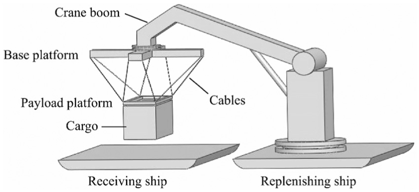
Replenishment operation at sea.

In the 80s of last century, the NIST developed the world’s first cable-driven parallel mechanism RoboCrane.^1,2 After years of research, the cable-driven parallel mechanism has made some progress in the research of kinematics,^3,4 dynamics,^5,6 tension distribution,^7,8 workspace,^9,10 and control.^11,12 In practice, it is mainly used in the fields of cargo handling,^9–11 rehabilitation robot, ¹² large spherical radio telescopes,^13,14 wave compensation,^15,16 and wind tunnel.^17,18

In the aspect of cargo handling, more and more scholars pay more attention to the attitude control of multiple DOFs. However, the work is not mature due to its complex technology. The NIST studies on the “Large Vessel Interface Lift-On/Lift-Off (LVI LO/LO) ¹⁹ ” based on the cable-driven parallel mechanism. The system can adjust the 6-DOF movement of the hoisting container by controlling the cables in the replenishment operation at sea. Lamaury et al. ²⁰ develop cable-driven parallel mechanism CoGiRo driven by eight cables with 6-DOF movement. Korayem et al.^21,22 design a 6-DOF cable-driven parallel mechanism driven by six cables. It has a similar configuration with RoboCrane. The nonlinear optimal control method is proposed by Korayem and colleagues^23,24 for the cable-driven parallel mechanism. He also makes a contribution of obtaining the maximum dynamic load-carrying capacity of planar and suspended cable-driven mechanism, ²⁵ finding the optimal trajectory for the suspended cable-driven mechanism. ²⁶ Cong et al. ²⁷ develop a cable-driven parallel mechanism with eight cables, which is used for the cargo handling and other fields. Zi et al. ²⁸ discuss the cable parallel mechanism with and without hybrid-driven planar mechanism. Qian et al.^29,30 study on the kinematics, error analysis, dynamics, and control of cable-driven parallel mechanism for multiple mobile cranes. A control method of robust iterative learning is proposed for the parallel mechanism.

There are two control schemes for SCDPM based on the coordinates used, ³¹ namely, the task and joint space coordinate. The control system controls the length of the cable obtained by sensors to reach the ideal value in the joint space coordinates, which controls the position of the end-effector.^32–34 The end-effector pose obtained from a 6-DOF position sensor or other methods is treated as a feedback for the control system in task space coordinates.^35–37 Some measure methods should be used to obtain the end-effector pose rapidly and accurately, and this is then treated as feedback for the control system in the task space control. There are many methods to measure the pose of the end-effector, namely, the computer vision,^38–40 laser sensor,^41,42 and forward kinematics (FK) method. In the replenishment operation at sea, the FK method is more suitable than other methods as control feedback method since it is not affected by weather, illumination, and other factors. However, it is necessary to ensure that the FK solution is unique and real time.

In the past, most of the relevant research studies have concentrated on the FK of 6-DOF Stewart platform. Generally, the methods reported in the literature can be classified into analytical, numerical, and sensor methods. The analytical method includes algebraic elimination, interval analysis, closed-form solutions, and polynomial equations. Algebraic elimination can be used to transform several nonlinear equations into a univariate equation. Lee and Shim^43,44 present an elimination procedure method to solve the FK problem, whereas Xu and Xi ⁴⁵ present a real-time method for a tripod FK. Huang et al. ⁴⁶ propose a closed-form FK method for a symmetrical Stewart platform based on algebraic elimination.

The interval analysis method was not able to find all of the solutions of the known search space. Merlet ⁴⁷ uses this method to compute the FK of the Gough-type mechanism. However, the computation requires a long time to complete. Innocenti ⁴⁸ solves the problem through the polynomial form method. Although the polynomial equations provide all of the solutions, the solutions are difficult to calculate because of the higher orders.

The aforementioned methods have made some progress in FK solution. Unfortunately, the end-effector pose has not been shown in a clear form so far. Moreover, because these methods generate all possible solutions, a chosen procedure is required to delete imaginary solutions while retaining real ones, which is used for the control system. In some cases, the closed-form method could provide the unique solution for the control system. Ji and Wu ⁴⁹ calculate the FK problem using the closed-form method. Fu et al. ⁵⁰ provide a closed-loop method to solve the FK problem of a special 6-DOF parallel mechanism with three limbs (TLPM). However, it is difficult for closed-form method to solve a complicated mechanism.

The numerical method includes the following: numerical iterative, neural networks, support vector machines, dual quaternion, evolutionary algorithms, and so on. The numerical iterative scheme has been the most popular approach and it could provide a unique actual solution. Yang et al. ⁵¹ put forward a FK method named modified global Newton–Raphson. Wang and Wan ⁵² propose a mixed algorithm combining immune evolutionary algorithm and numerical iterative. In that combined method, the immune evolutionary algorithm was employed to determine the approximate solution of this optimal problem in a manipulator’s workspace, with the iteration initialization selected as the last position and orientation. Pott ⁵³ proposes a method to solve the FK problem of an IPAnema cable robot using interval techniques and an iterative solver. The initial estimation was obtained by interval analysis. He also analyzed the convergence of the energy minimization method for FK to generate the starting position for the numerical optimization technique. ⁵⁴ However, an initial point sufficiently close to the solution is required in that method.

The neural network method has been studied for many years. Yee and Lim ⁵⁵ present a neural network method for the FK of a special parallel manipulator. Parikh and Lam^56,57calculate the FK problem of the parallel mechanism using the iterative neural network method in real time. Dehghani et al. ⁵⁸ use two types of neural networks, that is, multi-layer perceptron and wavelet-based neural network, to solve the FK of the HEXA mechanism. ⁵⁹ Liu et al. ⁶⁰ solve the FK problem using the neural network method. The method enables the calculation to satisfy the requirement. Ghasemi et al. ⁶¹ use the network method to solve the FK problem of an exemplary 3D cable mechanism. However, the method takes a long time to solve the FK problem and it is not suitable for real-time calculation.

The support vector machines approach is a useful data classification method. The support vector machines approach obtains the correct FK solutions in a short amount of time. Morell et al.^62,63 and Tarokh ⁶⁴ propose the method to solve the FK problem. The FK problem is solved via the classification data in the cell. The method is different from other approaches because the algorithm does not use geometric parameters. However, the memory of the control system must be large to store the off-line data, and the off-line training time is long.

Dual quaternion method will provide a unique solution if the singularity problem of the method could be solved. Yang et al. ⁶⁵ solve the full or redundancy parallel mechanism via dual quaternion method. Zhou et al. ⁶⁶ propose a FK method of Stewart platform based on the dual quaternion. However, the algorithm has not solved the singularity problem.

Evolutionary algorithm is a good choice for numerical methods. Rolland and Chandra ⁶⁷ use the evolutionary algorithm to solve the FK problems of the 6-6 parallel manipulator. Chandra and Rolland ⁶⁸ propose the memetic algorithm to solve FK problem of the 3RPR and the 6-6 leg parallel mechanism. Omran et al. ⁶⁹ use genetic method to solve the FK problem of Stewart platform. However, the algorithms will find all solutions and it is not suitable for the control system which requires a unique solution.

In addition, Wang^70,71 proposes a numerical method to solve the FK problem. This method was able to achieve a unique solution to the FK problem. He et al. ⁷² use a multi-task Gaussian process to solve the FK problem of a Stewart platform. Wang et al. ⁷³ solve the Stewart platform FK using an adaptive numerical algorithm. However, it is not suitable for the SCDPM. Gan et al.^74,75 discuss the forward displacement of the Stewart platform based on Gröbner bases.

The auxiliary sensor is a general choice to get a unique end-effector pose for the cable-driven parallel mechanism. Kim et al. ⁷⁶ propose a geometric method to solve the FK problem for a 3-SPS/S redundant manipulator based on an extra sensor. Chiu and Perng ⁷⁷ solve the FK problem in closed-form based on three redundant sensors. The use of sensor measurements^78–80 has the advantages of a short computational time and the ability to search the appropriate movements; the disadvantages are its high cost, the complexity of the measurement system, and the unavoidable round-off errors and measurement noise.

The SCDPM is different from the Stewart–Gough platform. The SCDPM is a redundant cable-driven parallel mechanism. In addition, different from the traditional rigid parallel mechanism, the SCDPM has eight cables, and the FK solution is a function of the eight variables. The process of computation is in a six-dimensional space. It is difficult to provide a unique FK solution in real time for the SCDPM since the kinematic equations are expressed as high-dimensional coupling equation. If the numerical iterative algorithm is used to calculate the FK directly, the six-dimensional matrix and the corresponding inverse matrix will be calculated at each step. It will increase the amount of calculation. Moreover, the iterative initial value is very important to the iterative algorithm. Only when the initial value is near the convergence point can the algorithm converge to the correct result.

The rope of the SCDPM will be slack in the process of control, thereby influencing the accuracy and calculation speed of the FK solution. In other words, the convergence rate is low if the rope is slack. Thus, the calculation time will be very long, thus not allowing real-time performance. Therefore, the FK of the SCDPM is more complicated to calculate because the mechanism is redundant and slack. Merlet^81,82 calculates the FK of SCDPM in real time, considering the influence of elastic and non-elastic cables. Schmidt et al. ⁸³ investigate an approach to estimate the initial value for solving the FK problem using the interval method. All of the cable-driven parallel mechanisms mentioned above are redundant. However, they do not consider the influence of the relaxation of the rope. Zhu et al. ⁸⁴ and Shao et al. ⁸⁵ study the FK problem and consider the tension states and properties of the cables in the FK model. However, it is a four-cable-driven under-constrained parallel mechanism. A FK problem of an eight-cable-driven constrained parallel mechanism has been studied in the relevant research.

In this article, a real-time calculation of the FK of the SCDPM that considers the relaxation of the rope has proposed using a combination method. The method is composed of the tetrahedral approach (TA) and the Levenberg–Marquardt (LM) method. The combination method does not require algebraic manipulation of orientation matrix elements and does not involve the high-dimensional polynomial equation. The process of the method is divided into three parts. First, in order to reduce the amount of calculation, the high-dimensional coupling equation produced by the redundant mechanism is translated into the low-dimensional decoupling equation via the TA. Second, the initial value of LM method is calculated using the approximate TA to eliminate the influence of the initial value selection of the LM method. The iteration initialization is selected as the last period initial value. Finally, the low-dimensional decoupling equations are solved using the LM method. If the relaxation rope is detected in the control, then the tetrahedral is divided again and the relaxation rope is removed from the algorithm. Next, the FK solution is calculated according to the method mentioned above. Because the high-dimensional coupling equation is translated into the low-dimensional decoupling equation and the initial value is close to the convergence point, the LM method converges rapidly, and the FK is calculated in real time.

This article contains many sections. Section “Introduction” is devoted to the basic aspects of the kinematics of the SCDPM, including a literature review and the basis of this article. Section “System description” describes the structural design and the coordinates of the SCDPM. Section “Inverse kinematics” discusses the inverse kinematics (IK) of SCDPM. Section “FK” describes the FK of the SCDPM, including the derivation of low-dimensional decoupling equation based on TA and the initial selection of the LM method. Section “The FK under the condition of rope relaxation” discusses the problem of determining how to solve the FK when the rope is slack. Section “Experiment and simulation” shows the simulation and experimental studies on solving the FK of the principal prototype. Section “Conclusion” presents the conclusions and some ideas for further work.

System description

The SCDPM is composed of the base platform end-effector and eight servo systems. The servo system is composed primarily of a servo motor, absolute encoder, tension sensor, wire rope, and corresponding mechanical system. Every two adjacent ropes are attached to a corner of the end-effector, and those ropes attached to adjacent corner of the end-effector are located close to each other, thereby increasing the working space of the SCDPM. ⁸⁶ The cable is controlled by an actuating motor. The absolute encoder measures the length of the wire rope, and the tension sensor measures the tension of the rope, as shown in Figure 2.

Figure 2.

Structure of the SCDPM.

The coordinate frame $\mathcal{N}$ is the inertial frame. The origin is placed in the inertial space. Frames $\mathcal{B}$ and $\mathcal{P}$ are placed at the base platform and the end-effector, respectively. The origin of frame $\mathcal{B}$ lies in the center of mass of the base platform, and the origin of frame $\mathcal{P}$ is located at the center of the upper surface of the end-effector.

IK

According to geometry relation shown in Figure 2, ${\mathbf{L}}_i$ is

$${\mathbf{L}}_i={\mathbf{B}}_i-({\mathbf{x}}_{\mathrm{PB}}+{\mathbf{p}}_j)$$

(1)

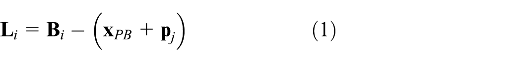
Let equation (1) for frame $\mathcal{B}$ be given by

$${\mathbf{L}}_i^B={\mathbf{b}}_i^B-({\mathbf{x}}_{\mathrm{PB}}^B+{\mathbf{R}}_P^B{\mathbf{p}}_j^P)$$

(2)

${\mathbf{p}}_i^P$ and ${\mathbf{b}}_i^B$ could be measured in the SCDPM. The constraint equations exported by equation (2) is

$$\begin{array}{l}{f^{\prime }}_i(x,y,z,\varphi ,\theta ,\psi )={\left(b_i^B-x_{PB}^B-R_P^B{p}_i^P\right)}^{\mathrm{T}}\\ \left(b_i^B-x_{PB}^B-R_P^B{p}_i^P\right)-L_i^2(i=1,\dots ,8)\end{array}$$

(3)

where $x,y,z,\varphi ,\theta ,\psi$ are the three position variables and three pose variables of the end-effector relative to the base platform, respectively; $f{\prime }_i$ is a six-dimensional nonlinear equation group that has eight equations.

If ${\mathbf{x}}_{\mathrm{PB}}^B$ and ${\mathbf{R}}_P^B$ are obtained, then the length of the ith cable is

$$\begin{array}{c}{L}_i=\left|{\mathbf{L}}_i^B\right|=\sqrt{{({\mathbf{b}}_i^B-{\mathbf{x}}_{\mathrm{PB}}^B-{\mathbf{R}}_P^B{\mathbf{p}}_j^P)}^{\mathrm{T}}({\mathbf{b}}_i^B-{\mathbf{x}}_{\mathrm{PB}}^B-{\mathbf{R}}_P^B{\mathbf{p}}_j^P)}\hfill \\ (j=1,i=1,2;j=2,i=3,4;j=3,i=5,6;j=4,i=7,8)\hfill \end{array}$$

(4)

FK

Derivation of low-dimensional decoupling equation based on TA

In this article, four real variables are used instead of the six variables of equation (3) . The eight-dimensional coupling equation is translated into the four-dimensional decoupling equation based on tetrahedron theorem, ⁸⁷ which reduces the amount of iterative computation. Then, the LM could converge rapidly to the convergence point.

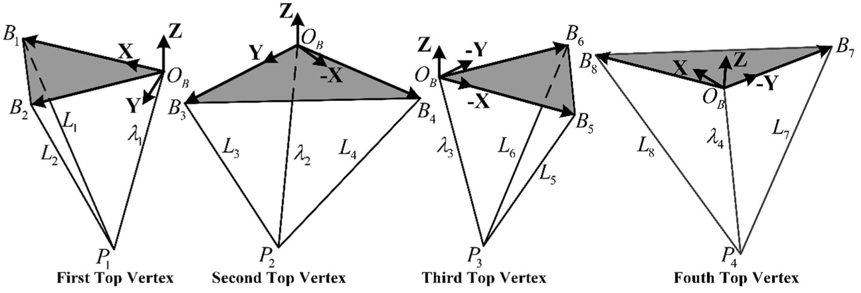
The vertices of the end-effector are treated as the top vertex of the tetrahedron. The space composed of eight ropes is divided into four tetrahedrons. The plane of the base platform is the base of the tetrahedron. The two lines that attach the same vertices of the end-effector are the space lines of the tetrahedron. The line that attaches point $O_B$ and the vertices of the end-effector is the third space line, named ${\lambda }_i$ , as shown in Figure 3.

Figure 3.

Dividing the tetrahedron.

Let the vector $\mathbf{X}\mathbf{,}\mathbf{Y}\mathbf{,}\mathbf{Z}$ be the coordinate of tetrahedron, and let $\mathbf{X}={\mathbf{B}}_1/\Vert {\mathbf{B}}_1\Vert$ , $\mathbf{Y}=(-({\mathbf{B}}_2•\mathbf{X})\mathbf{X}+{\mathbf{B}}_2)/\Vert -({\mathbf{B}}_2•\mathbf{X})\mathbf{X}+{\mathbf{B}}_2\Vert$ , and $\mathbf{Z}=\mathbf{X}\times \mathbf{Y}$ , ${\mathbf{B}}_i=\overrightarrow{O_B{B}_i}$ . The first tetrahedron includes two vertices ( $P_1$ , ${\mathbf{B}}_1$ , ${\mathbf{B}}_2$ , $O_B$ ). $P_1$ is the top vertex, and ${\lambda }_1$ is unknown, where ${\lambda }_1=\Vert {\mathbf{P}}_1\Vert$

$${\mathbf{P}}_1={\mathbf{\lambda }}_1$$

(5)

$${\mathbf{\lambda }}_1={\lambda }_{11}\mathbf{X}+{\lambda }_{12}\mathbf{Y}-{\lambda }_{13}\mathbf{Z}$$

(6)

where

$${\lambda }_{11}=\frac{{\lambda }_1^2+B_1^2-L_1^2}{2\Vert {\mathbf{B}}_1\Vert }$$

$${\lambda }_{12}=\frac{{\lambda }_1^2+B_2^2-L_2^2-2{\lambda }_{11}({\mathbf{B}}_2•\mathbf{X})}{2({\mathbf{B}}_2•\mathbf{Y})}$$

and ${\lambda }_{13}^2={\lambda }_1^2-{\lambda }_{11}^2-{\lambda }_{12}^2$ .

The second tetrahedron includes two vertices ( $P_2$ , ${\mathbf{B}}_3$ , ${\mathbf{B}}_4$ , $O_B$ ), where $P_2$ is the top vertex. ${\lambda }_2$ is unknown, where ${\lambda }_2=\Vert {\mathbf{P}}_2\Vert$

$${\mathbf{P}}_2={\mathbf{\lambda }}_2$$

(7)

$${\mathbf{\lambda }}_2={\lambda }_{21}\mathbf{Y}-{\lambda }_{22}\mathbf{X}-{\lambda }_{23}\mathbf{Z}$$

(8)

where

$${\lambda }_{21}=\frac{{\lambda }_2^2+B_3^2-L_3^2}{2\Vert {\mathbf{B}}_3\Vert }$$

$${\lambda }_{22}=\frac{{\lambda }_2^2+B_4^2-L_4^2-2{\lambda }_{21}({\mathbf{B}}_3•\mathbf{Y})}{-2({\mathbf{B}}_4•\mathbf{X})}$$

and ${\lambda }_{23}^2={\lambda }_2^2-{\lambda }_{21}^2-{\lambda }_{22}^2$ .

The third tetrahedron includes two vertices ( $P_3$ , ${\mathbf{B}}_5$ , ${\mathbf{B}}_6$ , $O_B$ ), where $P_3$ is the top vertex. ${\lambda }_3$ is unknown, where ${\lambda }_3=\Vert {\mathbf{P}}_3\Vert$

$${\mathbf{P}}_3={\mathbf{\lambda }}_3$$

(9)

$${\mathbf{\lambda }}_3=-{\lambda }_{31}\mathbf{X}-{\lambda }_{32}\mathbf{Y}-{\lambda }_{33}\mathbf{Z}$$

(10)

where

$${\lambda }_{31}=\frac{{\lambda }_3^2+B_5^2-L_5^2}{2\Vert {\mathbf{B}}_5\Vert }$$

$${\lambda }_{32}=\frac{{\lambda }_3^2+B_6^2-L_6^2+2{\lambda }_{31}({\mathbf{B}}_6•\mathbf{X})}{-2({\mathbf{B}}_6•\mathbf{Y})}$$

and ${\lambda }_{33}^2={\lambda }_3^2-{\lambda }_{31}^2-{\lambda }_{32}^2$ .

The fourth tetrahedron includes two vertices ( $P_4$ , ${\mathbf{B}}_7$ , ${\mathbf{B}}_8$ , $O_B$ ), where $P_4$ is the top vertex. ${\lambda }_4$ is unknown, where ${\lambda }_4=\Vert {\mathbf{P}}_4\Vert$

$${\mathbf{P}}_4={\mathbf{\lambda }}_4$$

(11)

$${\mathbf{\lambda }}_4=-{\lambda }_{41}\mathbf{Y}+{\lambda }_{42}\mathbf{X}-{\lambda }_{43}\mathbf{Z}$$

(12)

where

$${\lambda }_{41}=\frac{{\lambda }_4^2+B_7^2-L_7^2}{2\Vert {\mathbf{B}}_7\Vert }$$

$${\lambda }_{42}=\frac{{\lambda }_4^2+B_8^2-L_8^2-2{\lambda }_{41}({\mathbf{B}}_8•\mathbf{Y})}{2({\mathbf{B}}_8•\mathbf{X})}$$

and ${\lambda }_{43}^2={\lambda }_4^2-{\lambda }_{41}^2-{\lambda }_{42}^2$ .

${\mathbf{P}}_i$ are functions of ${\lambda }_i^2$ $(i=1,2,3,4)$ . The dot-product signs for equations (5)–(12) are determined by the angles of adjacent vectors. If the angle is an acute one, then the signs is “+”; else, it is “−”.

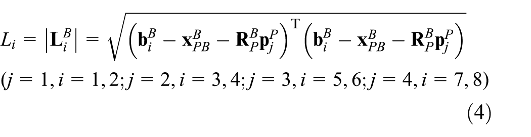
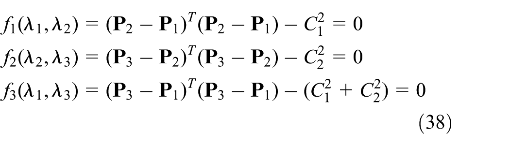
The constraint equations can be expressed as follows

$$\begin{array}{l}{f}_i({\lambda }_i,{\lambda }_j)=(P_j-P_i{)}^T(P_j-P_i)-C_i^2=0\\ (i=1,2,3,4;j=2,3,4,1)\end{array}$$

(13)

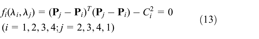
That is

$$\begin{array}{l}{f}_i({\lambda }_i,{\lambda }_j)=G_1{\lambda }_i^2+G_2{\lambda }_j^2+G_3{\lambda }_i^2{\lambda }_j^2+G_4=0\\ (i=1,2,3,4;j=2,3,4,1)\end{array}$$

(14)

where $G_i(i=1,2,3,4)$ is constant. The solution of $f_i$ is a nonlinear least squares problem. ${\lambda }_i$ $(i=1,2,3,4)$ is solved using the LM method, and the pose is solved using the geometric method.

There are four equations in $f_i$ , and each equation has only two unknown variables. Equation (14) is less variable relative to equation (3). There is no coupling between variables and no matrix operation. When $f_i$ is solved using the LM method, the objective function and gradient function can be obtained as the analytic solution compared to $f{\prime }_i$ . When the appropriate initial conditions are selected, the solution can be achieved by a finite number of iterations because the algorithm does not involve a complicated calculation, such as the inverse matrix operation. In other words, the algorithm has the characteristics of fast convergence and meets the requirement of providing a real-time solution.

Unique closed-form solution

A unique closed-form solution can be determined based on geometric method after the determination of the vector ${\mathbf{P}}_i$ .The position of the end-effector relative to the base platform $\mathbf{H}$ is

$$\mathbf{H}=[x,y,z{]}^T=\frac{{\mathbf{P}}_1+{\mathbf{P}}_2+{\mathbf{P}}_3+{\mathbf{P}}_4}{4}$$

(15)

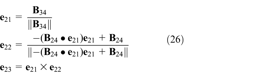
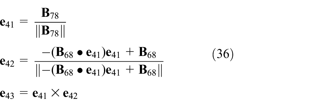
The orientation vectors $\mathbf{R}=[\mathbf{u},\mathbf{v},\mathbf{w}]$ are

$$\mathbf{u}=\frac{\frac{{\mathbf{P}}_1-{\mathbf{P}}_2}{C_1}+\frac{{\mathbf{P}}_4-{\mathbf{P}}_3}{C_3}}{2},\mathbf{v}=\frac{\frac{{\mathbf{P}}_2-{\mathbf{P}}_3}{C_2}+\frac{{\mathbf{P}}_1-{\mathbf{P}}_4}{C_4}}{2},\mathbf{w}=\mathbf{u}\times \mathbf{v}$$

(16)

$$\begin{array}{c}\varphi =\arctan (\mathbf{v}(2)/\mathbf{w}(1))\hfill \\ \theta =\arctan (-\mathbf{u}(3)/\sqrt{\mathbf{u}{(1)}^2+\mathbf{u}{(2)}^2})\hfill \\ \psi =\arctan (\mathbf{u}(2)/\mathbf{u}(1))\hfill \end{array}$$

(17)

The initial selection of the LM method

The LM method is a nonlinear least squares algorithm, which is the most widely used method by researchers. The method, which combines the advantage of the Gradient method and Newton–Raphson (NR) method, finds the maximum (minimum) value using the gradient. The key of the LM method is the initial value selection. If the initial value is too far from the convergence point, then the iteration speed is slow and may even result in no converging solution. According to the configuration characteristics of the SCDPM, this method estimates the initial value of the LM method based on the approximate TA. Next, the iteration initialization is selected as the last period initial value.

As shown in Figure 4, ${\mathbf{e}}_{\mathrm{ij}}$ $(i=1,2,3,4;j=1,2,3)$ are the coordinates of the tetrahedron. The first tetrahedron includes two vertices ( $P_1$ , ${\mathbf{B}}_{21}$ , ${\mathbf{B}}_{31}$ , $B_3$ ), where $P_1$ is the top vertex. $L_{\mathrm{est}1}$ is an unknown variable. Because the distance between $B_2$ and $B_3$ is very small in the design process, let $L_{\mathrm{est}1}\approx L_2$ in the process of solving the TA

$${\lambda }_{1\_\mathrm{int}}=\Vert {\mathbf{P}}_1\Vert$$

(18)

$${\mathbf{P}}_1={\mathbf{B}}_1+{\mathbf{L}}_1$$

(19)

$${\mathbf{L}}_1=L_{11}{\mathbf{e}}_{11}+L_{12}{\mathbf{e}}_{12}+L_{13}{\mathbf{e}}_{13}$$

(20)

where

$$\begin{array}{c}{\mathbf{e}}_{11}=\frac{{\mathbf{B}}_{21}}{\Vert {\mathbf{B}}_{21}\Vert }\hfill \\ {\mathbf{e}}_{12}=\frac{-({\mathbf{B}}_{31}•{\mathbf{e}}_{11}){\mathbf{e}}_{11}+{\mathbf{B}}_{31}}{\Vert -({\mathbf{B}}_{31}•{\mathbf{e}}_{11}){\mathbf{e}}_{11}+{\mathbf{B}}_{31}\Vert }\hfill \\ {\mathbf{e}}_{13}={\mathbf{e}}_{11}\times {\mathbf{e}}_{12}\hfill \end{array}$$

(21)

$$\begin{array}{c}{L}_{11}=\frac{L_1^2+B_{21}^2-L_2^2}{2\Vert {\mathbf{B}}_{21}\Vert }\hfill \\ L_{12}=\frac{L_1^2+B_{31}^2-L_{\mathrm{est}1}^2-2L_{11}({\mathbf{B}}_{31}•{\mathbf{e}}_{11})}{2({\mathbf{B}}_{31}•{\mathbf{e}}_{12})}\hfill \\ L_{13}^2=L_1^2-L_{11}^2-L_{12}^2\hfill \end{array}$$

(22)

${\lambda }_{1\_\mathrm{int}}$ is the initial value of ${\lambda }_1$ .

Figure 4.

The initial value of the LM method is estimated by the approximate TA.

The second tetrahedron includes two vertices ( $P_2$ , ${\mathbf{B}}_{24}$ , ${\mathbf{B}}_{34}$ , $B_4$ ), where $P_2$ is the top vertex. $L_{\mathrm{est}2}$ is an unknown variable; let $L_{\mathrm{est}2}\approx L_3$

$${\lambda }_{2\_\mathrm{int}}=\Vert {\mathbf{P}}_2\Vert$$

(23)

$${\mathbf{P}}_2={\mathbf{B}}_4+{\mathbf{L}}_4$$

(24)

$${\mathbf{L}}_4=L_{41}{\mathbf{e}}_{21}+L_{42}{\mathbf{e}}_{22}+L_{43}{\mathbf{e}}_{23}$$

(25)

where

$$\begin{array}{c}{\mathbf{e}}_{21}=\frac{{\mathbf{B}}_{34}}{\Vert {\mathbf{B}}_{34}\Vert }\hfill \\ {\mathbf{e}}_{22}=\frac{-({\mathbf{B}}_{24}•{\mathbf{e}}_{21}){\mathbf{e}}_{21}+{\mathbf{B}}_{24}}{\Vert -({\mathbf{B}}_{24}•{\mathbf{e}}_{21}){\mathbf{e}}_{21}+{\mathbf{B}}_{24}\Vert }\hfill \\ {\mathbf{e}}_{23}={\mathbf{e}}_{21}\times {\mathbf{e}}_{22}\hfill \end{array}$$

(26)

$$\begin{array}{c}{L}_{41}=\frac{L_4^2+B_{34}^2-L_3^2}{2\Vert {\mathbf{B}}_{34}\Vert }\hfill \\ L_{42}=\frac{L_4^2+B_{24}^2-L_{\mathrm{est}2}^2-2L_{41}({\mathbf{B}}_{24}•{\mathbf{e}}_{21})}{2({\mathbf{B}}_{24}•{\mathbf{e}}_{22})}\hfill \\ L_{43}^2=L_4^2-L_{41}^2-L_{42}^2\hfill \end{array}$$

(27)

${\lambda }_{2\_\mathrm{int}}$ is the initial value of ${\lambda }_2$ .

The third tetrahedron includes two vertices ( $P_3$ , ${\mathbf{B}}_{65}$ , ${\mathbf{B}}_{75}$ , $B_5$ ), where $P_3$ is the top vertex. $L_{\mathrm{est}3}$ is an unknown variable; let $L_{\mathrm{est}3}\approx L_6$

$${\lambda }_{3\_\mathrm{int}}=\Vert {\mathbf{P}}_3\Vert$$

(28)

$${\mathbf{P}}_3={\mathbf{B}}_5+{\mathbf{L}}_5$$

(29)

$${\mathbf{L}}_5=L_{51}{\mathbf{e}}_{31}+L_{52}{\mathbf{e}}_{32}+L_{53}{\mathbf{e}}_{33}$$

(30)

where

$$\begin{array}{c}{\mathbf{e}}_{31}=\frac{{\mathbf{B}}_{65}}{\Vert {\mathbf{B}}_{65}\Vert }\hfill \\ {\mathbf{e}}_{32}=\frac{-({\mathbf{B}}_{75}•{\mathbf{e}}_{31}){\mathbf{e}}_{31}+{\mathbf{B}}_{75}}{\Vert -({\mathbf{B}}_{75}•{\mathbf{e}}_{31}){\mathbf{e}}_{31}+{\mathbf{B}}_{75}\Vert }\hfill \\ {\mathbf{e}}_{33}={\mathbf{e}}_{31}\times {\mathbf{e}}_{32}\hfill \end{array}$$

(31)

$$\begin{array}{c}{L}_{51}=\frac{L_5^2+B_{65}^2-L_6^2}{2\Vert {\mathbf{B}}_{65}\Vert }\hfill \\ L_{52}=\frac{L_5^2+B_{75}^2-L_{\mathrm{est}3}^2-2L_{51}({\mathbf{B}}_{75}•{\mathbf{e}}_{31})}{2({\mathbf{B}}_{75}•{\mathbf{e}}_{32})}\hfill \\ L_{53}^2=L_5^2-L_{51}^2-L_{52}^2\hfill \end{array}$$

(32)

${\lambda }_{3\_\mathrm{int}}$ is the initial value of ${\lambda }_3$ .

The fourth tetrahedron includes two vertices ( $P_4$ , ${\mathbf{B}}_{68}$ , ${\mathbf{B}}_{78}$ , $B_8$ ), where $P_4$ is the top vertex. $L_{\mathrm{est}4}$ is an unknown variable; let $L_{\mathrm{est}4}\approx L_7$

$${\lambda }_{4\_\mathrm{int}}=\Vert {\mathbf{P}}_4\Vert$$

(33)

$${\mathbf{P}}_4={\mathbf{B}}_8+{\mathbf{L}}_8$$

(34)

$${\mathbf{L}}_8=L_{81}{\mathbf{e}}_{41}+L_{82}{\mathbf{e}}_{42}+L_{83}{\mathbf{e}}_{43}$$

(35)

where

$$\begin{array}{c}{\mathbf{e}}_{41}=\frac{{\mathbf{B}}_{78}}{\Vert {\mathbf{B}}_{78}\Vert }\hfill \\ {\mathbf{e}}_{42}=\frac{-({\mathbf{B}}_{68}•{\mathbf{e}}_{41}){\mathbf{e}}_{41}+{\mathbf{B}}_{68}}{\Vert -({\mathbf{B}}_{68}•{\mathbf{e}}_{41}){\mathbf{e}}_{41}+{\mathbf{B}}_{68}\Vert }\hfill \\ {\mathbf{e}}_{43}={\mathbf{e}}_{41}\times {\mathbf{e}}_{42}\hfill \end{array}$$

(36)

$$\begin{array}{c}{L}_{81}=\frac{L_8^2+B_{78}^2-L_7^2}{2\Vert {\mathbf{B}}_{78}\Vert }\hfill \\ L_{82}=\frac{L_8^2+B_{68}^2-L_{\mathrm{est}4}^2-2L_{81}({\mathbf{B}}_{68}•{\mathbf{e}}_{41})}{2({\mathbf{B}}_{68}•{\mathbf{e}}_{42})}\hfill \\ L_{83}^2=L_8^2-L_{81}^2-L_{82}^2\hfill \end{array}$$

(37)

${\lambda }_{4\_\mathrm{int}}$ is the initial value of ${\lambda }_4$ .

The FK under the condition of rope relaxation

The significant difference among the cable-driven parallel mechanisms is that the rope may relax during the control process. Because the parallel mechanism involves redundant actuation, the probability of rope relaxation is high. When the rope is slack, the length of the rope will be longer. Next, the error will influence the accuracy and convergence speed in the iterative process, which does not meet the accuracy and real-time requirements. Therefore, the rope relaxation should be considered in the process of solving the FK of the SCDPM. Only when the number of the rope tension is greater than or equal to six can the SCDPM control the end-effector perform a 6-DOF movement. The six, seven, and eight states of the rope tension are considered in this study. The situation is divided into the following types.

The “2220” and “2221” types

If the two ropes connecting one vertex of the end-effector with the base platform are all under tension, then the rope tension value is “2.” If one of the ropes is under tension and the other is slack, then it is “1.” If the two ropes are all slack, then it is “0.”“2220” indicates that the two ropes connecting one vertex are all slack, and that the remaining ropes are all under tension. “2221” indicates that only one of the ropes is slack and the rest are all under tension. Because a plane can be determined by the three non-collinear points, the pose of end-effector can be solved by only calculating the coordinate of the three “2” vertex of the end-effector using the LM method. The ropes connecting the fourth vertex of the end-effector are not considered, regardless of the “1” or “0” cases. For example, the ropes $L_7$ and $L_8$ are either all slack or one of the two ropes is slack. The ${\mathbf{\lambda }}_i(i=1,2,3)$ is calculated using equations (5)–(10), and the constraint equations are

$$\begin{array}{c}{f}_1({\lambda }_1,{\lambda }_2)=({\mathbf{P}}_2-{\mathbf{P}}_1{)}^T({\mathbf{P}}_2-{\mathbf{P}}_1)-C_1^2=0\hfill \\ f_2({\lambda }_2,{\lambda }_3)=({\mathbf{P}}_3-{\mathbf{P}}_2{)}^T({\mathbf{P}}_3-{\mathbf{P}}_2)-C_2^2=0\hfill \\ f_3({\lambda }_1,{\lambda }_3)=({\mathbf{P}}_3-{\mathbf{P}}_1{)}^T({\mathbf{P}}_3-{\mathbf{P}}_1)-(C_1^2+C_2^2)=0\hfill \end{array}$$

(38)

${\lambda }_i$ $(i=1,2,3)$ is solved using the LM method, and the position of the end-effector relative to the base platform $\mathbf{H}$ is

$$\mathbf{H}=[x,y,z{]}^T=\frac{{\mathbf{P}}_1+{\mathbf{P}}_3}{2}$$

(39)

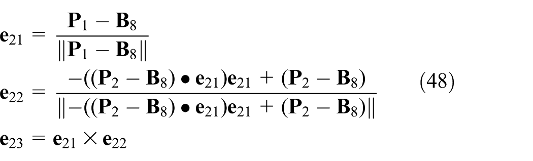
The orientation vectors $\mathbf{R}=[\mathbf{u},\mathbf{v},\mathbf{w}]$ is

$$\mathbf{u}=\frac{{\mathbf{P}}_1-{\mathbf{P}}_2}{C_1},\mathbf{v}=\frac{{\mathbf{P}}_2-{\mathbf{P}}_3}{C_2},\mathbf{w}=\mathbf{u}\times \mathbf{v}$$

(40)

The “2211” type

“2211” indicates that there are two relaxation ropes distributed in two vertices of the end-effector. This type is based on the following: the coordinate of the two “2” vertex is calculated using the LM method, and the vector of the two “2” vertex is known. Next, the other two coordinates of the “1” vertex are calculated using the vector of the two “2” vertices. For example, if $L_5$ and $L_7$ are slack, then the tetrahedron is divided again, as shown in Figure 5.

Figure 5.

The tetrahedron dividing the “2211” type.

The first and second tetrahedron is the same as those in Figure 4. ${\mathbf{P}}_1$ and ${\mathbf{P}}_2$ are calculated using equations (5)–(8). The constraint equation is

$$f_1({\lambda }_1,{\lambda }_2)=({\mathbf{P}}_2-{\mathbf{P}}_1{)}^T({\mathbf{P}}_2-{\mathbf{P}}_1)-C_1^2=0$$

(41)

${\mathbf{\lambda }}_1$ and ${\mathbf{\lambda }}_2$ are calculated using the LM method. ${\mathbf{P}}_1$ and ${\mathbf{P}}_2$ are calculated according to ${\mathbf{\lambda }}_1$ and ${\mathbf{\lambda }}_2$ . The third tetrahedron includes two vertices ( $P_3$ , $\overrightarrow{B_6{P}_1}$ , $\overrightarrow{B_6{P}_2}$ , $B_6$ ), where $P_3$ is the top vertex

$${\mathbf{P}}_3={\mathbf{B}}_6+{\mathbf{L}}_6$$

(42)

$${\mathbf{L}}_6=L_{61}{\mathbf{e}}_{11}+L_{62}{\mathbf{e}}_{12}-L_{63}{\mathbf{e}}_{13}$$

(43)

where

$$\begin{array}{c}{\mathbf{e}}_{11}=\frac{{\mathbf{P}}_1-{\mathbf{B}}_6}{\Vert {\mathbf{P}}_1-{\mathbf{B}}_6\Vert }\hfill \\ {\mathbf{e}}_{12}=\frac{-(({\mathbf{P}}_2-{\mathbf{B}}_6)•{\mathbf{e}}_{11}){\mathbf{e}}_{11}+({\mathbf{P}}_2-{\mathbf{B}}_6)}{\Vert -(({\mathbf{P}}_2-{\mathbf{B}}_6)•{\mathbf{e}}_{11}){\mathbf{e}}_{11}+({\mathbf{P}}_2-{\mathbf{B}}_6)\Vert }\hfill \\ {\mathbf{e}}_{13}={\mathbf{e}}_{11}\times {\mathbf{e}}_{12}\hfill \end{array}$$

(44)

$$\begin{array}{c}{L}_{61}=\frac{L_6^2+{({\mathbf{P}}_1-{\mathbf{B}}_6)}^2-(C_1^2+C_2^2)}{2\Vert {\mathbf{P}}_1-{\mathbf{B}}_6\Vert }\hfill \\ L_{62}=\frac{L_6^2+{({\mathbf{P}}_2-{\mathbf{B}}_6)}^2-C_2^2-2L_{61}(({\mathbf{P}}_2-{\mathbf{B}}_6)•{\mathbf{e}}_{11})}{2(({\mathbf{P}}_2-{\mathbf{B}}_6)•{\mathbf{e}}_{12})}\hfill \\ L_{63}^2=L_6^2-L_{61}^2-L_{62}^2\hfill \end{array}$$

(45)

where ${\mathbf{\lambda }}_1={\mathbf{P}}_1$ and ${\mathbf{\lambda }}_2={\mathbf{P}}_2$ . The fourth tetrahedron includes four vertices ( $P_4$ , $\overrightarrow{B_8{P}_1}$ , $\overrightarrow{B_8{P}_2}$ , $B_8$ ), where $P_4$ is the top vertex

$${\mathbf{P}}_4={\mathbf{B}}_8+{\mathbf{L}}_8$$

(46)

$${\mathbf{L}}_8=L_{81}{\mathbf{e}}_{21}+L_{82}{\mathbf{e}}_{22}-L_{83}{\mathbf{e}}_{23}$$

(47)

where

$$\begin{array}{c}{\mathbf{e}}_{21}=\frac{{\mathbf{P}}_1-{\mathbf{B}}_8}{\Vert {\mathbf{P}}_1-{\mathbf{B}}_8\Vert }\hfill \\ {\mathbf{e}}_{22}=\frac{-(({\mathbf{P}}_2-{\mathbf{B}}_8)•{\mathbf{e}}_{21}){\mathbf{e}}_{21}+({\mathbf{P}}_2-{\mathbf{B}}_8)}{\Vert -(({\mathbf{P}}_2-{\mathbf{B}}_8)•{\mathbf{e}}_{21}){\mathbf{e}}_{21}+({\mathbf{P}}_2-{\mathbf{B}}_8)\Vert }\hfill \\ {\mathbf{e}}_{23}={\mathbf{e}}_{21}\times {\mathbf{e}}_{22}\hfill \end{array}$$

(48)

$$\begin{array}{c}{L}_{81}=\frac{L_8^2+{({\mathbf{P}}_1-{\mathbf{B}}_8)}^2-C_4^2}{2\Vert {\mathbf{P}}_1-{\mathbf{B}}_8\Vert }\hfill \\ L_{82}=\frac{L_8^2+{({\mathbf{P}}_2-{\mathbf{B}}_8)}^2-(C_1^2+C_2^2)-2L_{81}(({\mathbf{P}}_2-{\mathbf{B}}_8)•{\mathbf{e}}_{21})}{2(({\mathbf{P}}_2-{\mathbf{B}}_8)•{\mathbf{e}}_{22})}\hfill \\ L_{83}^2=L_8^2-L_{81}^2-L_{82}^2\hfill \end{array}$$

(49)

The position and pose of the end-effector relative to the base platform are calculated using equations (15)–(17).

Experiment and simulation

The principle prototype of SCDPM is shown in Figure 6(a). The end-effector driven by eight cables can move with six DOF. The measurement system consists of eight absolute encoders, three laser sensors, and one inertial measurement units (MTi). Every absolute encoder installed in the base platform detects the length of cables. The controller solves the FK problem according to the length using the method proposed in this article. The installation positions of the three laser sensors are shown in Figure 6(a), and the second and third laser sensors are blocked by the base platform. The laser sensor detects the distance between the end-effector plane and the laser sensor. That is, the displacement of swaying, surging, and heaving. They are used to verify the accuracy of the FK solution in these directions. The MTi is installed on the end-effector, as shown in Figure 6(a). The MTi detects the pose of the end-effector, namely, pitching, rolling, and yawing. The results are compared with the FK.

Figure 6.

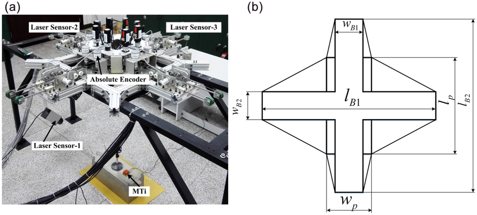
(a) Principle prototype of SCDPM and (b) geometric parameters of the system.

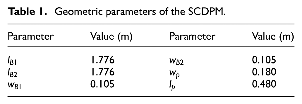
The geometric notation is shown in Figure 6(b). The structural parameter of SCDPM is shown in Table 1. The control system is established based on C++ language. The FK program is written using MATLAB. Next, the control system calls the LIB, DLL, and H files produced by MATLAB in real time to solve the problem. The CPU is an Intel i5-4460 operating at 3.20 GHz.

Table 1.

Geometric parameters of the SCDPM.

Parameter	Value (m)	Parameter	Value (m)
$l_{B1}$	1.776	$w_{B2}$	0.105
$l_{B2}$	1.776	$w_p$	0.180
$w_{B1}$	0.105	$l_p$	0.480

First, the effect of the initial value of the LM method on the FK is analyzed. Next, the simulation of FK in the Mode of “2222” has been researched. Finally, the experiment has been conducted on the prototype of the SCDPM. The FK is solved in real time in the states of “2222,”“2220,” and “2211.”

Effect of the initial value of the LM method on the FK

The ideal initial value of the LM method calculated by the prototype is ${\lambda }_{\mathrm{ideal}\_\mathrm{int}}=1.1246m$ . To analyze the effect of different initial values on the FK in the three states, the simulation analysis is performed using MATLAB. The pose is set as $\mathrm{Pose}=[20\sin (0.1t),0,0{]}^T(t=0,1,2,\dots )$ and the position is set as $\mathrm{Position}=[0,0,-1.095{]}^T$ ; the initial values considered are $\lambda =1.1m$ , $\lambda =1.05m$ , $\lambda =1.0m$ , and $\lambda =0.95m$ . The results are shown in Table 2.

Table 2.

Effect of the initial value of the LM method on the forward kinematics.

Initial value	2222	2220	2211
$\lambda =1.1m$	✓	✓	✓
$\lambda =1.05m$	✓	✓	✓
$\lambda =1.0m$	✓	✓	✗
$\lambda =0.95m$	✓	✗	✗

✓

—the FK result converges to the set path.

✗

—the FK result does not converge to the set path.

As shown in Table 2, the FK result converges to the set path with all initial values in the “2222” model. However, the FK result does not converge to the set path with the initial value of 0.95 in the “2220” model. The “2211” model does not converge to the set path with the initial values of 1.0 and 0.95. It is concluded that the “2222” model is least sensitive to the initial value, and that the “2211” model is most sensitive to the initial value. A horizontal comparison reveals that the robustness of the FK to the selection of the initial value is improved with the increase of the constraint equation. Therefore, the control system of SCDPM should avoid the situation of slack rope. A longitudinal comparison shows that the closer to the ideal initial value, the easier it is for the model to converge. The initial value of this article is related to the value of $w_{B1}$ and $w_{B2}$ , according to the previous method; the smaller the two values are, the closer the initial value is to the ideal value. Therefore, in the design process, the two values should be minimized to make its initial value close to the ideal value. The initial value of this article is 1.0954, and the three models used are all convergent.

Simulation of FK in the mode of “2222”

The IK produces 100 groups of data of cable length in each direction using equation (4). In the “2222” model, solutions of FK problem in the six directions have been studied by simulation based on the FK method proposed in this article. The termination threshold of the LM algorithm is chosen to be 10⁻⁶. The maximum number of iterations is set to 50. The result of the error between the FK and the model, the distribution of number of iterations, and density distribution of the iteration time for each group of data are shown in Figures 7–9.

Figure 7.

The error of each group of data in six directions: (a) shows the position error in the directions of swaying, surging and heaving and (b) shows the pose error in the directions of pitching, rolling and yawing.

Figure 8.

The distribution of number of iterations in six directions: (a) shows the histogram of the number of iterations in three position directions and (b) shows the histogram in three pose directions.

Figure 9.

The density distribution of iteration time in six directions: (a)–(f) show the density distribution of iteration time in the directions of swaying, surging, heaving, pitching, rolling and yawing, respectively.

Figure 7(a) shows the position error and Figure 7(b) shows the pose error. It can be concluded from Figure 7 that the position error is less than 10⁻⁶ m, and the pose error is less than 10⁻⁴°.

Figure 8(a) shows the histogram of the number of iterations in three position directions. Figure 8(b) shows the histogram in three pose directions. As shown in Figure 8, the iteration number of most of groups is the 2 step in the direction of swaying. The same result is also found in the directions of surging and rolling. The number of iterations is about half of the 2 step, half of the 3 step in heaving. The iteration number of most of groups is the 3 step in pitching and only one step occurs in yawing.

As shown in Figure 9, the more the number of iterations, the more time it takes to solve. The iteration time of per group of data is about 1 ms in the direction of yawing. The iteration time is about 2 ms in pitching and 1–2 ms in other directions. Due to the lack of high precision clock in the Windows operating system, it is difficult to distinguish the time under 1 ms. Therefore, there is a certain error between the simulation time and the actual iteration time.

In order to further illustrate the superiority of the method proposed in this article, the solution solved by the method of TA and LM is compared with the solution solved by LM method ⁵³ directly. The results are shown in Table 3.

Table 3.

Comparison of two methods.

	TA + LM	LM directly
Number of variables	4	6
Number of equations	4	8
Method of initial value estimation	Approximate TA	Interval method
Number of cables	8	8
Degrees of freedom	6	6
Position error	<10−6 m	<10−4 m
Pose error	<10−4°	–
Number of iterations	2–3	8–15

TA: tetrahedral approach; LM: Levenberg–Marquardt.

It can be concluded that the precision of the method proposed in this article is higher than the method using LM directly. Because of the low-dimensional equation obtained by TA, the computational cost is not only reduced, but also the number of iteration steps is reduced.

Experiment of FK in the models of “2222,”“2220,” and “2211”

In the “2222” model, all the cables are under tension. The solution result of the FK, the laser sensor, the MTi, the number of iterations, and the length of cables are shown in Figures 10–12.

Figure 10.

The FK result in the model of “2222”: (a) the position of the end-effector is solved by the FK method and laser sensor and (b) the pose of the end-effector is solved by the FK method and MTi.

Figure 11.

Lengths of the cables for translational motion in the model of “2222”: (a)–(h) the lengths of the cables for translational motion in the model of “2222”, respectively.

Figure 12.

Lengths of the cables for rotational motion in the model of “2222”: (a)–(h) the lengths of the cables for rotational motion in the model of “2222”, respectively.

As shown in Figure 10, the red line is the position or poses of the end-effector solved by the FK method proposed in this article. The green line is the position or poses of the end-effector measured by the laser sensor or MTi. Figure 10(a) shows that the position of the end-effector could be solved by the FK method, and the FK solution curve is smooth and its performance is similar to the laser sensor. Figure 10(b) shows that the pose of the end-effector could be solved by the FK method, and then the FK solution is similar to those of the MTi. It is obvious that the FK problem could be solved in real time when all of the cables are under tension.

Figure 11(a)–(h) represents the lengths of the cables $l_i(i=1,\dots ,8)$ for translational motion in the model of “2222,” respectively. It shows that all eight cables are driven to make the periodic motion with end-effector during the process of control. All cables remain in a tight state for translational motion in the model of “2222.”

Figure 12(a)–(h) represents the lengths of the cables $l_i(i=1,\dots ,8)$ for rotational motion in the model of “2222,” respectively. It shows that all eight cables are driven to make the periodic motion with end-effector. All cables remain in a tight state for rotational motion in the model of “2222.”

The cable $L_7,L_8$ is slack, whereas the other six cables remain under tension. The experimental results of the translational motion and the rotational motion are shown in Figure 13.

Figure 13.

The FK result in the model of “2220”: (a) the position of the end-effector is solved by the FK method and laser sensor and (b) the pose of the end-effector is solved by the FK method and MTi.

The red line is the position or poses solved by the FK method proposed. The green line is the position or poses measured by the laser sensor or MTi. Figure 13(a) shows that the position of the end-effector could be solved by the FK method in the model of “2220.” The performance of FK solution is similar to the laser sensor. Figure 13(b) shows that the end-effector pose could be solved by the FK method in the model of “2220.” The FK solution is similar to those of the MTi. Figure 13 shows that the FK problem could be solved in real time in the model of “2220.”

The cable $L_5,L_7$ is slack, whereas the other six cables remain under tension. The experiment results of translational motion and rotational motion are shown in Figure 14.

Figure 14.

The FK result in the model of “2211”: (a) the position of the end-effector is solved by the FK method and laser sensor and (b) the pose of the end-effector is solved by the FK method and MTi.

The red line is the position or poses solved by the FK method proposed. The green line is the position or poses measured by the laser sensor or MTi. Figure 14(a) shows that the end-effector position could be solved by the FK method in the model of “2211.”Figure 14(b) shows that the end-effector pose could be solved by the FK method in the model of “2211.”Figure 14 shows that the FK problem could be solved in real time in the model of “2211.”Figures 13 and 14 show that the method proposed in this article can also solve the positive solution in real time in the case of rope slack.

Figure 15 shows the distribution of number of iterations in the model of 2222, 2220, and 2211. It is obtained that the iteration number of “2222” model is higher than those of the other two models because the “2222” model has more constraint equations. The fewer constraints there are, the fewer number of iterations and, thus, the shorter the computational time will be. However, it can be seen from the above that the less constrained model is less robust. The computation time is inversely proportional to the robustness.

Figure 15.

The distribution of number of iterations in the model of 2222, 2220, and 2211.

Conclusion

In this article, the real-time calculation of the FK of SCDPM is solved using the tetrahedral method and the LM method. The FK problem can be calculated, regardless of whether the cables are slack or under tension. The combination method does not require algebraic manipulation of orientation matrix elements and does not involve the high-dimensional polynomial equation. The reason is that the high-dimensional coupling equation is translated into the low-dimensional decoupling equation via the TA. Therefore, the amount of computation is reduced, and the FK can be solved in only 2–3 step. The position error is 10⁻⁶ m and the pose error is 10⁻⁴°. The FK method proposed in this article could precisely solved the FK problem of the SCDPM in real time.

In addition, the initial value of LM method is calculated using the approximate TA to eliminate the influence of the initial value selection of the LM method. The law between the initial value and the constraint equations is revealed: the more constraint equations are used, the higher the robustness is. On one hand, increasing the number of constraint equations increases the number of iteration steps. On the other hand, fewer constraint equations and fewer iteration steps may cause low robustness and poor stability. The smaller the values of $w_{B1}$ and $w_{B2}$ are, the closer the initial value of LM is to the ideal value, and the higher the robustness is.

The FK method proposed in this article is only applicable to the type of mechanism with two cables connected to the same point of the end-effector and the geometric parameters of the mechanism must be known. In the process of solving the problem, there is a certain noise in the rope length measurement. In practice, there is a certain noise cable length measurement. In this article, the influence of the change in cable length on the precision and time is not considered. Moreover, the number of FK solutions of this configuration has not been studied. In the further work, the influence of the change in cable length on the FK problem and the number of FK solutions will be carried out.