
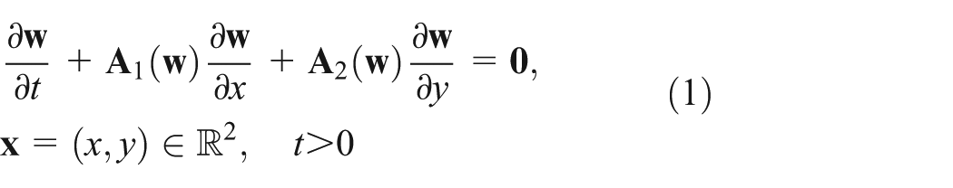
Abstract
The purpose of this article is to demonstrate that the discontinuous Galerkin method is efficient and suitable to solve linearized Euler equations, modelling sound propagation phenomena. Several benchmark problems were chosen for this purpose. We studied the effect of the underlying computational mesh on the convergence rate and showed the importance of high-quality meshes in order to achieve the theoretical convergence rates. Various acoustic boundary conditions were examined. Perfectly matched layer was used as a non-reflecting boundary condition.
Keywords
Introduction
The linearized Euler equations (LEE) are often used as the mathematical model to simulate acoustic propagation. An alternative to the LEE is the acoustic perturbation equation (APE). 1 High-order methods are necessary to achieve the desirable accuracy of acoustic simulations. The discontinuous Galerkin method (DGM) therefore seems ideal for the spatial discretization of the LEE. It allows one to reach high-order accuracy while maintaining the ability to deal with complex geometries. This is achieved by combining features of the finite element method (high-order solution) and finite volume method (local element-based solution). The DGM was first introduced in Cockburn and Shu 2 and has been since developed for hyperbolic systems. The first successful application of the DGM was presented in Reed and Hill 3 to solve the neutron transport equation. Examples of the successful application of DGM to acoustic problems are Reymen et al. 4 or Bauer et al. 5 In Reymen et al., 4 the DGM was applied to three-dimensional (3D) acoustic pulse propagation problem to analyse the convergence rate of the method. In Bauer et al., 5 the DGM was applied to solve two-dimensional (2D) APE-4 for monopole in boundary layer problem. Our aim is to test the DGM for several 2D benchmark problems with various boundary conditions (BCs). Additionally, different meshing algorithms were tested to analyse the effect of the computational mesh on the convergence rate of the method.
Outline
The article is organized as follows. In section ‘LEE’, the 2D LEE are derived from the more general Euler equations (EE). Section ‘Discretization’ describes the nodal DGM, which is used for the spatial discretization of the LEE, as well as the specification of numerical flux. Numerical flux is one of the most important aspects of this method and a common feature of the DGM and the finite volume method. It is the numerical flux that allows us to describe the dynamics of the system under consideration. We then turn our attention to time discretization, where we utilize the explicit Runge–Kutta method to perform time integration. The effect of the underlying mesh used for computation is also discussed. Experimenting with different meshes revealed that the theoretical convergence rate
The second part of this article is devoted to applying the DGM to acoustic simulations. We chose a simple acoustic pulse propagation problem as a benchmark problem to demonstrate the high-order nature of this algorithm. We also test the effectiveness of the BC used, namely, reflecting BC and non-reflecting BC (NRBC). The latter is used to simulate the propagation of acoustic waves in a truncated domain to ensure that the outgoing waves do not reflect back to the computational domain. One of the most promising approaches to implement NRBC is the perfectly matched layer (PML), which was first formulated in Hu 6 for LEE. It was found that this formulation had stability issues, and stable formulation for uniform mean flow was presented in Hu 7 and extended to non-uniform mean flow in Hu. 8 This approach was later extended to full EE and Navier–Stokes equations (cf. Hu et al. 9 ).
LEE
This section is devoted to the derivation of the 2D LEE. They are obtained by linearizing the EE written in primitive variables (density
where

and
We assume that the variables can be decomposed into two parts – the reference state (sometimes called mean value) and fluctuations (or perturbations) – in the following way

where variables with the subscript ‘
We assume that the magnitudes of the fluctuations are very small compared to those of the mean values, that is

Therefore, we can approximate the matrices

Inserting approximation (4) into EE (1), we obtain the LEE

where

If we consider uniform flow, that is, the mean values are constant in space, the term
Discretization
This section deals with discretization techniques used to solve the LEE. The DGM is a suitable method for solving the LEE because the LEE represents conservation laws of mass, momenta and energy, and the DGM is capable of respecting these laws on individual mesh elements with high order. In contrast to the standard dispersion-relation-preserving finite difference schemes for computational acoustics (cf. Tam and Webb 11 ), the DGM is able to handle complex geometries.
Spatial discretization
The algorithm we use is based on the nodal DGM described in Hesthaven and Warburton
12
extended to the case of the LEE. We use the quadrature-free implementation as proposed in Atkins and Shu
13
to avoid numerical integration. The algorithm is presented for the LEE with
We suppose that the computational domain
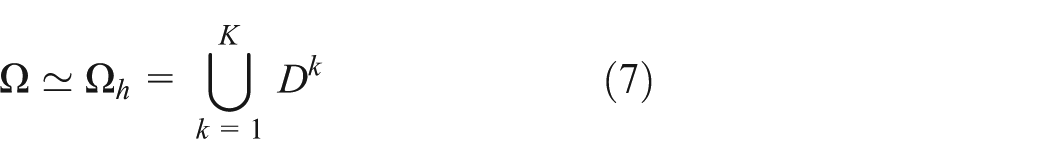
We consider straight-sided triangles although other options are possible. For example, in the case of a domain with curved boundary, elements of higher order can improve accuracy by describing the boundary more accurately (cf. Krivodonova and Berger
14
and Toulorge and Desmet
15
). Within each triangle
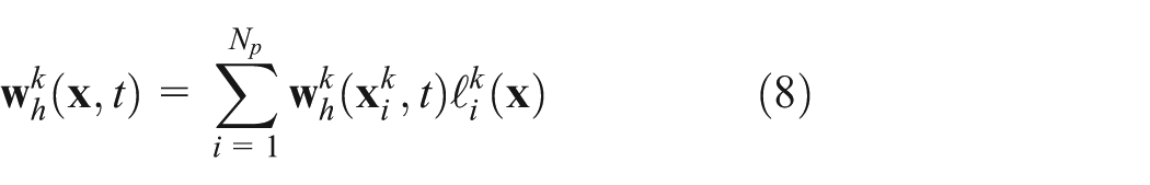
where

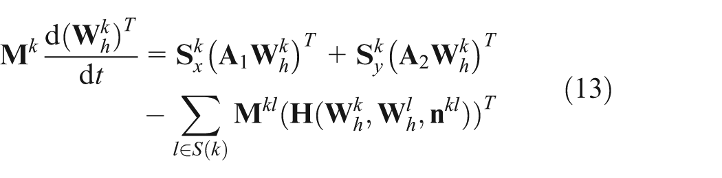
Local solutions

Applying Gauss’s divergence theorem, we obtain

where

where

where

and
where

and
The advantage of straight-sided triangles is that we can map each triangle to a reference triangle by means of linear transformation with a constant Jacobian matrix. This way, the above integrals need to be evaluated only once. We refer the reader to Hesthaven and Warburton 12 for more information on how to compute the matrices defined above efficiently.
Time discretization
As for time discretization, we used the explicit Runge–Kutta method of order 4. We shall focus on low-storage schemes due to memory requirements. Generally speaking, we want to solve an initial value problem for the system of ordinary differential equations of order 1, written in matrix form as

The low-storage explicit Runge–Kutta method reads as


where
Effect of the mesh
This section is devoted to studying the effect of the underlying mesh on the convergence rate of the numerical method presented in the previous section. The ideal theoretical convergence rate is
Our first step for applying the DGM to acoustic simulations was to test this method for solving the advection equation

for
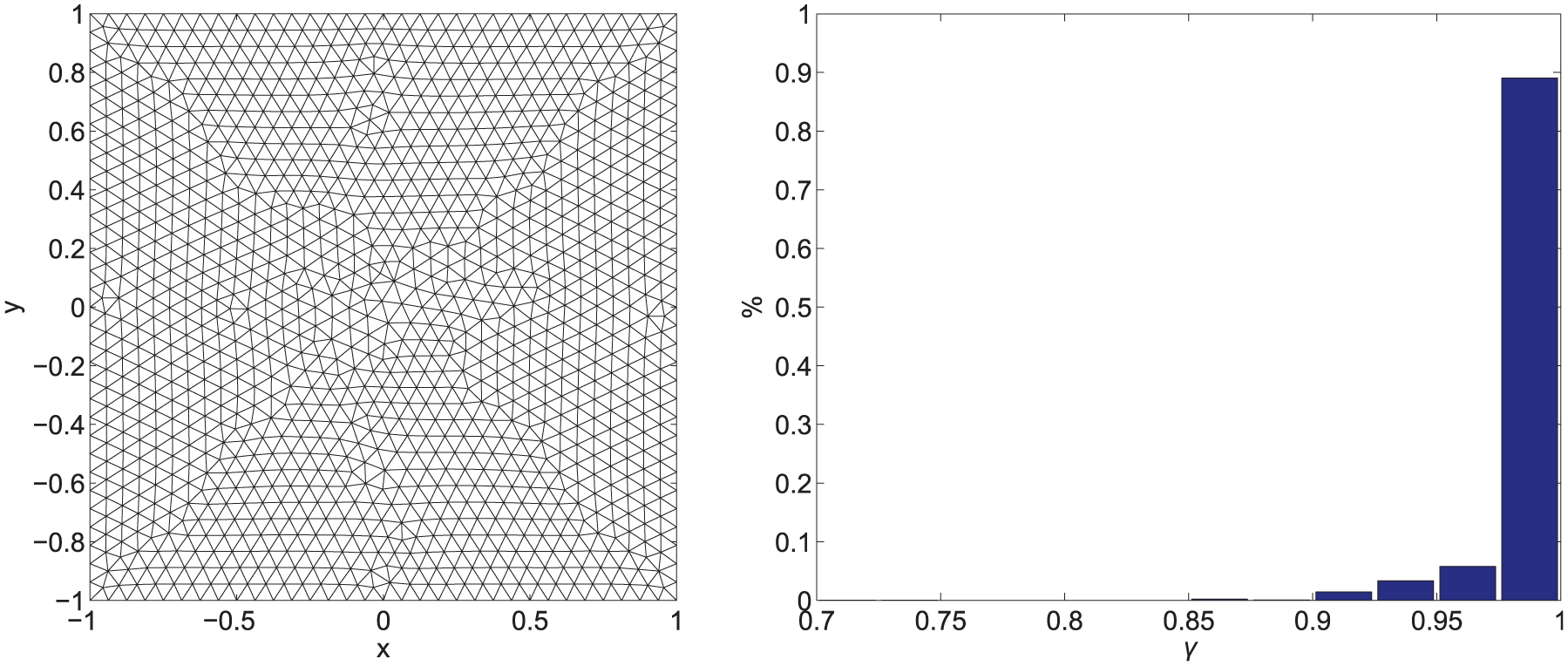
When talking about mesh quality, we have to define the shape quality parameter for an element. We used the one from Geuzaine and Remacle, 19 defined as

where

Gmsh mesh generator (Delaunay algorithm) – mesh (left) and quality parameter histogram (right).

Gmsh mesh generator (Frontal algorithm) – mesh (left) and quality parameter histogram (right).
Gambit mesh generator – mesh (left) and quality parameter histogram (right).
Based on our results, we can state that Gambit produces meshes of the highest quality. For a very fine mesh, we can see that Gambit produces mesh with the highest percentage of high-quality elements. We also observed that the Frontal algorithm produces a fairly structured mesh with most of the elements oriented in the same way. In contrast to that, the Delaunay algorithm implemented in Gmsh produces totally unstructured grids while element size varies more significantly.
When studying the convergence rate of the numerical method applied to the advection equation mentioned above, the following convergence rates were experimentally observed for the case
Convergence rates for different algorithms.

BCs
Next, we describe acoustic BCs. Reflecting BCs are used to reflect acoustic waves from the rigid wall in examples presented in subsections ‘Verification of reflecting BC’ and ‘Duct acoustics’. NRBCs are used to truncate the computational domain for the simulations corresponding to the sound propagation in an unbounded domain.
The reflecting BC is modelled by the slip condition, which is prescribed for the unknown perturbations (cf. Toulorge
20
). Let us denote

where

where

and

As for the NRBC, there are many possibilities to implement it. It can be modelled using characteristics (cf. Thomson 21 ) or various absorbing zones (cf. Mani 22 ). An overview can be found in Colonius, 23 Hu 24 and Richards et al. 25 In general, absorbing zones are designed in such a way that the waves are attenuated, yielding as little reflections as possible. We chose the PML approach and utilized the formulation from Hu. 7 Denoting
The modified LEE for uniform mean flow aligned with x-axis and with

where
and the right-hand side term is given by

Here,
Coefficients

where
To terminate the PML, we impose the following BCs, which were proposed in Hu. 7 These are

where

PML domain – absorption coefficients.
Discretization of equation (16) is carried out similarly to the LEE because these two sets of equations are formally similar. Furthermore, it was discovered that eigenvalues of the matrix
Acoustic simulations
In this section, we test the DGM on several benchmark problems of acoustics. The benchmark problems presented in this article are taken from the Proceedings of Computational Aeroacoustics Workshop sponsored by the National Aeronautics and Space Administration (NASA) and the Institute for Computer Applications in Science and Engineering (ICASE), published in 1995 as ICASE/LaRC Workshop on Benchmark Problems in Computational Aeroacoustics (cf. Tam 26 ). Our implementation in MATLAB environment was used to solve these test problems (based on DGM implementation presented in Hesthaven and Warburton 12 ).
For these test problems, we define the reference speed of sound,
It is convenient to use length, time, and density scales to further define velocity and pressure scales. We may then use a dimensionless version of LEE using these scales (cf. Tam
26
). The velocity of the mean flow is then specified by
Propagation of an acoustic pulse
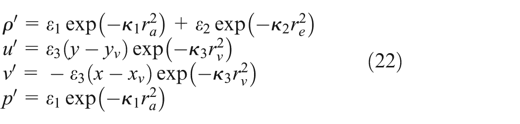
We begin with an initial value problem designed to simulate the propagation of acoustic waves. We consider a medium at rest, that is,

where
The analytical solution was derived in Tam and Webb.
11
We used it to evaluate the error of the numerical method. We considered a finite domain

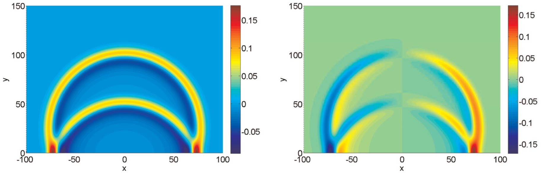
Solution for pressure perturbations – top view (left) and cut at

Solution for velocity perturbations
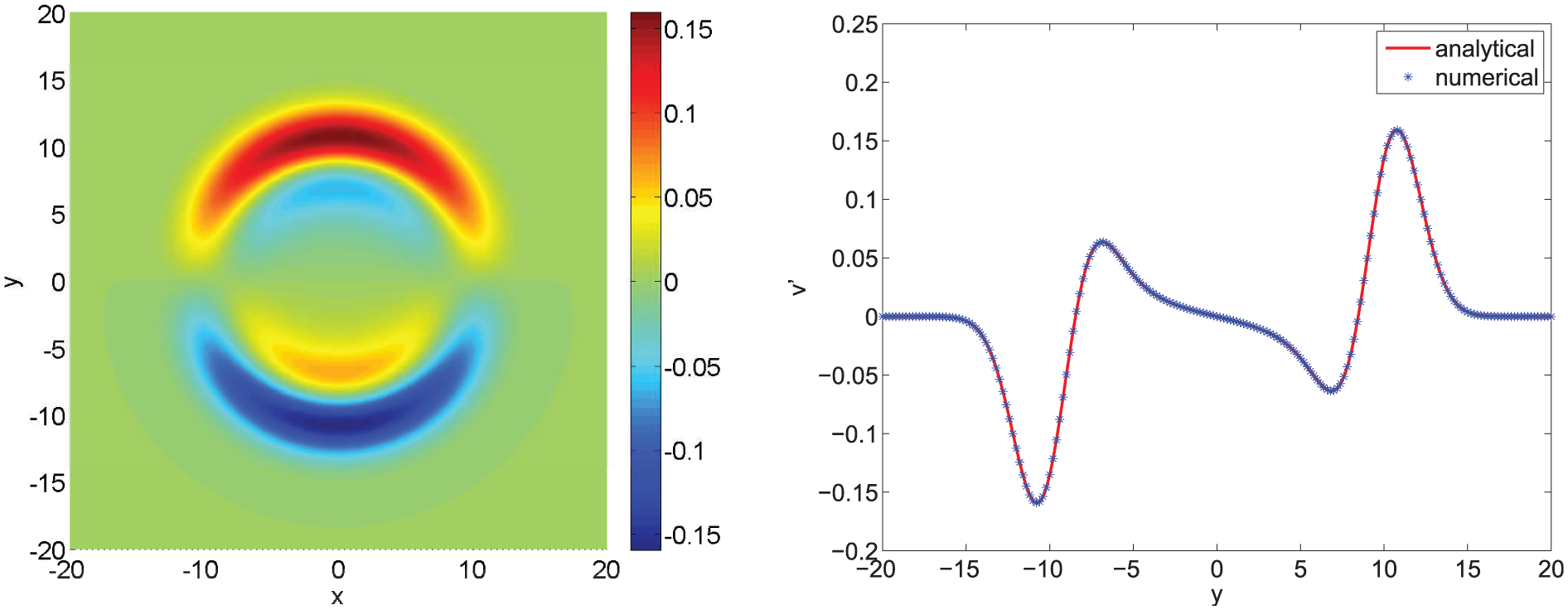
Solution for velocity perturbations
Seeing that the DGM is able to reproduce propagating acoustic waves very accurately, we would like to verify the convergence rate of this method. To this end, we solved this problem for different combinations of mesh size parameter

Specification of meshes.

The observed errors are plotted in Figure 8. The scale of both axes is set to be logarithmic and a line is fitted to these values in terms of the least squares method. The obtained convergence rates are presented in Table 4.
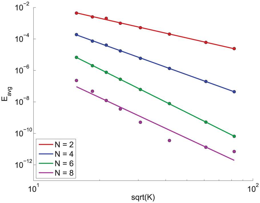
Convergence analysis for acoustic pulse propagation problem.
Convergence rates for acoustic pulse propagation.
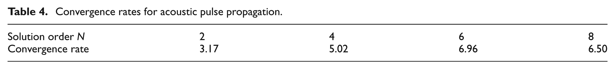
We can see that almost optimal convergence rates are obtained in all cases except for
Verification of reflecting BC
This is an initial value boundary problem to test the implemented reflecting BC. We again consider a medium at rest, that is,

where this
The analytical solution, presented in Tam,
26
was used to evaluate the numerical results. This time, our computational domain was

Domain and initial conditions.
We solved this problem using an element size parameter
Solution for density (left) and velocity

Solution for velocity
To show more clearly that the implemented reflecting BC yields satisfactory results, we present the solution for pressure perturbations along y-axis (on the left side) and pressure perturbations in time at point

Pressure fluctuations – cut at
Verification of NRBCs
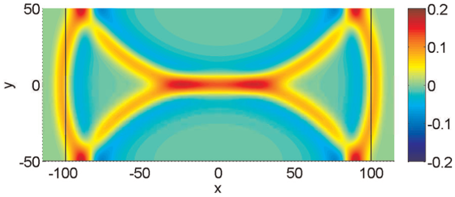
This is an initial value boundary problem designed to test the implemented NRBCs. The mean flow is assumed to be in the direction of the x-axis with its velocity equal to half of the reference speed of sound, that is,
where
Parameters

We compared our results with the analytical solution provided in Tam.
26
We assumed a computational domain
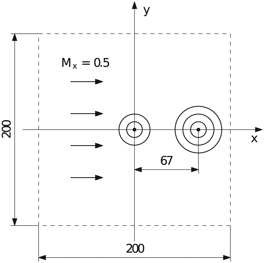
Domain and initial conditions.
We chose

Density (left) and velocity

Velocity
Duct acoustics
Duct acoustics is an important part of acoustic widely used in industry. Flow is often in one direction and the computational domain is bounded by walls in the other directions. The problem we now present does not have a known analytical solution. To verify the implemented NRBCs, we solved the same problem using a significantly larger computational domain terminated by reflecting BC on both ends. The secondary domain was chosen large enough so that the reflected waves are not able to reach our domain of interest. The solution obtained by simulation using the larger domain, truncated to the original computational domain, can then be used as a reference solution to the one obtained by simulation using the original domain with NRBCs.
Here, we attempt to solve a simple testing problem presented in Hu.
24
We assumed a uniform mean flow with

where
Our computational domain was a rectangular domain

Domain and initial condition.
We solved this problem using the element size parameter

Pressure fluctuations at
Pressure fluctuations at

Pressure fluctuations at

Pressure fluctuations at
Figure 21 shows the comparison with the solution obtained using domain

Comparison for pressure perturbations with reference solution in time at point
We see that all outgoing waves are correctly attenuated in the PML zones (compared to the reference solution obtained by the previous simulation on larger computational domain). These results are in agreement with those presented in Hu 24 and Nogueira et al. 29
Conclusion
We presented the nodal DGM as a suitable method for acoustic simulations. We performed simulations of acoustic pulse propagation to demonstrate that the DGM can reach a high convergence rate. We also tested typical acoustic BC, namely, reflecting BC and NRBC, and we verified that the DGM enables their effective implementation. In particular, we have also shown how to use the PML approach in the DGM. In addition, we demonstrated the importance of high-quality computational mesh. Our experiments revealed that the actual convergence rate of the method is strongly affected by quality of the underlying mesh.
All the experiments were done using MATLAB code. The algorithm was then ported to C++ programming language, which yielded approximately 3× shorter execution times. Additionally, work has begun on implementation of distributed simulation for computational cluster. We would like to extend the algorithm to 3D.
Footnotes
Academic Editor: Yi Wang
Declaration of conflicting interests
The author(s) declared no potential conflicts of interest with respect to the research, authorship and/or publication of this article.
Funding
The author(s) disclosed receipt of the following financial support for the research, authorship and/or publication of this article: This study was financially supported by the project no. GA 13-27505S, funded by the Czech Grant Agency.