Towards a combined perfectly matching layer and infinite element formulation for unbounded elastic wave problems

Abstract

This paper presents a framework for implementing a novel perfectly matching layer and infinite element (PML+IE) combination boundary condition for unbounded elastic wave problems in the time domain. To achieve this, traditional hexahedral finite elements are used to model wave propagation in the inner domain and IE test functions are implemented in the exterior domain. Two alternative implementations of the PML formulation are studied: the case with constant stretching in all three dimensions and the case with spatially dependent stretching along a single direction. The absorbing ability of the PML+IE formulation is demonstrated by the favourable comparison with the reflection coefficient for a plane wave incident on the boundary achieved using a finite-element-only approach where stress free boundary conditions are implemented at the domain edge. Values for the PML stretching function parameters are selected based on the minimisation of the reflected wave amplitude and it is shown that the same reduction in reflection amplitude can be achieved using the PML+IE approach with approximately half of the number of elements required in the finite-element-only approach.

1. Introduction

In numerical modelling and simulation, where resources are limited by memory and processing power [1], it is useful to study a small spatial domain containing the region of interest and simply assume that the outer domain extends to infinity [2]; for example, in aerospace problems, the infinite domain could be atmospheric air while the region of interest relates only to the localised flow around an airplane wing [3]. In cases such as this, it is necessary to employ a boundary condition on the exterior of the computational domain to prevent outgoing waves reflecting back into the region of interest. A number of methods exist to deal with these reflections within numerical simulations such as absorbing boundary conditions (ABCs) [4], perfectly matching layers (PMLs) [5] and infinite elements (IEs) [6]. A review of the use of such boundary conditions within the finite element method (FEM) for time-harmonic acoustics is carried out in [7–11].

The PML technique (first presented by Berenger [5]) is based on the use of an absorbing layer, with the matching medium designed to absorb without reflection and prevent any wave travelling back into the computational domain. While Berenger dealt with electromagnetic waves, Chew and Liu [12] proved that there exists a fictitious elastic PML half-space in solids which completely absorbs elastic waves in spite of the coupling between compressional and shear wave modes. In the same year, Lyons et al. [13] demonstrated the accuracy and potential of the PML in a finite element (FE) formulation. The work of Liu and Tao [14] and Qi and Geers [15] extended the PML to simulate acoustic wave propagation in absorptive media. The PML was also shown to be effective in numerically solving the Helmholtz equation in [16, 17] and was developed further for time harmonic elastodynamics in [18, 19]. Methods for modelling the elastic wave equation with PMLs in both the time and frequency domain are examined in [20–26]. Examination of PMLs in the specific case of a forced, open, elastic waveguide has been carried out in [25], where PMLs were implemented in the radial direction (the direction orthogonal to the wave propagation direction) along the length of the waveguide to model a buried bar. The modal analysis that this allowed investigated the roll of this radial PML on the wavenumber spectrum, the attenuation as a function of frequency, and the form of the mode shapes.

An alternative approach to truncating the FE mesh is to employ IEs at the boundary. These IEs essentially extend the element domain to infinity, and are based on the shape functions used in the interior elements which are multiplied by an appropriate decay function to achieve the desired behaviour at infinity. The IE method was discussed in detail by Bettess [6] while Astley provides a review of IE formulations with various element types and assesses their accuracy in [27]. IEs have been applied to the acoustic wave equation in the frequency domain [28–32] and in the time domain [33–35], as well as to the elastic wave equation [36, 37]. Transient IEs have also been explored [38, 39].

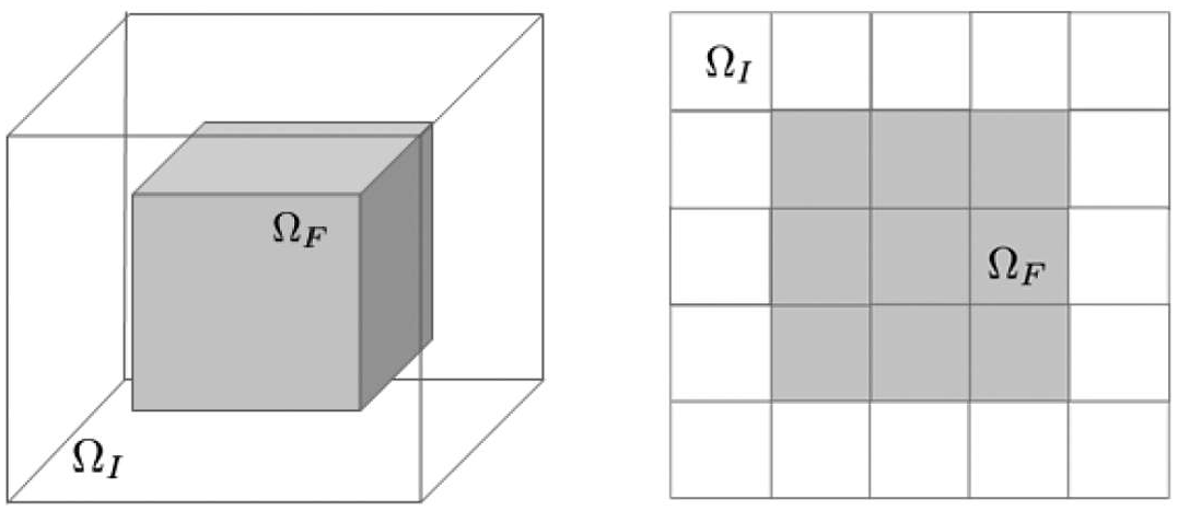
Building on this existing body of work, the authors developed a combined PML+IE method for unbounded acoustic problems in the frequency domain and assessed its performance for a spherical resonator [40]. This approach was extended in [41] to consider the scalar wave equation in the time domain. In the present paper, a method for studying elastodynamic waves in a three-dimensional, homogeneous volume with the PML+IE formulation implemented at the boundary (see Figure 1) is presented. This work is believed to be the first FE implementation of a combined PML+IE formulation for the vector elastic wave equation in the time domain. A numerical study of a three-dimensional, homogeneous volume placed in a vacuum with PML+IE boundary conditions applied at the right-most face of the domain (the face $x_1=L_1$ shown in Figure 2) is conducted, allowing an empirical comparison of the method to a FE-only approach where stress free boundary conditions are employed at this boundary. In contrast to the elastodynamic wave problem considered in [25], which is developed specifically for waveguides where Dirichlet boundary conditions are implemented on the outer edge of the PML domain and the system is solved using an implicit scheme, in this paper the focus is on examining the time-domain reflection coefficient from the end of a three-dimensional volume in the direction of wave propagation, owing to the PML+IE formulation. Here, an IE formulation is implemented in conjunction with the PML at the open end of the three-dimensional volume and standard stress-free boundary conditions are applied along its length. In addition, this paper opts for an explicit FE formulation, choosing to compromise some numerical accuracy in return for increased computational efficiency. This will facilitate the use of the method in three-dimensional problems with PML+IE boundary conditions at all domain boundaries.

Figure 1.

In the general, three-dimensional formulation, the domain of interest ${\mathrm{\Omega }}_F$ is modelled by standard FEs (shaded here) and bordered in all directions by elements modelled using PML+IE combinations; this domain is denoted ${\mathrm{\Omega }}_I$ . The schematic on the right represents a cross-section in any plane of the three-dimensional case.

Figure 2.

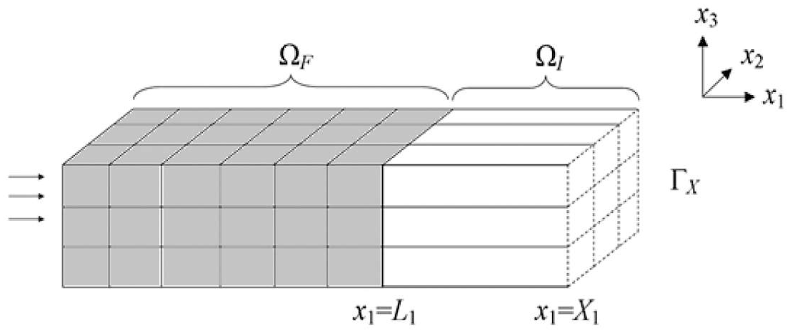
A homogeneous rectangular elastic volume with an open end operating in a vacuum where the arrows depict excitation of the left-most elements by some time-limited function. The interior domain ${\mathrm{\Omega }}_F$ is of fixed length $L_1$ and is meshed using standard FEs, depicted here by the shaded region. The exterior domain ${\mathrm{\Omega }}_I$ is implemented at the right end of the three-dimensional volume (the open, semi-infinite part of the domain) and uses the PML+IE combination. The face ${\mathrm{\Gamma }}_X$ at $x_1=X_1$ is a notional face that will later be allowed to tend to infinity.

We begin with the elastodynamic wave equation and a Fourier transform in time is taken in order to introduce appropriate coordinate stretching transformations. The variational formulation is used to introduce IEs under the assumption that the material is locally isotropic. The problem is then discretised with traditional hexahedral FEs modelling the inner domain and IE test functions employed in the exterior domain. Two scenarios are considered: the case with constant PML stretching in all three directions and the case with spatially dependent stretching in one direction. To arrive at an explicit time-domain formulation, diagonalisation of the velocity coefficient matrix is implemented. A reflection coefficient is defined and used to compare the new PML+IE formulation with an extended FE-domain-only implementation (where stress-free boundary conditions are implemented in place of the PML+IE formulation). Values for the PML stretching function parameters are then selected based on the minimisation of the reflected wave amplitude and it is shown that to achieve the same reduction in reflected wave amplitude as observed in the PML+IE case, twice the number of elements (and, thus, twice the runtime) is required in the FE-only implementation.

2. Geometry and governing equations

Consider the problem of an open-ended, homogeneous, three-dimensional volume with the geometry shown in Figure 2, where ${\mathrm{\Gamma }}_X$ is a notional face at $x_1=X_1$ which will later be allowed to tend to infinity, ${\mathrm{\Omega }}_F$ is the inner domain, modelled by conventional FEM techniques, and ${\mathrm{\Omega }}_I$ is the outer domain, modelled by PML and IE combinations. The elements which lie on the left-hand boundary of the domain are excited by some time-limited input function (depicted by the arrows in Figure 2). The governing elastodynamic equations are [42]

$$\rho \frac{\partial v_i}{\partial t}=\sum _{j=1}^3\frac{\partial {\sigma }_{\mathrm{ij}}}{\partial x_j},$$

(1)

where $\rho$ is density, $v$ is velocity, ${\sigma }_{\mathrm{ij}}$ denotes the stress tensor and

$$\frac{\partial {\sigma }_{\mathrm{ij}}}{\partial t}=\sum _{k,l=1}^3{C}_{\mathrm{ijkl}}\frac{\partial v_k}{\partial x_l},$$

(2)

with $C_{\mathrm{ijkl}}$ the stiffness tensor. We now define a transformation

$$\frac{\partial }{\partial {\tilde{x}}_j}=\frac{1}{s_j}\frac{\partial }{\partial x_j}$$

(3)

where

$$s_j(x_j,\omega )=\{\begin{array}{cc}1\hfill & \mathrm{in}{\mathrm{\Omega }}_F\hfill \\ \multicolumn{1}{c}{{\alpha }_j(x_j)(1+\frac{i}{\omega }{\beta }_j(x_j))}& \mathrm{in}{\mathrm{\Omega }}_I.\hfill \end{array}$$

(4)

Here ${\alpha }_j,{\beta }_j$ are functions which can be used to fine tune the stretching function and $\omega$ is the angular frequency. By writing (1) and (2) in terms of the stretched coordinates ${\tilde{x}}_j$ (assuming $v_i(\mathbf{x},0)=0$ and ${\sigma }_{\mathrm{ij}}(\mathbf{x},0)=0$ ), and taking a Fourier transform in time we can write

$$-i\omega \rho {\hat{v}}_i=\sum _{j=1}^3\frac{1}{s_j}\frac{\partial {\hat{\sigma }}_{\mathrm{ij}}}{\partial x_j},$$

(5)

$$-i\omega {\hat{\sigma }}_{\mathrm{ij}}=\sum _{k,l=1}^3\frac{C_{\mathrm{ijkl}}}{s_l}\frac{\partial {\hat{v}}_k}{\partial x_l}.$$

(6)

Stress-free boundary conditions are implemented on all faces except ${\mathrm{\Gamma }}_X$ where the Sommerfeld radiation condition

$$\nabla {\hat{v}}_i=-\mathrm{ik}{\hat{v}}_i+ϵ\mathrm{on}{\mathrm{\Gamma }}_X,$$

(7)

is employed, where $ϵ=O(1/X_1^2)$ and $k=\omega /c$ is the wavenumber (here $c$ can be chosen as either the wave speed of a compressional or shear wave). Thus, by multiplying both sides of (5) by a test function $w$ , integrating over the whole domain $\mathrm{\Omega }={\mathrm{\Omega }}_F\cup {\mathrm{\Omega }}_I$ and applying the divergence theorem, we can eventually write

$${\int }_{\mathrm{\Omega }}-i\omega \rho {\hat{v}}_{i}w\mathrm{d}\mathrm{\Omega }={\int }_{{\mathrm{\Gamma }}_X}\sum _{j,k,l=1}^3\frac{C_{\mathrm{ijkl}}}{s_j{s}_l}(\frac{1}{c}{\hat{v}}_k+\frac{ϵ}{-i\omega })w\mathrm{d}{\mathrm{\Gamma }}_X-{\int }_{\mathrm{\Omega }}\sum _{j=1}^3\frac{1}{s_j}{\hat{\sigma }}_{\mathrm{ij}}\frac{\partial w}{\partial x_j}\mathrm{d}\mathrm{\Omega }.$$

(8)

Note, to examine the case of a clamped domain (that is, where zero velocity boundary conditions are applied along the length of the domain), we would instead multiply (6) by our test function $w$ , integrate and apply the divergence theorem. This would provide a different start point for the forthcoming analysis and so is beyond the scope of this paper, but would make for an interesting extension in future studies.

To discretise equation (8), we let $\hat{\mathbf{v}}=(\hat{p},\hat{q},\hat{r})$ , where $\hat{p}={\sum }_{j=1}^N{\varphi }_j(x_1,x_2,x_3){\hat{p}}_j(\omega )$ , $\hat{q}={\sum }_{j=1}^N{\varphi }_j(x_1,$ $x_2,x_3){\hat{q}}_j(\omega )$ and $\hat{r}={\sum }_{j=1}^N{\varphi }_j(x_1,x_2,x_3){\hat{r}}_j(\omega )$ . Switching to Voigt notation, we also write ${\hat{\sigma }}_i={\sum }_{j=1}^N{\varphi }_j(x_1,x_2,x_3){\hat{\gamma }}_{\mathrm{ij}}(\omega )$ . Note that in these expressions, subscript $j$ refers to the node in the FE discretisation and ${\varphi }_j$ denotes the basis functions given by

$${\varphi }_j(x_1,x_2,x_3)=\{\begin{array}{cc}{N}_j(x_1,x_2,x_3)\hfill & \mathrm{in}{\mathrm{\Omega }}_F\hfill \\ \multicolumn{1}{c}{f_j(x_1,\omega )g_j(x_2,x_3)}& \mathrm{in}{\mathrm{\Omega }}_I\hfill \end{array}(j=1,\dots ,N).$$

(9)

The test function $w$ is also replaced by a series of test functions ${\theta }_i$ of compact support given by

$${\theta }_i(x_1,x_2,x_3)=\{\begin{array}{cc}{N}_i(x_1,x_2,x_3)\hfill & \mathrm{in}{\mathrm{\Omega }}_F\hfill \\ \multicolumn{1}{c}{w_i(x_1,\omega )g_i(x_2,x_3)}& \mathrm{in}{\mathrm{\Omega }}_I\hfill \end{array}(i=1,\dots ,N).$$

(10)

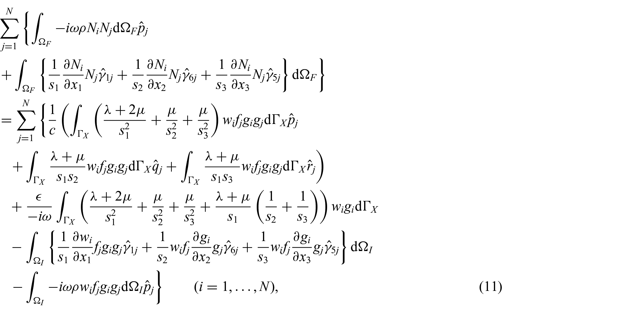
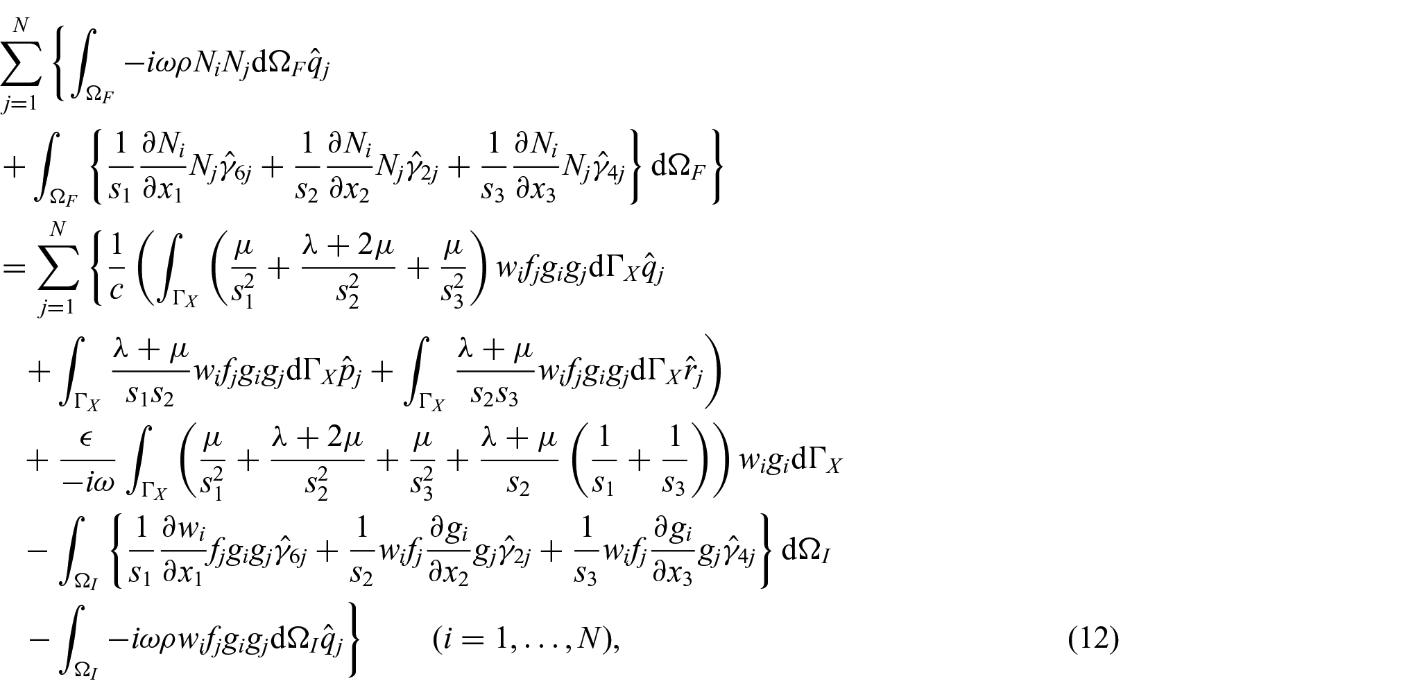
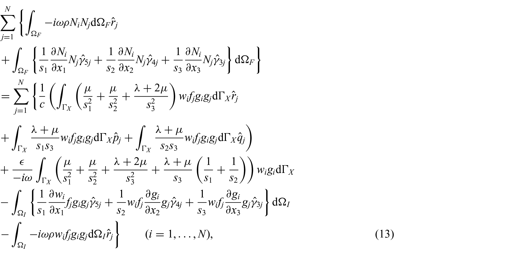
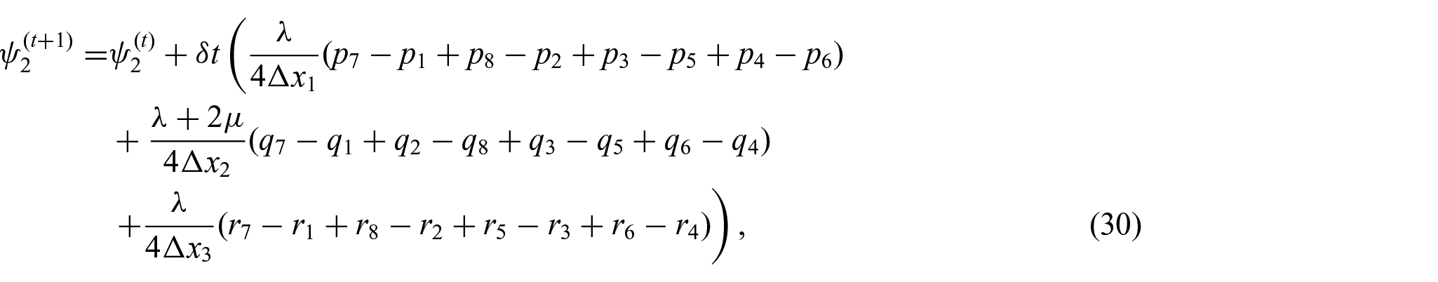
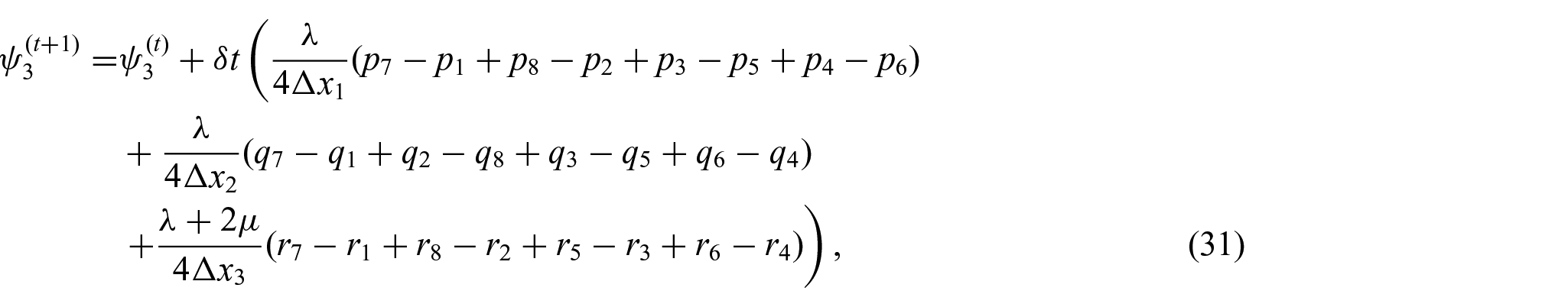
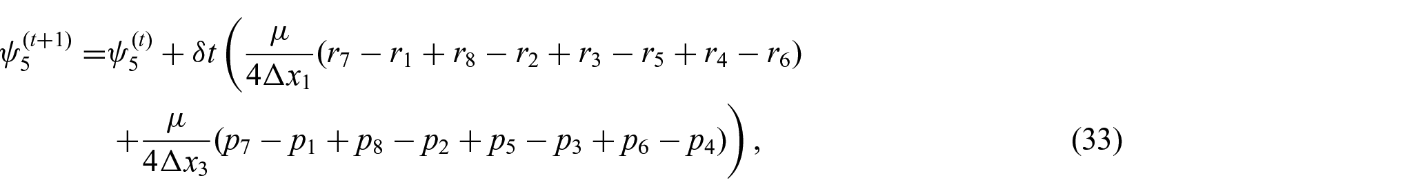
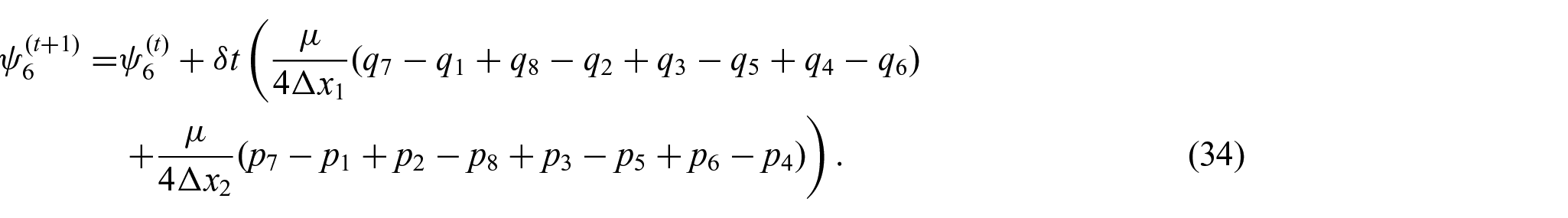
The functional form of such basis functions will be given in the following sections. Assuming an isotropic stiffness tensor, equation (8) gives rise to the equations

$$\begin{array}{c}\sum _{j=1}^N\{{\int }_{{\mathrm{\Omega }}_F}-i\omega \rho N_i{N}_j\mathrm{d}{\mathrm{\Omega }}_F{\hat{p}}_j\hfill \\ +{\int }_{{\mathrm{\Omega }}_F}\{\frac{1}{s_1}\frac{\partial N_i}{\partial x_1}{N}_j{\hat{\gamma }}_{1j}+\frac{1}{s_2}\frac{\partial N_i}{\partial x_2}{N}_j{\hat{\gamma }}_{6j}+\frac{1}{s_3}\frac{\partial N_i}{\partial x_3}{N}_j{\hat{\gamma }}_{5j}\}\mathrm{d}{\mathrm{\Omega }}_F\}\hfill \\ =\sum _{j=1}^N\{\frac{1}{c}({\int }_{{\mathrm{\Gamma }}_X}(\frac{\lambda +2\mu }{s_1^2}+\frac{\mu }{s_2^2}+\frac{\mu }{s_3^2})w_i{f}_j{g}_i{g}_j\mathrm{d}{\mathrm{\Gamma }}_X{\hat{p}}_j\hfill \\ +{\int }_{{\mathrm{\Gamma }}_X}\frac{\lambda +\mu }{s_1{s}_2}{w}_i{f}_j{g}_i{g}_j\mathrm{d}{\mathrm{\Gamma }}_X{\hat{q}}_j+{\int }_{{\mathrm{\Gamma }}_X}\frac{\lambda +\mu }{s_1{s}_3}{w}_i{f}_j{g}_i{g}_j\mathrm{d}{\mathrm{\Gamma }}_X{\hat{r}}_j)\hfill \\ +\frac{ϵ}{-i\omega }{\int }_{{\mathrm{\Gamma }}_X}(\frac{\lambda +2\mu }{s_1^2}+\frac{\mu }{s_2^2}+\frac{\mu }{s_3^2}+\frac{\lambda +\mu }{s_1}(\frac{1}{s_2}+\frac{1}{s_3}))w_i{g}_i\mathrm{d}{\mathrm{\Gamma }}_X\hfill \\ -{\int }_{{\mathrm{\Omega }}_I}\{\frac{1}{s_1}\frac{\partial w_i}{\partial x_1}{f}_j{g}_i{g}_j{\hat{\gamma }}_{1j}+\frac{1}{s_2}{w}_i{f}_j\frac{\partial g_i}{\partial x_2}{g}_j{\hat{\gamma }}_{6j}+\frac{1}{s_3}{w}_i{f}_j\frac{\partial g_i}{\partial x_3}{g}_j{\hat{\gamma }}_{5j}\}\mathrm{d}{\mathrm{\Omega }}_I\hfill \\ -{\int }_{{\mathrm{\Omega }}_I}-i\omega \rho w_i{f}_j{g}_i{g}_j\mathrm{d}{\mathrm{\Omega }}_I{\hat{p}}_j\}(i=1,\dots ,N),\hfill \end{array}$$

(11)

$$\begin{array}{c}\sum _{j=1}^N\{{\int }_{{\mathrm{\Omega }}_F}-i\omega \rho N_i{N}_j\mathrm{d}{\mathrm{\Omega }}_F{\hat{q}}_j\hfill \\ +{\int }_{{\mathrm{\Omega }}_F}\{\frac{1}{s_1}\frac{\partial N_i}{\partial x_1}{N}_j{\hat{\gamma }}_{6j}+\frac{1}{s_2}\frac{\partial N_i}{\partial x_2}{N}_j{\hat{\gamma }}_{2j}+\frac{1}{s_3}\frac{\partial N_i}{\partial x_3}{N}_j{\hat{\gamma }}_{4j}\}\mathrm{d}{\mathrm{\Omega }}_F\}\hfill \\ =\sum _{j=1}^N\{\frac{1}{c}({\int }_{{\mathrm{\Gamma }}_X}(\frac{\mu }{s_1^2}+\frac{\lambda +2\mu }{s_2^2}+\frac{\mu }{s_3^2})w_i{f}_j{g}_i{g}_j\mathrm{d}{\mathrm{\Gamma }}_X{\hat{q}}_j\hfill \\ +{\int }_{{\mathrm{\Gamma }}_X}\frac{\lambda +\mu }{s_1{s}_2}{w}_i{f}_j{g}_i{g}_j\mathrm{d}{\mathrm{\Gamma }}_X{\hat{p}}_j+{\int }_{{\mathrm{\Gamma }}_X}\frac{\lambda +\mu }{s_2{s}_3}{w}_i{f}_j{g}_i{g}_j\mathrm{d}{\mathrm{\Gamma }}_X{\hat{r}}_j)\hfill \\ +\frac{ϵ}{-i\omega }{\int }_{{\mathrm{\Gamma }}_X}(\frac{\mu }{s_1^2}+\frac{\lambda +2\mu }{s_2^2}+\frac{\mu }{s_3^2}+\frac{\lambda +\mu }{s_2}(\frac{1}{s_1}+\frac{1}{s_3}))w_i{g}_i\mathrm{d}{\mathrm{\Gamma }}_X\hfill \\ -{\int }_{{\mathrm{\Omega }}_I}\{\frac{1}{s_1}\frac{\partial w_i}{\partial x_1}{f}_j{g}_i{g}_j{\hat{\gamma }}_{6j}+\frac{1}{s_2}{w}_i{f}_j\frac{\partial g_i}{\partial x_2}{g}_j{\hat{\gamma }}_{2j}+\frac{1}{s_3}{w}_i{f}_j\frac{\partial g_i}{\partial x_3}{g}_j{\hat{\gamma }}_{4j}\}\mathrm{d}{\mathrm{\Omega }}_I\hfill \\ -{\int }_{{\mathrm{\Omega }}_I}-i\omega \rho w_i{f}_j{g}_i{g}_j\mathrm{d}{\mathrm{\Omega }}_I{\hat{q}}_j\}(i=1,\dots ,N),\hfill \end{array}$$

(12)

and

$$\begin{array}{c}\sum _{j=1}^N\{{\int }_{{\mathrm{\Omega }}_F}-i\omega \rho N_i{N}_j\mathrm{d}{\mathrm{\Omega }}_F{\hat{r}}_j\hfill \\ +{\int }_{{\mathrm{\Omega }}_F}\{\frac{1}{s_1}\frac{\partial N_i}{\partial x_1}{N}_j{\hat{\gamma }}_{5j}+\frac{1}{s_2}\frac{\partial N_i}{\partial x_2}{N}_j{\hat{\gamma }}_{4j}+\frac{1}{s_3}\frac{\partial N_i}{\partial x_3}{N}_j{\hat{\gamma }}_{3j}\}\mathrm{d}{\mathrm{\Omega }}_F\}\hfill \\ =\sum _{j=1}^N\{\frac{1}{c}({\int }_{{\mathrm{\Gamma }}_X}(\frac{\mu }{s_1^2}+\frac{\mu }{s_2^2}+\frac{\lambda +2\mu }{s_3^2})w_i{f}_j{g}_i{g}_j\mathrm{d}{\mathrm{\Gamma }}_X{\hat{r}}_j\hfill \\ +{\int }_{{\mathrm{\Gamma }}_X}\frac{\lambda +\mu }{s_1{s}_3}{w}_i{f}_j{g}_i{g}_j\mathrm{d}{\mathrm{\Gamma }}_X{\hat{p}}_j+{\int }_{{\mathrm{\Gamma }}_X}\frac{\lambda +\mu }{s_2{s}_3}{w}_i{f}_j{g}_i{g}_j\mathrm{d}{\mathrm{\Gamma }}_X{\hat{q}}_j)\hfill \\ +\frac{ϵ}{-i\omega }{\int }_{{\mathrm{\Gamma }}_X}(\frac{\mu }{s_1^2}+\frac{\mu }{s_2^2}+\frac{\lambda +2\mu }{s_3^2}+\frac{\lambda +\mu }{s_3}(\frac{1}{s_1}+\frac{1}{s_2}))w_i{g}_i\mathrm{d}{\mathrm{\Gamma }}_X\hfill \\ -{\int }_{{\mathrm{\Omega }}_I}\{\frac{1}{s_1}\frac{\partial w_i}{\partial x_1}{f}_j{g}_i{g}_j{\hat{\gamma }}_{5j}+\frac{1}{s_2}{w}_i{f}_j\frac{\partial g_i}{\partial x_2}{g}_j{\hat{\gamma }}_{4j}+\frac{1}{s_3}{w}_i{f}_j\frac{\partial g_i}{\partial x_3}{g}_j{\hat{\gamma }}_{3j}\}\mathrm{d}{\mathrm{\Omega }}_I\hfill \\ -{\int }_{{\mathrm{\Omega }}_I}-i\omega \rho w_i{f}_j{g}_i{g}_j\mathrm{d}{\mathrm{\Omega }}_I{\hat{r}}_j\}(i=1,\dots ,N),\hfill \end{array}$$

(13)

where $\lambda$ and $\mu$ denote the Lamé constants.

In order to progress, some decisions must be made about the stretching function. Two scenarios will be considered: the first has constant stretching in all three directions, that is, $s_1=s_2=s_3\equiv s$ ; the second scenario has stretching in only one direction, retaining some spatial dependency, where $s_2=s_3\equiv 1$ and $s_1$ is a function of $x_1$ . Note, however, that in both cases $s$ is still a function of frequency.

3. Constant stretching

To simplify the integrals which appear in (11)–(13), we choose first to implement a constant stretching approach, where $s_j$ is independent of $x_j$ , that is, $s_1=s_2=s_3\equiv s$ . We define the basis functions as functions of a local coordinate system $(\xi ,\eta ,\zeta )$ centred on the node $j\prime$

$$N_{j^{\prime }}(\xi ,\eta ,\zeta )=\frac{1}{8}(1+\xi {\xi }_{j^{\prime }})(1+\eta {\eta }_{j^{\prime }})(1+\zeta {\zeta }_{j^{\prime }})\mathrm{in}{\mathrm{\Omega }}_F,$$

(14)

$$f_{j^{\prime }}(x_1,\omega )=\left(\frac{L_1}{x_1}\right)e^{-ik(x_1-L_1)}\mathrm{in}{\mathrm{\Omega }}_I,$$

(15)

$$g_{j^{\prime }}(\eta ,\zeta )=\frac{1}{4}(1+\eta {\eta }_{j^{\prime }})(1+\zeta {\zeta }_{j^{\prime }})\mathrm{in}{\mathrm{\Omega }}_I,$$

(16)

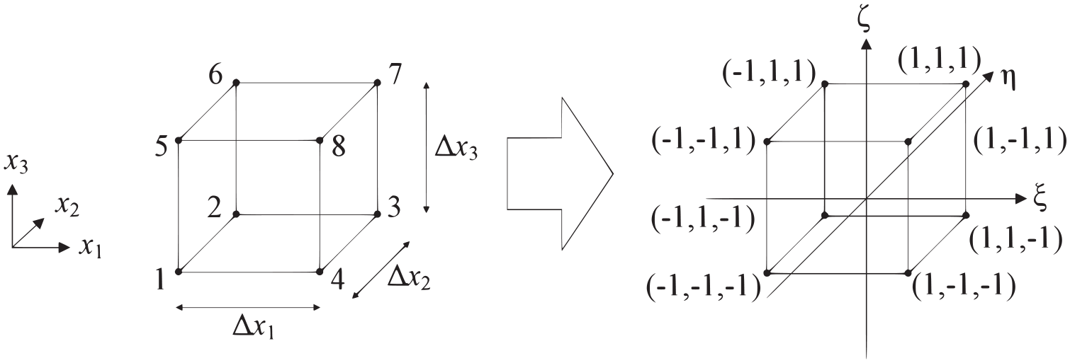
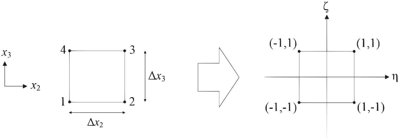
where $L_1$ is the fixed length of the interior domain. Next, a parameterisation in terms of these local coordinates of the FEs and IEs is introduced. In ${\mathrm{\Omega }}_I$ , this parameterisation is only used in the $x_2$ and $x_3$ directions. The mappings are shown in Figures 3 and 4 and the test functions are chosen as

$$N_{i^{\prime }}(\xi ,\eta ,\zeta )=\frac{1}{8}(1+\xi {\xi }_{i^{\prime }})(1+\eta {\eta }_{i^{\prime }})(1+\zeta {\zeta }_{i^{\prime }})\mathrm{in}{\mathrm{\Omega }}_F$$

(17)

$$w_{i^{\prime }}(x_1,\omega )={\left(\frac{L_1}{x_1}\right)}^3{e}^{ik(x_1-L_1)}\equiv {\left(\frac{L_1}{x_1}\right)}^2\mathrm{conj}\left\{f_{j^{\prime }}\right\}\mathrm{in}{\mathrm{\Omega }}_I,$$

(18)

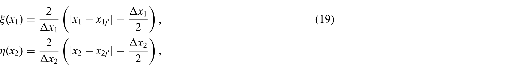
where the choice of $w_{i\prime }$ is based on the Astley–Leis IE [27]. Now with the mappings shown in Figure 3, we assume that instead

$$\begin{array}{c}\xi (x_1)=\frac{2}{\Delta x_1}(|x_1-x_{1j\prime }|-\frac{\Delta x_1}{2}),\\ \eta (x_2)=\frac{2}{\Delta x_2}(|x_2-x_{2j\prime }|-\frac{\Delta x_2}{2}),\end{array}$$

(19)

and

$$\zeta (x_3)=\frac{2}{\Delta x_3}(|x_3-x_{3j\prime }|-\frac{\Delta x_3}{2}),$$

where $\Delta x_i$ for $i=1,2,3$ denote the element sidelengths. Hence, the $N_{i\prime }$ basis functions have value $1$ at node $i\prime$ and value $0$ at all other nodes, and form a continuous function whose support is in the elements of which node $i\prime$ is a vertex.

Figure 3.

The mapping of the FEs (in ${\mathrm{\Omega }}_F$ ) in global coordinates $(x_1,x_2,x_3)$ to local coordinates $(\xi ,\eta ,\zeta )$ with node numbering indicated as shown. The local node numbering $i\prime =1,\dots ,8,$ is used in the schematic on the left.

Figure 4.

The mapping of the IEs (in ${\mathrm{\Omega }}_I$ ) in global coordinates $(x_2,x_3)$ to local coordinates $(\eta ,\zeta )$ with node numbering indicated as shown. The local node numbering $i\prime =1,\dots ,4,$ is used in the figure on the left and the $x_1$ direction (the IE direction) points out of the plane of the page.

It is also worth noting that, in this work, the assumption has been made that the stress components at a local node $i\prime$ , given by ${\hat{\gamma }}_{\mathrm{ni}\prime }$ for $n=1,\dots ,6$ , are equal to the stress components at local node $j\prime$ , given by ${\hat{\gamma }}_{\mathrm{nj}\prime }$ for $n=1,\dots ,6$ , when nodes $i\prime$ and $j\prime$ belong to the same element. Therefore, ${\hat{\gamma }}_{\mathrm{ni}\prime }={\hat{\gamma }}_{\mathrm{nj}\prime }\equiv {\hat{\psi }}_n$ for $i\prime ,j\prime \in {\mathrm{\Omega }}_e$ , where ${\mathrm{\Omega }}_e$ is either a FE or IE. Consequently, the stress component ${\hat{\gamma }}_{\mathrm{ni}\prime }$ at a local node $i\prime$ , is replaced by the stress component for the element under consideration, ${\hat{\psi }}_n$ .

Now, for computational speed, we want to derive an explicit scheme to solve the discretised elastodynamic equations. Currently, the discretised system of (11)–(13) lead to an implicit set of algebraic equations in the unknowns. Deriving an explicit scheme would require the inversion of a very large coefficient matrix which could only be conducted numerically, would be computationally expensive and demand increased memory requirements. An alternative approach is to approximate this matrix by a diagonal one whose inversion is trivial and, hence, facilitates the derivation of a computationally efficient explicit integration scheme. This approximation is made by summing the entries within each row of the velocity coefficient matrix and replacing the diagonal entry with this sum, setting all other entries to zero. This is predicated on the assumption that there are no sharp changes in the velocities and so adjacent nodes have very similar values and hence one can approximate the value at one node by the value at its neighbour. Specifically, in this constant stretching scenario, this approximation is subject to the conditions $\alpha >>\mu /\rho c^2$ and $\alpha >>(c_p/c_s{)}^2/4$ , where $c_s$ is the shear wave speed and $c_p$ is the longitudinal wave speed. Physically, from the first condition we observe that, if $c$ is set equal to the shear wave speed $c_s$ , then $\alpha >>1$ . This is in agreement with the second condition when $c_s\approx c_p/2$ , which is a typical ratio between the longitudinal and shear wave speeds in many engineering materials. Through the diagonalisation of the velocity coefficient matrix, a frequency domain approximation for each FE and IE can eventually be reached [43]. The left-hand side of (11)–(13) for each element then become (after taking inverse Fourier transforms)

$$\begin{array}{c}{A}_{1i\prime }^{(F)}=\frac{\rho \Delta x_1\Delta x_2\Delta x_3}{8}{\stackrel{·}{p}}_{i\prime }\hfill \\ +{\chi }_{i\prime }^{0,2}\frac{\Delta x_2\Delta x_3}{4}{\psi }_1+{\chi }_{i\prime }^{1,2}\frac{\Delta x_1\Delta x_3}{4}{\psi }_6+{\chi }_{i\prime }^{0,4}\frac{\Delta x_1\Delta x_2}{4}{\psi }_5(i\prime =1,\dots ,8),\hfill \end{array}$$

(20)

$$\begin{array}{c}{A}_{2i\prime }^{(F)}=\frac{\rho \Delta x_1\Delta x_2\Delta x_3}{8}{\stackrel{·}{q}}_{i\prime }\hfill \\ +{\chi }_{i\prime }^{0,2}\frac{\Delta x_2\Delta x_3}{4}{\psi }_6+{\chi }_{i\prime }^{1,2}\frac{\Delta x_1\Delta x_3}{4}{\psi }_2+{\chi }_{i\prime }^{0,4}\frac{\Delta x_1\Delta x_2}{4}{\psi }_4(i\prime =1,\dots ,8),\hfill \end{array}$$

(21)

and

$$\begin{array}{c}{A}_{3i\prime }^{(F)}=\frac{\rho \Delta x_1\Delta x_2\Delta x_3}{8}{\stackrel{·}{r}}_{i\prime }\hfill \\ +{\chi }_{i\prime }^{0,2}\frac{\Delta x_2\Delta x_3}{4}{\psi }_5+{\chi }_{i\prime }^{1,2}\frac{\Delta x_1\Delta x_3}{4}{\psi }_4+{\chi }_{i\prime }^{0,4}\frac{\Delta x_1\Delta x_2}{4}{\psi }_3(i\prime =1,\dots ,8),\hfill \end{array}$$

(22)

where

$${\chi }_{i\prime }^{m,n}=(-1{)}^{\phi }\mathrm{with}\phi =\lceil \frac{i\prime +m}{2n}\rceil ,$$

(23)

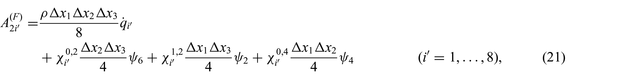
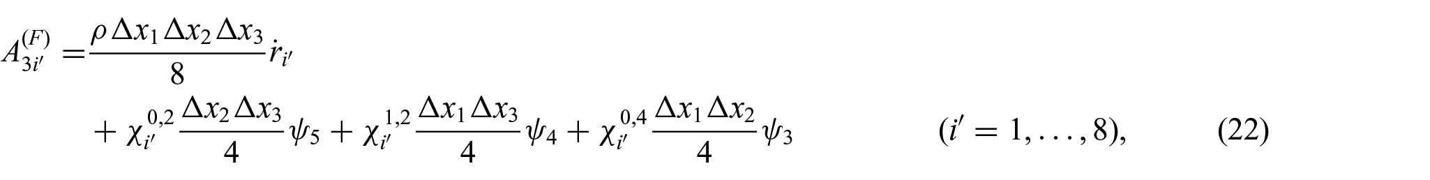
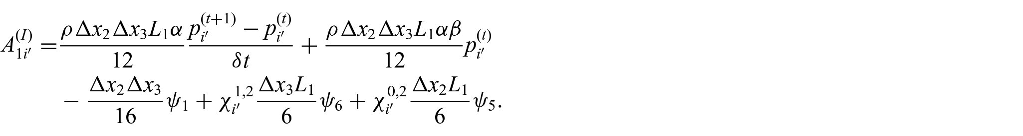
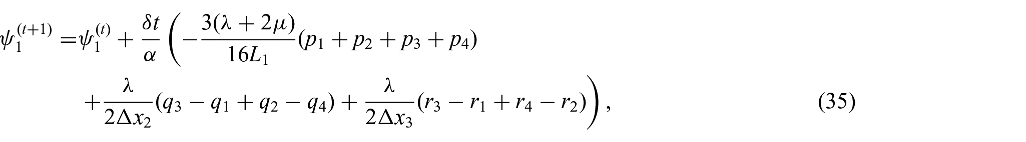
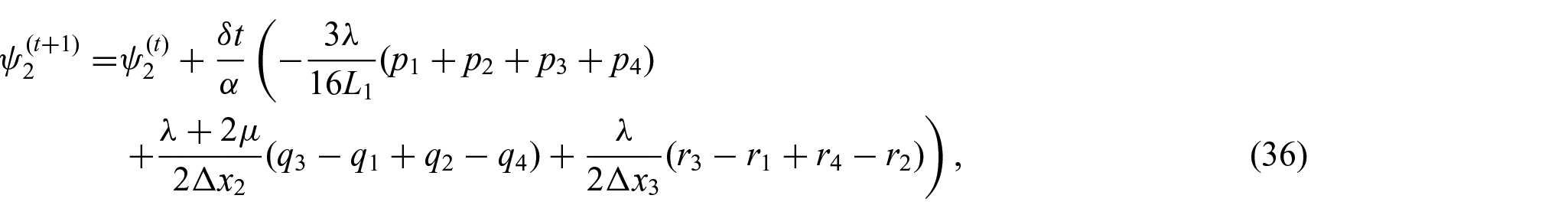
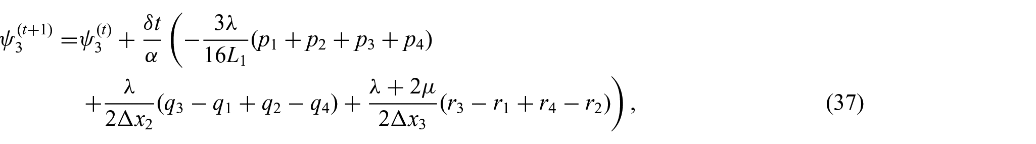
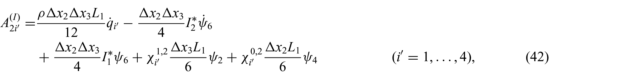
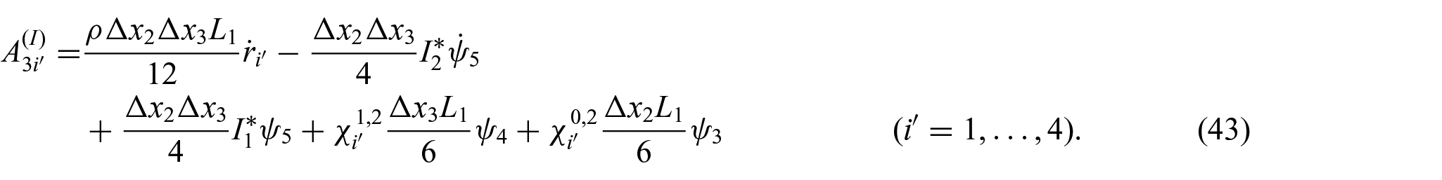
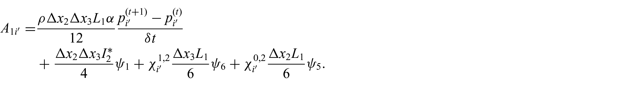
and where $\lceil ·\rceil$ denotes the ceiling function. Similarly, for each IE, the right-hand side of (11)–(13) become

$$\begin{array}{c}{A}_{1i\prime }^{(I)}=\frac{\rho \Delta x_2\Delta x_3{L}_1}{12}\alpha ({\stackrel{·}{p}}_{i\prime }+\beta p_{i\prime })\hfill \\ -\frac{\Delta x_2\Delta x_3}{4}(\frac{L_1}{3c}{\stackrel{·}{\psi }}_1+\frac{1}{4}{\psi }_1)+{\chi }_{i\prime }^{1,2}\frac{\Delta x_3{L}_1}{6}{\psi }_6+{\chi }_{i\prime }^{0,2}\frac{\Delta x_2{L}_1}{6}{\psi }_5(i\prime =1,\dots ,4),\hfill \end{array}$$

(24)

$$\begin{array}{c}{A}_{2i\prime }^{(I)}=\frac{\rho \Delta x_2\Delta x_3{L}_1}{12}\alpha ({\stackrel{·}{q}}_{i\prime }+\beta q_{i\prime })\hfill \\ -\frac{\Delta x_2\Delta x_3}{4}(\frac{L_1}{3c}{\stackrel{·}{\psi }}_6+\frac{1}{4}{\psi }_6)+{\chi }_{i\prime }^{1,2}\frac{\Delta x_3{L}_1}{6}{\psi }_2+{\chi }_{i\prime }^{0,2}\frac{\Delta x_2{L}_1}{6}{\psi }_4(i\prime =1,\dots ,4),\hfill \end{array}$$

(25)

and

$$\begin{array}{c}{A}_{3i\prime }^{(I)}=\frac{\rho \Delta x_2\Delta x_3{L}_1}{12}\alpha ({\stackrel{·}{r}}_{i\prime }+\beta r_{i\prime })\hfill \\ -\frac{\Delta x_2\Delta x_3}{4}(\frac{L_1}{3c}{\stackrel{·}{\psi }}_5+\frac{1}{4}{\psi }_5)+{\chi }_{i\prime }^{1,2}\frac{\Delta x_3{L}_1}{6}{\psi }_4+{\chi }_{i\prime }^{0,2}\frac{\Delta x_2{L}_1}{6}{\psi }_3(i\prime =1,\dots ,4),\hfill \end{array}$$

(26)

where $\alpha ,\beta$ are the stretching function parameters from equation (4) (which have no spatial dependence for this constant stretching case). To obtain an explicit form, Euler’s method is used and, for example, from (20) we can write

$$A_{1i\prime }^{(F)}=\frac{\rho \Delta x_1\Delta x_2\Delta x_3}{8}\frac{p_{i\prime }^{(t+1)}-p_{i\prime }^{(t)}}{\delta t}+{\chi }_{i\prime }^{0,2}\frac{\Delta x_2\Delta x_3}{4}{\psi }_1+{\chi }_{i\prime }^{1,2}\frac{\Delta x_1\Delta x_3}{4}{\psi }_6+{\chi }_{i\prime }^{0,4}\frac{\Delta x_1\Delta x_2}{4}{\psi }_5,$$

and from (24), we obtain

$$\begin{array}{c}{A}_{1i\prime }^{(I)}=\frac{\rho \Delta x_2\Delta x_3{L}_1\alpha }{12}\frac{p_{i\prime }^{(t+1)}-p_{i\prime }^{(t)}}{\delta t}+\frac{\rho \Delta x_2\Delta x_3{L}_1\alpha \beta }{12}{p}_{i\prime }^{(t)}\hfill \\ -\frac{\Delta x_2\Delta x_3}{16}{\psi }_1+{\chi }_{i\prime }^{1,2}\frac{\Delta x_3{L}_1}{6}{\psi }_6+{\chi }_{i\prime }^{0,2}\frac{\Delta x_2{L}_1}{6}{\psi }_5.\hfill \end{array}$$

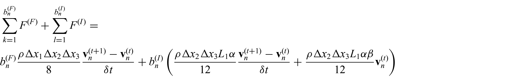
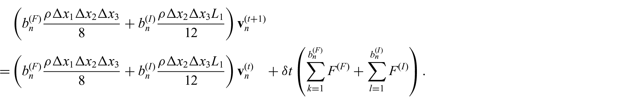
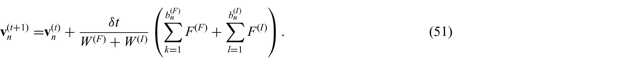
To calculate the velocities at a global level, the FE and IE approximations can be recombined

$$\begin{array}{c}\sum _{k=1}^{b_n^{(F)}}{F}^{(F)}+\sum _{l=1}^{b_n^{(I)}}{F}^{(I)}=\hfill \\ b_n^{(F)}\frac{\rho \Delta x_1\Delta x_2\Delta x_3}{8}\frac{{\mathbf{v}}_n^{(t+1)}-{\mathbf{v}}_n^{(t)}}{\delta t}+b_n^{(I)}(\frac{\rho \Delta x_2\Delta x_3{L}_1\alpha }{12}\frac{{\mathbf{v}}_n^{(t+1)}-{\mathbf{v}}_n^{(t)}}{\delta t}+\frac{\rho \Delta x_2\Delta x_3{L}_1\alpha \beta }{12}{\mathbf{v}}_n^{(t)})\hfill \end{array}$$

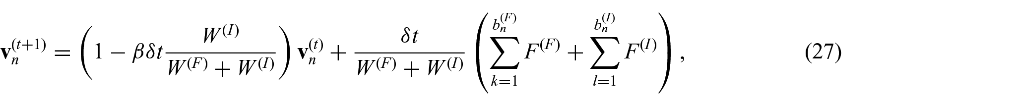
where $b_n^{(F)}$ is the number of FEs that share global node $n$ as a vertex, $b_n^{(I)}$ is the number of IEs that share global node $n$ as a vertex, $F^{(F)}$ is a vector whose entries are the combination of stress terms used in (20)–(22) when global node $n$ is local node $i\prime$ in a FE, and $F^{(I)}$ is a vector whose entries are the combination of stress terms used in (24)–(26) when global node $n$ is local node $i\prime$ in an IE. Thus, the evolution of the velocity can be written in the form

$${\mathbf{v}}_n^{(t+1)}=(1-\beta \delta t\frac{W^{(I)}}{W^{(F)}+W^{(I)}}){\mathbf{v}}_n^{(t)}+\frac{\delta t}{W^{(F)}+W^{(I)}}(\sum _{k=1}^{b_n^{(F)}}{F}^{(F)}+\sum _{l=1}^{b_n^{(I)}}{F}^{(I)}),$$

(27)

where

$$W^{(F)}=b_n^{(F)}\frac{\rho \Delta x_1\Delta x_2\Delta x_3}{8},W^{(I)}=b_n^{(I)}\frac{\rho \Delta x_2\Delta x_3{L}_1\alpha }{12}.$$

(28)

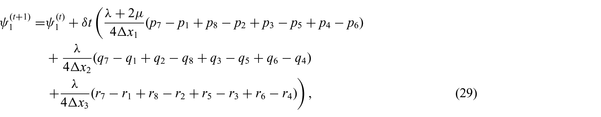
In a similar manner, the FE stress equations which are derived from (6) yield the explicit forms

$$\begin{array}{c}{\psi }_1^{(t+1)}={\psi }_1^{(t)}+\delta t(\frac{\lambda +2\mu }{4\Delta x_1}(p_7-p_1+p_8-p_2+p_3-p_5+p_4-p_6)\hfill \\ +\frac{\lambda }{4\Delta x_2}(q_7-q_1+q_2-q_8+q_3-q_5+q_6-q_4)\hfill \\ +\frac{\lambda }{4\Delta x_3}(r_7-r_1+r_8-r_2+r_5-r_3+r_6-r_4)),\hfill \end{array}$$

(29)

$$\begin{array}{c}{\psi }_2^{(t+1)}={\psi }_2^{(t)}+\delta t(\frac{\lambda }{4\Delta x_1}(p_7-p_1+p_8-p_2+p_3-p_5+p_4-p_6)\hfill \\ +\frac{\lambda +2\mu }{4\Delta x_2}(q_7-q_1+q_2-q_8+q_3-q_5+q_6-q_4)\hfill \\ +\frac{\lambda }{4\Delta x_3}(r_7-r_1+r_8-r_2+r_5-r_3+r_6-r_4)),\hfill \end{array}$$

(30)

$$\begin{array}{c}{\psi }_3^{(t+1)}={\psi }_3^{(t)}+\delta t(\frac{\lambda }{4\Delta x_1}(p_7-p_1+p_8-p_2+p_3-p_5+p_4-p_6)\hfill \\ +\frac{\lambda }{4\Delta x_2}(q_7-q_1+q_2-q_8+q_3-q_5+q_6-q_4)\hfill \\ +\frac{\lambda +2\mu }{4\Delta x_3}(r_7-r_1+r_8-r_2+r_5-r_3+r_6-r_4)),\hfill \end{array}$$

(31)

$$\begin{array}{c}{\psi }_4^{(t+1)}={\psi }_4^{(t)}+\delta t(\frac{\mu }{4\Delta x_2}(r_7-r_1+r_2-r_8+r_3-r_5+r_6-r_4)\hfill \\ +\frac{\mu }{4\Delta x_3}(q_7-q_1+q_8-q_2+q_5-q_3+q_6-q_4)),\hfill \end{array}$$

(32)

$$\begin{array}{c}{\psi }_5^{(t+1)}={\psi }_5^{(t)}+\delta t(\frac{\mu }{4\Delta x_1}(r_7-r_1+r_8-r_2+r_3-r_5+r_4-r_6)\hfill \\ +\frac{\mu }{4\Delta x_3}(p_7-p_1+p_8-p_2+p_5-p_3+p_6-p_4)),\hfill \end{array}$$

(33)

$$\begin{array}{c}{\psi }_6^{(t+1)}={\psi }_6^{(t)}+\delta t(\frac{\mu }{4\Delta x_1}(q_7-q_1+q_8-q_2+q_3-q_5+q_4-q_6)\hfill \\ +\frac{\mu }{4\Delta x_2}(p_7-p_1+p_2-p_8+p_3-p_5+p_6-p_4)).\hfill \end{array}$$

(34)

For each IE we have

$$\begin{array}{c}{\psi }_1^{(t+1)}={\psi }_1^{(t)}+\frac{\delta t}{\alpha }(-\frac{3(\lambda +2\mu )}{16L_1}(p_1+p_2+p_3+p_4)\hfill \\ +\frac{\lambda }{2\Delta x_2}(q_3-q_1+q_2-q_4)+\frac{\lambda }{2\Delta x_3}(r_3-r_1+r_4-r_2)),\hfill \end{array}$$

(35)

$$\begin{array}{c}{\psi }_2^{(t+1)}={\psi }_2^{(t)}+\frac{\delta t}{\alpha }(-\frac{3\lambda }{16L_1}(p_1+p_2+p_3+p_4)\hfill \\ +\frac{\lambda +2\mu }{2\Delta x_2}(q_3-q_1+q_2-q_4)+\frac{\lambda }{2\Delta x_3}(r_3-r_1+r_4-r_2)),\hfill \end{array}$$

(36)

$$\begin{array}{c}{\psi }_3^{(t+1)}={\psi }_3^{(t)}+\frac{\delta t}{\alpha }(-\frac{3\lambda }{16L_1}(p_1+p_2+p_3+p_4)\hfill \\ +\frac{\lambda }{2\Delta x_2}(q_3-q_1+q_2-q_4)+\frac{\lambda +2\mu }{2\Delta x_3}(r_3-r_1+r_4-r_2)),\hfill \end{array}$$

(37)

$${\psi }_4^{(t+1)}={\psi }_4^{(t)}+\frac{\delta t}{\alpha }(\frac{\mu }{2\Delta x_2}(r_3-r_1+r_2-r_4)+\frac{\mu }{2\Delta x_3}(q_3-q_1+q_4-q_2)),$$

(38)

$${\psi }_5^{(t+1)}={\psi }_5^{(t)}+\frac{\delta t}{\alpha }(-\frac{3\mu }{16L_1}(r_1+r_2+r_3+r_4)+\frac{\mu }{2\Delta x_3}(p_3-p_1+p_4-p_2)),$$

(39)

and

$${\psi }_6^{(t+1)}={\psi }_6^{(t)}+\frac{\delta t}{\alpha }(-\frac{3\mu }{16L_1}(q_1+q_2+q_3+q_4)+\frac{\mu }{2\Delta x_2}(p_3-p_1+p_2-p_4)).$$

(40)

4. Spatially dependent stretching

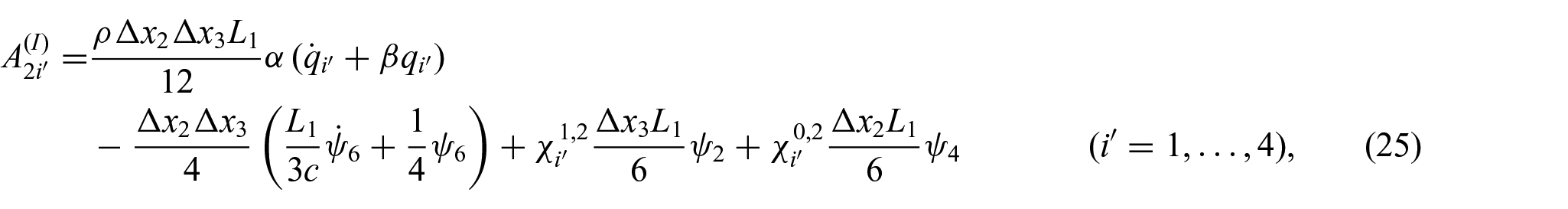
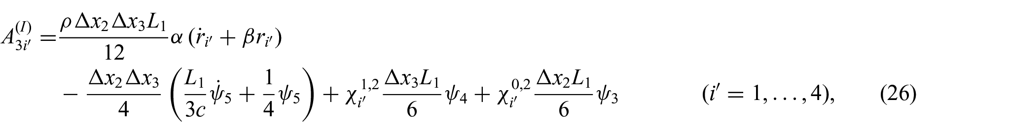
As attention is restricted in this paper to the reflection coefficient from the $x_2$ – $x_3$ plane (see Figure 2), then the PML will only stretch along the $x_1$ -axis and so we can set $s_2=s_3=1$ . The basis functions, test functions and mappings are still defined as in the constant stretching case and the expressions for the FE given by (20)–(22) remain unchanged. A lengthy derivation given in [43] eventually gives rise to the IE time-domain approximations

$$\begin{array}{c}{A}_{1i\prime }^{(I)}=\frac{\rho \Delta x_2\Delta x_3{L}_1}{12}{\stackrel{·}{p}}_{i\prime }-\frac{\Delta x_2\Delta x_3}{4}{I}_2^{*}{\stackrel{·}{\psi }}_1\hfill \\ +\frac{\Delta x_2\Delta x_3}{4}{I}_1^{*}{\psi }_1+{\chi }_{i\prime }^{1,2}\frac{\Delta x_3{L}_1}{6}{\psi }_6+{\chi }_{i\prime }^{0,2}\frac{\Delta x_2{L}_1}{6}{\psi }_5(i\prime =1,\dots ,4),\hfill \end{array}$$

(41)

$$\begin{array}{c}{A}_{2i\prime }^{(I)}=\frac{\rho \Delta x_2\Delta x_3{L}_1}{12}{\stackrel{·}{q}}_{i\prime }-\frac{\Delta x_2\Delta x_3}{4}{I}_2^{*}{\stackrel{·}{\psi }}_6\hfill \\ +\frac{\Delta x_2\Delta x_3}{4}{I}_1^{*}{\psi }_6+{\chi }_{i\prime }^{1,2}\frac{\Delta x_3{L}_1}{6}{\psi }_2+{\chi }_{i\prime }^{0,2}\frac{\Delta x_2{L}_1}{6}{\psi }_4(i\prime =1,\dots ,4),\hfill \end{array}$$

(42)

and

$$\begin{array}{c}{A}_{3i\prime }^{(I)}=\frac{\rho \Delta x_2\Delta x_3{L}_1}{12}{\stackrel{·}{r}}_{i\prime }-\frac{\Delta x_2\Delta x_3}{4}{I}_2^{*}{\stackrel{·}{\psi }}_5\hfill \\ +\frac{\Delta x_2\Delta x_3}{4}{I}_1^{*}{\psi }_5+{\chi }_{i\prime }^{1,2}\frac{\Delta x_3{L}_1}{6}{\psi }_4+{\chi }_{i\prime }^{0,2}\frac{\Delta x_2{L}_1}{6}{\psi }_3(i\prime =1,\dots ,4).\hfill \end{array}$$

(43)

Here

$$I_1^{*}=\underset{X_1\to \infty }{lim}{\int }_{L_1}^{X_1}(\frac{{\beta }_1(x_1)}{c}-\frac{1}{x_1})\frac{1}{{\alpha }_1(x_1)}{\left(\frac{L_1}{x_1}\right)}^4\mathrm{d}{x}_1$$

(44)

$$I_2^{*}=\underset{X_1\to \infty }{lim}{\int }_{L_1}^{X_1}\frac{1}{{\alpha }_1(x_1)c}{\left(\frac{L_1}{x_1}\right)}^4\mathrm{d}{x}_1,$$

(45)

where we choose

$${\alpha }_1(x_1)=1+\overline{\alpha }{(x_1-L_1)}^m$$

(46)

$${\beta }_1(x_1)=\overline{\beta }{(x_1-L_1)}^n$$

(47)

with

$$\overline{\alpha }=\frac{\overline{\overline{\alpha }}}{L_1^m}\frac{X_1}{X_1-L_1},$$

(48)

$$\overline{\beta }=\frac{c}{{(X_1-L_1)}^{n+1}},$$

(49)

and where $\overline{\overline{\alpha }}$ is some constant that can be used to fine tune the PML (see [43] for further details and justification). Note that $m$ and $n$ must be chosen carefully so that $I_1^{*}$ and $I_2^{*}$ converge to non-zero constants as $X_1\to \infty$ . As before, there exists a suitable parameter regime which justifies the diagonalisation of the velocity coefficient matrix (which is necessary to arrive at these explicit forms of $A$ ). It transpires that $I_2^{*}$ is subject to two conditions: $I_2^{*}<<\rho L_{1}c/3\mu$ and $I_2^{*}<<4L_1\mu /3c(\lambda +2\mu )$ . By non-dimensionalising with respect to the spatial variable so that ${\tilde{x}}_1=x_1/L_1$ , equation (45) can be rewritten

$$I_2^{*}=\frac{L_1}{c}\underset{X_1\to \infty }{lim}{\int }_1^{X_1/L_1}\frac{1}{{\alpha }_1(L_1{\tilde{x}}_1)}{\left(\frac{1}{{\tilde{x}}_1}\right)}^4\mathrm{d}{\tilde{x}}_1.$$

Here we see that the factor $L_1/c$ is common to both sides of the second inequality, and so the integral in $I_2^{*}$ is constrained by the material properties of the volume (similar to the constant stretching case) and, hence, must be much smaller than $4c_s^2/3c_p^2$ . On further inspection, it is shown in [43] that the integral term in equation (45) can be approximated by a function of the free parameter $\overline{\overline{\alpha }}$ . By choosing $\overline{\overline{\alpha }}>1$ , we can ensure that both inequalities hold in the materials of interest (for example, steels and other common engineering metals).

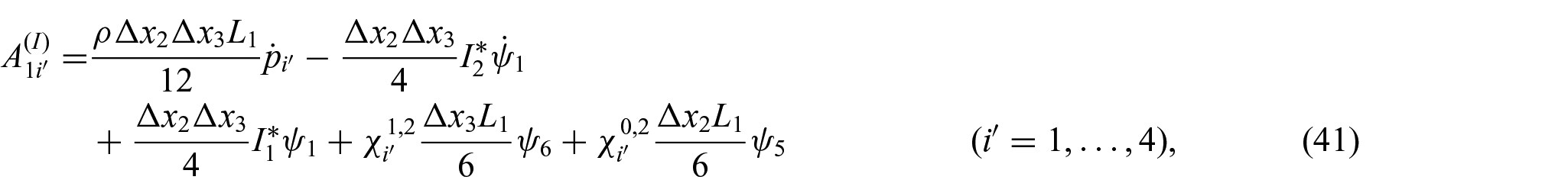
Once again, by implementing Euler’s method, an explicit form for each IE can be obtained, for example, equation (41) becomes

$$\begin{array}{c}{A}_{1i\prime }=\frac{\rho \Delta x_2\Delta x_3{L}_1\alpha }{12}\frac{p_{i\prime }^{(t+1)}-p_{i\prime }^{(t)}}{\delta t}\hfill \\ +\frac{\Delta x_2\Delta x_3{I}_2^{*}}{4}{\psi }_1+{\chi }_{i\prime }^{1,2}\frac{\Delta x_3{L}_1}{6}{\psi }_6+{\chi }_{i\prime }^{0,2}\frac{\Delta x_2{L}_1}{6}{\psi }_5.\hfill \end{array}$$

Now recombining the elements in order to calculate the velocities at a global level gives

$$\sum _{k=1}^{b_n^{(F)}}{F}^{(F)}+\sum _{l=1}^{b_n^{(I)}}{F}^{(I)}=b_n^{(F)}\frac{\rho \Delta x_1\Delta x_2\Delta x_3}{8}\frac{{\mathbf{v}}_n^{(t+1)}-{\mathbf{v}}_n^{(t)}}{\delta t}+b_n^{(I)}\frac{\rho \Delta x_2\Delta x_3{L}_1}{12}\frac{{\mathbf{v}}_n^{(t+1)}-{\mathbf{v}}_n^{(t)}}{\delta t},$$

where $b_n^{(F)}$ is the number of FEs that share global node $n$ as a vertex, $b_n^{(I)}$ is the number of IEs that share global node $n$ as a vertex, $F^{(F)}$ is a vector whose entries are the combination of stress terms used in (20)–(22) when global node $n$ is local node $i\prime$ in a FE, and $F^{(I)}$ is a vector whose entries are the combination of stress terms used in (41)–(43) when global node $n$ is local node $i\prime$ in an IE. Thus, we have

$$\begin{array}{c}(b_n^{(F)}\frac{\rho \Delta x_1\Delta x_2\Delta x_3}{8}+b_n^{(I)}\frac{\rho \Delta x_2\Delta x_3{L}_1}{12}){\mathbf{v}}_n^{(t+1)}\hfill \\ =(b_n^{(F)}\frac{\rho \Delta x_1\Delta x_2\Delta x_3}{8}+b_n^{(I)}\frac{\rho \Delta x_2\Delta x_3{L}_1}{12}){\mathbf{v}}_n^{(t)}+\delta t(\sum _{k=1}^{b_n^{(F)}}{F}^{(F)}+\sum _{l=1}^{b_n^{(I)}}{F}^{(I)}).\hfill \end{array}$$

Letting

$$W^{(F)}=b_n^{(F)}\frac{\rho \Delta x_1\Delta x_2\Delta x_3}{8},W^{(I)}=b_n^{(I)}\frac{\rho \Delta x_2\Delta x_3{L}_1}{12},$$

(50)

then the velocity can be written in the form

$${\mathbf{v}}_n^{(t+1)}={\mathbf{v}}_n^{(t)}+\frac{\delta t}{W^{(F)}+W^{(I)}}(\sum _{k=1}^{b_n^{(F)}}{F}^{(F)}+\sum _{l=1}^{b_n^{(I)}}{F}^{(I)}).$$

(51)

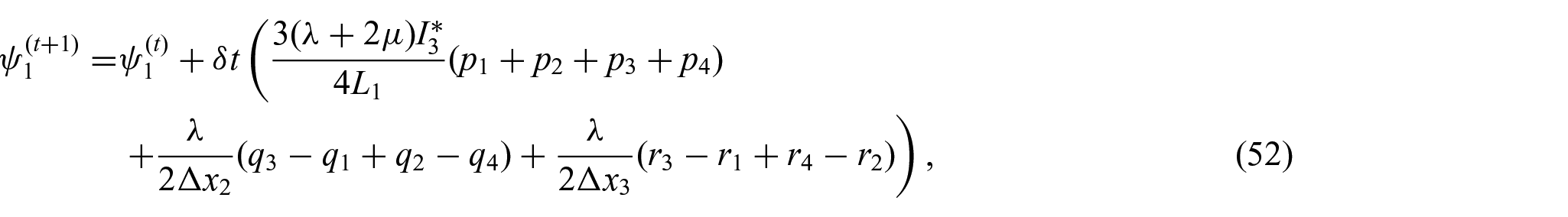
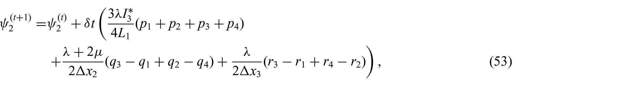
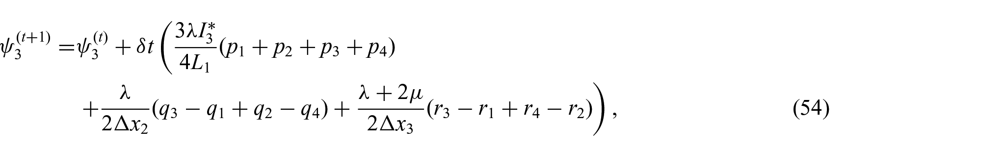
The stress equations can be calculated on an element by element basis, therefore, for each FE, the stress components are given by (29)–(34). For each IE, we can write

$$\begin{array}{c}{\psi }_1^{(t+1)}={\psi }_1^{(t)}+\delta t(\frac{3(\lambda +2\mu )I_3^{*}}{4L_1}(p_1+p_2+p_3+p_4)\hfill \\ +\frac{\lambda }{2\Delta x_2}(q_3-q_1+q_2-q_4)+\frac{\lambda }{2\Delta x_3}(r_3-r_1+r_4-r_2)),\hfill \end{array}$$

(52)

$$\begin{array}{c}{\psi }_2^{(t+1)}={\psi }_2^{(t)}+\delta t(\frac{3\lambda I_3^{*}}{4L_1}(p_1+p_2+p_3+p_4)\hfill \\ +\frac{\lambda +2\mu }{2\Delta x_2}(q_3-q_1+q_2-q_4)+\frac{\lambda }{2\Delta x_3}(r_3-r_1+r_4-r_2)),\hfill \end{array}$$

(53)

$$\begin{array}{c}{\psi }_3^{(t+1)}={\psi }_3^{(t)}+\delta t(\frac{3\lambda I_3^{*}}{4L_1}(p_1+p_2+p_3+p_4)\hfill \\ +\frac{\lambda }{2\Delta x_2}(q_3-q_1+q_2-q_4)+\frac{\lambda +2\mu }{2\Delta x_3}(r_3-r_1+r_4-r_2)),\hfill \end{array}$$

(54)

$${\psi }_4^{(t+1)}={\psi }_4^{(t)}+\delta t(\frac{\mu }{2\Delta x_2}(r_3-r_1+r_2-r_4)+\frac{\mu }{2\Delta x_3}(q_3-q_1+q_4-q_2)),$$

(55)

$${\psi }_5^{(t+1)}={\psi }_5^{(t)}+\delta t(\frac{3\mu I_3^{*}}{4L_1}(r_1+r_2+r_3+r_4)+\frac{\mu }{2\Delta x_3}(p_3-p_1+p_4-p_2)),$$

(56)

and

$${\psi }_6^{(t+1)}={\psi }_6^{(t)}+\delta t(\frac{3\mu I_3^{*}}{4L_1}(q_1+q_2+q_3+q_4)+\frac{\mu }{2\Delta x_2}(p_3-p_1+p_2-p_4)),$$

(57)

where

$$I_3^{*}=\underset{X_1\to \infty }{lim}{\int }_{L_1}^{X_1}(-\frac{1}{x_1}-\frac{{\beta }_1(x_1)}{c})\frac{1}{{\alpha }_1(x_1)}{\left(\frac{L_1}{x_1}\right)}^4\mathrm{d}{x}_1.$$

(58)

5. Results

Having derived PML+IE formulations with constant stretching and spatially dependent stretching, each case was implemented in an explicit FE code using Fortran (see Appendix A for the implementation). A comparison is made between the PML+IE formulation and the FE-only implementation (where the same elastodynamic problem is modelled using hexahedral FEs with stress-free boundary conditions implemented at $x_1=L_1$ ) using a reflection coefficient $p_{\mathrm{refl}}$ , defined as the ratio of the returning reflected wave to the incident wave measured at a node in the centre of the volume. It is given by

$$p_{\mathrm{refl}}=\frac{p_{\max }^{(2)}}{p_{\max }^{(1)}},$$

(59)

where, for a node at position $x^{*}=(a\Delta x_1,b\Delta x_2,b\Delta x_3)$ ,

$$p_{\max }^{(1)}=\underset{t\in [t_i-\delta t_n,t_i+\delta t_n]}{max}|p(t)|,$$

$$p_{\max }^{(2)}=\underset{t\in [t_r-\delta t_n,t_r+\delta t_n]}{max}|p(t)|,$$

where $t_i$ is the number of timesteps taken for the incident wave to first reach this node and $t_r$ is the number of timesteps taken for the reflected wave to return to this node. The $p_{\max }$ values are calculated over a window in time of size $2\delta t_n$ to ensure that the arrival time of the maximum amplitude of the wavefront is accurately captured. We then use this reflection coefficient to find values of the stretching function parameters that minimise the amplitude of the reflected wave. In this work, a steel block ( $c=5690$ m/s, $\rho =7700\mathrm{kg}/{\mathrm{m}}^3$ , $\lambda =97.3$ GPa, $\mu =76$ GPa) that has $n_1=51$ nodes in length and $n_2=n_3=101$ nodes in width and height, is considered, where the nodes are spaced equally ( $\Delta x_1=\Delta x_2=\Delta x_3=1\times {10}^{-5}$ m) and the element side length is chosen to be less than the wavelength/10 (which is shown to be sufficient for satisfactory convergence when choosing first-order linear elements [44]). The height and width of the domain are made much larger than the length of the domain to minimise the effects of the boundaries on the propagating wave. The left boundary elements of the system are excited by the time-limited function $v(t)=(1-\cos 2\pi \mathrm{ft})/2$ for $t<=1/f$ , where $f$ is the excitation frequency (here 54MHz). Each simulation was run for 700 time steps where the time step was given by $\delta t=0.6\Delta x_1/c$ (which obeys the Courant–Friedrichs–Lewy condition), and the reflection coefficient was measured at $x^{*}$ with $a=26$ and $b=51$ , at times $t_i=a\Delta x_1/(c\delta t)$ and $t_r=(2(n_1-1)-a)\Delta x_1/(c\delta t)$ .

5.1. Constant stretching

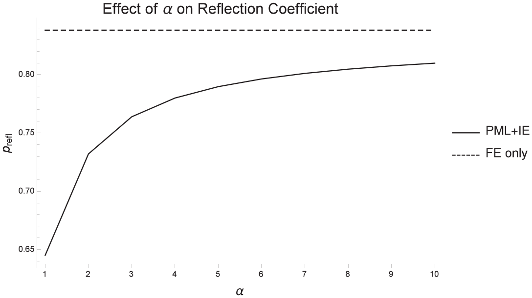
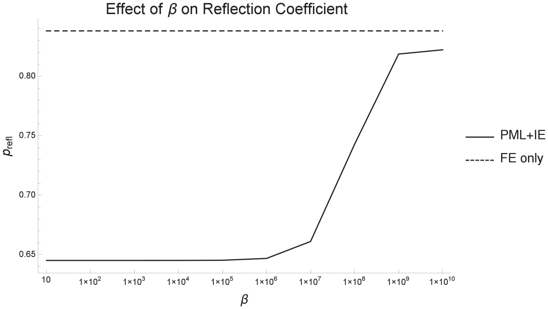
In the case of constant stretching in the PML function, there are two parameters to optimise, namely $\alpha$ and $\beta$ from (4). To minimise the reflection at the domain boundary, we study the effects on the reflected amplitude at a fixed point in the spatial domain as these stretching function parameters are varied. The effect of $\alpha$ is assessed in Figure 5. As $\alpha$ appears in the IE weighting $W^{(I)}$ in (28), it is assumed that it should be of the order $\Delta x_1/L_1$ so that $W^{(I)}$ is similar to $W^{(F)}$ . However, to justify diagonalisation of the velocity coefficient matrix we know that the condition $\alpha >>(\lambda +2\mu )/4\mu$ must hold and so small values close to unity are tested. Figure 5 shows that the reflection coefficient increases as $\alpha$ increases and so the best choice for the stretching function parameter $\alpha$ is given by a value close to 1 (we choose $\alpha =1.001$ ). The effect of $\beta$ is assessed in Figure 6. As $\beta$ appears in the velocity update in (27), it is assumed that the coefficient of $p_n^{(t)}$ should be between $0$ and $1$ . It is clear in Figure 6 that smaller values of $\beta$ produce the lowest reflection coefficients and so we now choose $\beta =10$ .

Figure 5.

The effect of the stretching function parameter $\alpha$ in (4) on the reflection coefficient calculated via (59) for both the FE-only formulation (dashed line) and the PML+IE formulation (full line) with constant stretching for a steel test volume with $n_1=51$ , $n_2=n_3=101$ nodes, with the stretching function parameter $\beta =10$ .

Figure 6.

The effect of the stretching function parameter $\beta$ (from (4)) on the reflection coefficient ( $p_{\mathrm{r}\mathrm{efl}}$ given by (59)) for both the FE-only formulation and the PML+IE formulation with constant stretching for a steel test volume with $n_1=51$ , $n_2=n_3=101$ nodes, with the stretching function parameter $\alpha =0.85$ .

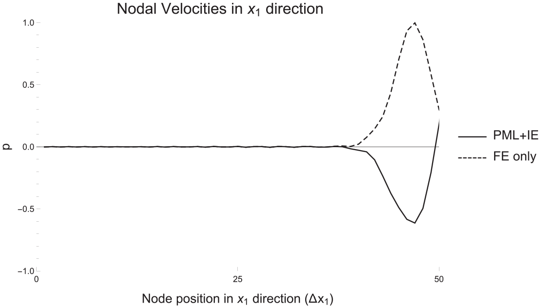
To compare the reflected wave amplitude in the FE-only case and the PML+IE case, the first velocity component $p$ along a horizontal line in the centre of the test volume at a fixed point in time (chosen as the point immediately after reflection from the end of the open end of the volume occurs) is plotted in Figure 7. It can be seen that the reflected wave has a greater amplitude for the case where stress-free boundary conditions are implemented, demonstrating that the PML+IE formulation (with $\alpha =1.001$ and $\beta =10$ ) is successful in reducing the reflection from the boundary. For the same set of parameters, the effect of the domain length in the $x_1$ direction on the reflection coefficient was studied and it was shown that to achieve a similar reduction in reflected amplitude in the case where stress-free boundary conditions are applied at $x_1=L_1$ , the domain had to be more than doubled. Note that the time taken to run the simulations scales approximately linearly with the length of the domain in the $x_1$ direction, as is expected. Importantly, there is little to no difference in runtime between the FE-only formulation and the PML+IE formulation and so the PML+IE formulation can produce a reflection coefficient equal to that of the FE-only formulation by using less than half the number of nodes (memory) and requires only half the runtime.

Figure 7.

Plot of the amplitude of $p$ , the velocity in the $x_1$ direction at a fixed point in time, for a horizontal line of nodes in the middle of a test volume with $n_1=51$ , $n_2=n_3=101$ and with the parameters in equation (4) given by $\alpha =1.0001$ and $\beta =10$ . The plot shows the time immediately after the wave has reached the open end of the test volume and is reflected back into it.

5.2. Spatially dependent stretching

In order to evaluate the integrals present in the formulation of the time-domain IE approximation in the case of non-constant stretching, values $m=1$ and $n=1/4$ are used in (48) and (49) [43]. Therefore, there is only one degree of freedom to explore, namely the stretching function parameter $\overline{\overline{\alpha }}$ . The effect of $\overline{\overline{\alpha }}$ on the reflection coefficient has been assessed by exploring values close to the singularity at $\overline{\overline{\alpha }}=1$ without breaching the conditions $I_2^{*}<<\rho L_{1}c/3\mu$ and $I_2^{*}<<4L_1\mu /3c(\lambda +\mu )$ (see [43]). It transpires that values very close to one in fact produce larger reflection coefficients and so $\overline{\overline{\alpha }}=2$ is chosen for the remaining parametric studies.

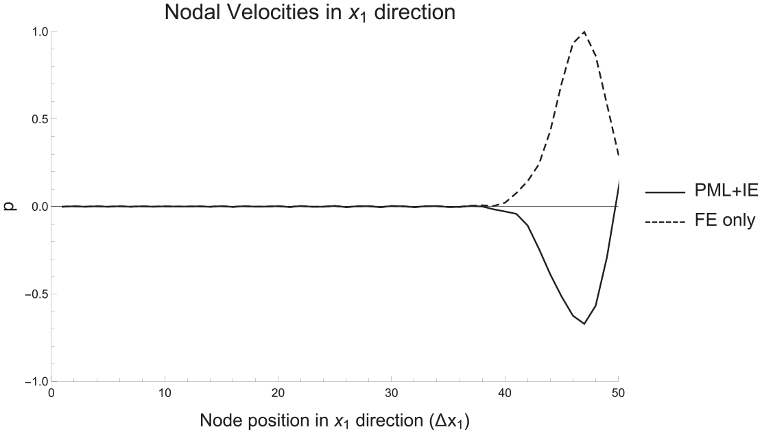
Figure 8 shows the first velocity component $p$ recorded along a horizontal line in the centre of the test volume at a fixed point in time in the case where $\overline{\overline{\alpha }}=2$ . Similar to the results presented in the constant stretching case, it can be seen that the reflected wave has a greater amplitude for the FE-only case (around 1) than for the PML+IE case (close to 0.67), demonstrating that the PML+IE formulation is successful in reducing the reflection from the boundary by around 33%. Similar to the constant stretching case, with $\overline{\overline{\alpha }}=2$ , the PML+IE formulation can produce a reflection coefficient equal to that of the FE-only formulation by using less than half the number of nodes and taking around the half the time to run the simulation [43].

Figure 8.

Plot of the amplitude of $p$ , the velocity in the $x_1$ direction at a fixed point in time, for a horizontal line of nodes in the middle of a $n_1=51$ node long test volume, with $n_2=n_3=101$ , $\overline{\overline{\alpha }}=2$ , $m=1$ and $n=1/4$ . The plot shows the time immediately after the wave has reached the open end of the spatial domain and is reflected back into it.

6. Conclusion

An IE approach has been successfully combined with a PML to produce a new boundary condition for unbounded wave problems in the time domain and a novel formulation for an explicit FE approach using this new PML+IE combination has been presented. Two approaches were considered: the first where the PML stretching function has constant coefficients, and the second where a spatial dependency is retained. Although it would be useful to make comparisons between the PML+IE formulation and IE-only or PML-only formulations, it is not possible to simply switch off one of these components in this formulation. Instead, we compare the reflected wave amplitude with that observed in the case that standard stress-free boundary conditions are applied at the open end of the spatial domain. It was found that in both the constant stretching and spatially dependent stretching cases, the new combined PML+IE is successful in reducing the reflection coefficient by approximately 33%. It was observed that to achieve the same reduction in the reflected wave amplitude using the FE-only approach (with stress-free boundary conditions implemented at the open end) would require double the memory and twice the CPU time. Note here that both formulations produced similar results for the example studied. However, it may be in other scenarios that one approach outperforms the other and this would be an interesting avenue for future work.

Of course, in an ideal world, the new PML+IE formulation presented here would not only reduce the amplitude of the wave reflected from the boundary, but eradicate it completely. In this work, our inability to remove the reflected waveform entirely can in part be attributed to the approximations made in the diagonalisation of the velocity coefficient matrix, which is necessary to compute an efficient explicit FE scheme. However, now that the authors have developed a framework which combines PML and IE boundary conditions, it would be interesting future work to examine the results when an implicit scheme is implemented and quantitatively compare the performance of the method with that of other ABCs.