
Abstract
The main challenging area in the health monitoring of rolling element bearings is the quantification of the spall size using vibration data analysis. This is very crucial for maintenance planning and management decisions. In this article, we present a signal processing scheme for estimating spall sizes in rolling element bearings using autoregressive inverse filtration combined with bearing signal synchronous averaging. The squared envelope of the synchronously averaged signal and its autocorrelation function are used to estimate the spall size. The focus of the preprocessing algorithm using autoregressive inverse filtration resides in enhancing the weak step response events originating from the entry of a rolling element into the spalled region and balancing these with prominent impulse responses which occur when a rolling element strikes the trailing edge. Preprocessing is attained through whitening the shaft order tracked (angular resampled) signal using an autoregressive model based on the shaft synchronously averaged part (autoregressive inverse filtration). Autoregressive inverse filtration is compared to autoregressive filtration based on the raw vibration signal. The selection of the autoregressive model order is realized using Akaike criterion. The efficacy of the two autoregressive filtration algorithms is established by comparing time-domain signals, bearing signal synchronous averages, and their squared envelopes and autocorrelation function. This is done on simulated signals with well-known characteristics and on two sizes of naturally originated and propagated inner race spalls from a high-speed test rig. The sizes of these faults were large in a sense that the rolling element did not bridge over the spall, and this required an adjustment to the size quantification equation to fit this case, which has not been presented before. The combination of autoregressive inverse filtration and the squared envelope of the bearing synchronous averaging gives a superior enhancement to the step response and balances it with the impulse response. This provides the best accuracy in estimating the size of the spall, and unlike other existing algorithms, there exist no need for further processing using wavelets for instance.
Keywords
Introduction
Rolling element bearing fault diagnosis, using vibration data collected via accelerometers, has been the focus of research and industry for decades, where a great number of signal processing algorithms have been developed and implemented successfully. A widely used technique is the envelope analysis or the high-frequency resonance technique (HFRT). 1 Although diagnosing a bearing fault can be done with ease and confidence due to the number of robust algorithms developed,2–5 it may still be a challenging task in some cases, as it is a function of a number of variables, which may mask the bearing defect signal. These include the location of the accelerometer (transfer path between the source of the fault and the sensor); the speed fluctuations; and, in particular, variable speed machines and the loading of the bearings.
A more challenging area is the quantification of the fault size using the vibration data. This is very crucial for maintenance planning and management decisions. Through the novel work of Epps 6 in 1991, it has been established that the vibration response of a defective rolling element bearing (localized faults such as spalls) comprises two main parts (although argued at some instances that a third part exists, but this was not clearly established). The first part of the response comes as the rolling element rolls into the spall. The change of curvature causes a step response in acceleration which results in a low-frequency transient event with a negative slope. The second part of the response results from the impact of the rolling element with the trailing edge of the spall. This causes a sudden change in the rolling direction, which gives a step response in velocity and results in an impulse response in acceleration. The third event, which results from the fully departure of the rolling element and regaining contact with raceway (described as a low-frequency transient with a positive slope—opposite to the entry), was not clearly distinguished due to the dominance of the impact event. Epps showed that the time between the rolling in and the impact (denoted as the time to impact (TTI)) is proportional to the size of the spall and can be used to measure the spall width. A typical example from Epp’s thesis showing the two parts of the vibration signal is shown in Figure 1.

(a) Model of rolling element traveling into a fault and (b) a typical measured response. 6
In 2011, Sawalhi and Randall 7 conducted a number of tests with seeded inner race and outer race faults (two sizes of 0.6 and 1.2 mm). The test rig (bladed fan test rig) was operated at speeds between 800 and 2400 r/min. A typical result from their work for an outer race spall is shown in Figure 2. The step response, associated with the ball entry into the spall, was observed, and the separation between the entry and impact could be directly linked to the size of the fault. It has been indicated that “the entry into the fault could be classified as a step response, with mainly low-frequency content, while the impact on exit excites a much broader band impulse response, with higher frequency content.” Analytical simulation and signal preprocessing and enhancements were proposed to enable quantifying the size of the spall. In addition to providing an analytical model for the two parts, Sawalhi and Randall 8 proposed a number of signal processing alternatives to enhance the weak entry event and estimate the size of the spall. In particular, they proposed the use of signal pre-whitening using autoregressive (AR) modeling for enhancing the entry event, Morlet wavelet analysis 9 to balance the energy of the entry and exit events, and the cepstrum 10 to estimate the spacing between the two events. As the size of the spall was very small compared to the rolling element diameter, it was presumed that the rolling element will bridge over the spall and that the impact occurs when the rolling element is half way through the spall. An equation to estimate the size of the spall based on the number of samples estimated between the entry and impact (TTI) was also derived. 7

Comparison of the raw accelerometer signals for the small (0.6 mm) and large (1.2 mm) outer race faults. 11
A number of researchers have since examined vibration signals for defective bearings at different running speeds and with different spall sizes to enable estimating the fault size. In a 2012 study by Jena and Panigrahi, 12 the authors used analytical wavelet transform (AWT) followed by time marginal integration (TMI) to provide an estimate of a 2.1-mm defect in the inner race at a speed of 1500 r/min. Singh and Kumar 13 used a preprocessing step (multiply the amplitude of the vibration signal by the absolute value) to enhance the step response followed by wavelet analysis to detect defect width over the range of 0.4399–1.4854 mm. Accuracy of estimates were observed to increase with the loading of the bearing. More recently, Moustafa et al., 14 in 2014, introduced instantaneous angular speed (IAS) to aid bearing prognosis. The introduced IAS was tested at very low speed (10–60 r/min) to estimate the fault size of 0.7–6 mm. IAS was found to provide accurate size estimation for normal to high radial loading. Moazenahmadi et al., 15 in their 2014 article, provided insights and more understanding to the path of rolling elements in the defect zone for developing an algorithm to estimate the size of a bearing defect. Their method produced more accurate results that were less biased with operational speed. Ismail and Sawalhi, 11 in 2016, introduced a new technique for extracting the spall size and determining the geometric factor between the extracted size and the actual size without comparing with any reference data. The technique consists of two energy (or root mean square (RMS)) envelopes for the vibration signal and after numerically differentiating this signal using adjustable Savitzky–Golay. Finally Wang et al., 16 in their 2016 work, proposed a system of estimating bearing spall size using a tacho-less synchronous signal averaging (SSA) with respect to the bearing fault characteristic frequency combined with envelope and wavelet analyses of the averaged signals. The proposed algorithm, which was applied directly to the raw vibration signal without preprocessing, was validated using the vibration data from naturally spalled bearings (4.2 and 6.2 mm) in a high-speed bearing test rig (7700 r/min). The presented results showed that the technique is effective in revealing the entry and exit features needed for the size estimation of naturally occurring bearing faults. No preprocessing was attempted before applying the SSA scheme.
In this article, we present a signal processing algorithm to estimate the size of spalls in rolling element bearing using vibration signals. The proposed algorithm includes a whitening process of the shaft order tracked signal using autoregressive inverse filtration (ARIF; i.e. filter coefficients are derived from the shaft synchronous averaged signal). The residual of the ARIF process is then utilized to extract a bearing signal synchronous average (BSSA), whose squared envelope is used to estimate the size of the spall. The selection of AR model order and the validation of the algorithm are demonstrated on simulated signals and on the two naturally originated inner race spalls used in Wang et al. 16 A number of comparisons are made to demonstrate the advantages of the ARIF processes compared to AR filtration on the raw signal and the importance of signal preprocessing prior to using BSSA.
This article is organized as follows: In section “Processing scheme to estimate spall size,” the proposed processing scheme to estimate spall size in rolling element bearing is discussed. This involves presenting the ARIF of the order tracked residual signal and the BSSA procedure. The bearing test rig used to collect experimental data, the type of faults introduced in bearings, and the characteristics of the collected vibration data are discussed in section “Bearing test rig and vibration data.” This section also provides calculation of the spall size in samples. Section “Simulations” presents analytical simulations which are based on characteristics similar to that seen in experimental data. This section also presents the results obtained from applying the processing scheme presented in section “Processing scheme to estimate spall size” on the simulated signals. Section “Experimental results” examines the experimental data when subjected to the processing scheme. Finally, conclusions are given in section “Conclusion.”
Processing scheme to estimate spall size
The proposed processing scheme consists of three main stages of processing. The first stage involves preprocessing an angular sampled (order tracked) version of the raw vibration signal using ARIF. The aim of this preprocessing is to remove the effect of the transfer path and to whiten the vibration signal which then enhances the weak step response and minimizes the dominance of the impulse response. ARIF processing algorithm is discussed and illustrated in section “ARIF and whitening of the shaft order tracked signal.” Results obtained using this proposed algorithm are compared to AR processing applied directly on the raw vibration signal. In the second stage, the residual of the ARIF algorithm is processed to extract a BSSA with respect to a bearing fault characteristic frequency. The essence of this processing is discussed in section “Tacho-less BSSA.” The final stage of processing includes calculating the squared envelope of the BSSA obtained from step 2 for three or more periods and examining it and its autocorrelation function to estimate the size of the spall.
ARIF and whitening of the shaft order tracked signal
Figure 3 describes schematically the ARIF process to enhance the step response and improve the presence and localization of the impulse response.
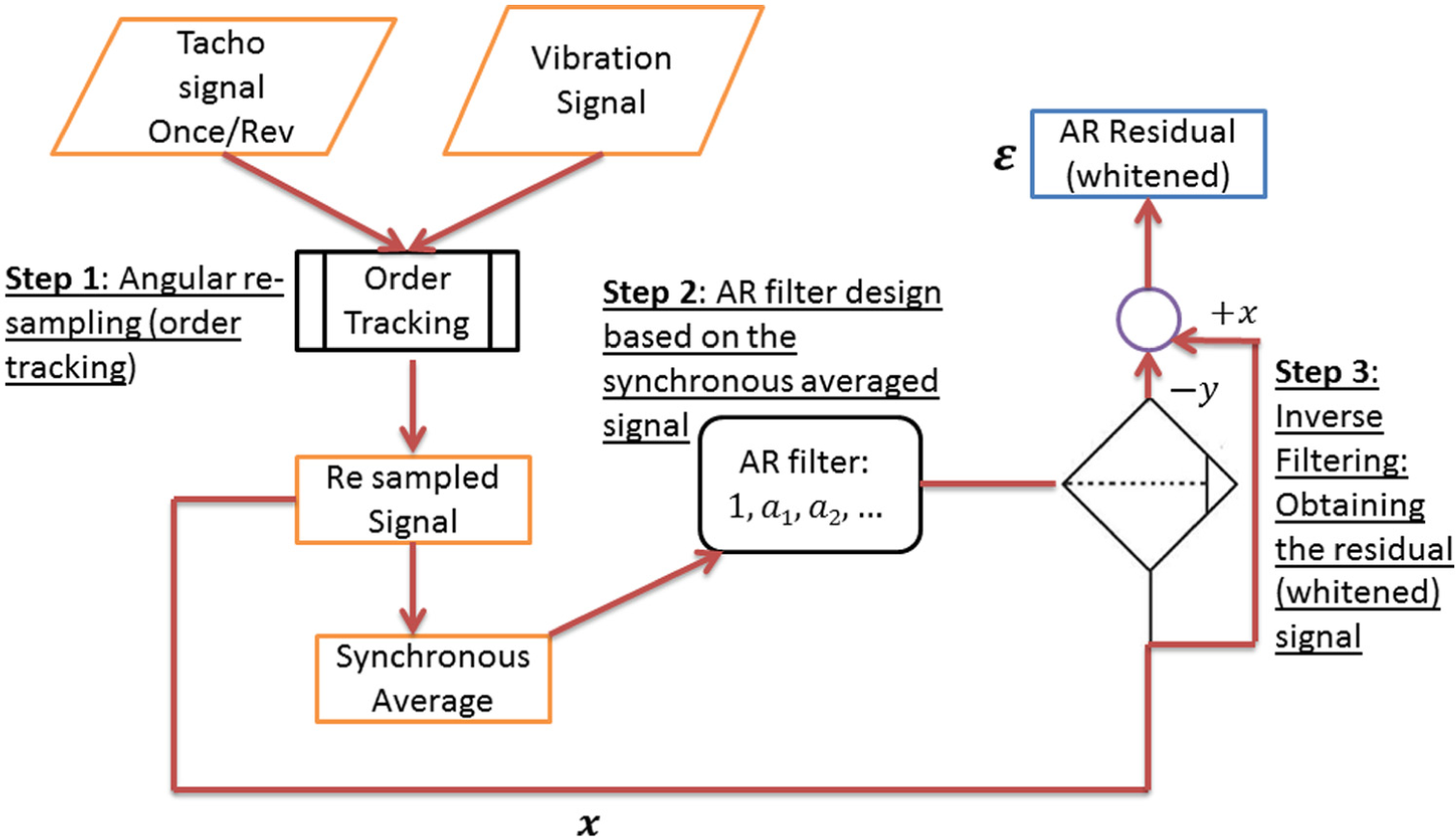
Order tracking and AR inverse filtration to enhance the step response.
In this approach, an AR model is derived using the shaft time synchronous averaged (TSA) signal. The first step in the process includes using the tachometer signal to order track the vibration signal, thus removing any speed fluctuations. The TSA is then obtained through finding the ensemble average of a number of shaft rotations.
The TSA contains all the harmonics of the shaft frequency (shaft orders) and the ringing effects (sinusoidal components) of the structural resonances in the system. This TSA is used to build an AR model using equation (1) presented below. In an AR model, a value at time t is based on a linear combination of prior values (forward prediction), a combination of subsequent values (backward prediction), or both (forward–backward prediction). If x is a data series (zero mean stationary process) of length N and a is the AR parameter array of order p, an AR model Y can then be defined in equation (1) as follows 17
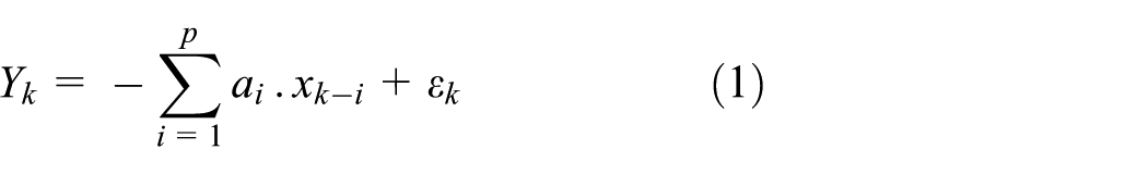
where p is the order of the model and
Several criteria have been proposed to select the optimum (minimum) model order (p) The Akaike Information Criterion (AIC)—one of the most popular measures in the literature—determines the model order p by minimizing an information theoretic function of p;
18

where N is the number of samples and
The “AIC” is only one of many criteria proposed for the selection of the AR order. Another popular criterion is the final prediction error (FPE), which selects the model order p by minimizing the function

The term
In this work, we have adopted AIC to guide the selection of the model order as it is a widely used one. In addition to the filter length criterion mentioned above, the choice of the filter length (p) could be guided subjectively by the duration (length) of the impulse response in samples to capture the excited resonances within the model. More discussion and insights are provided when presenting simulated signals in section “Experimental results.”
Note that the ARIF whitening process ensures that a true AR model is derived for the signal and also ensures a more efficient removal of the masking deterministic components (shaft harmonics and resonance ringing sinusoidal components). Thus, it is anticipated that the ARIF whitening process should provide a better enhancement to the entry event and a better localization to the exit event. The limitation of the ARIF whitening resides in the need of a tachometer signal for order tracking and synchronous average signal calculation. However, this is not seen as an obstacle as order tracking can be realized using phase demodulation or through pseudo tachometer extraction as has been discussed in a number of publications.20,21
Sawalhi and Randall 7 used signal pre-whitening using AR modeling to enhance the step response. The whitening was achieved based on deriving an AR filter coefficients using the raw vibration signal itself. The residual signal (difference between the raw signal and an AR-estimated version) is white in the sense of containing noise and impulses, which has a relatively flat spectrum. This helps in lifting the power of low energy events and thus results in gaining some enhancement. In both simulated and experimental sections, ARIF and AR whitening of the raw vibration signals are compared.
Tacho-less BSSA
Time synchronous averaging (TSA) method is widely used in gear fault diagnosis. 17 This was also used to aid bearing fault diagnostics by applying it on the envelope signal to enhance the bearing fault characteristic features.22,23 Using TSA with rolling element bearings requires a speed reference signal (tachometer) from both the shaft and the cage of the bearing, which is impractical for most machines. 23 In 2005, Bonnardot et al. 20 introduced a method of extracting TSA without any tachometer reference. This was possible using the vibration signals’ instantaneous phase information at a dominant shaft order. 20
Tacho-less BSSA method was mainly utilized in the detection and diagnosis of bearing faults.24,25 The only reference of applying the tacho-less BSSA method to size estimation of spalls has been published recently, 16 where the authors used phase demodulation to extract a speed reference from the inner race ball pass frequency and used this to find the squared envelope of the BSSA to estimate the size of two naturally grown inner race spalls from a test rig running at a high speed. The authors then used band pass filtration and wavelet analysis to estimate the spall size.
In this work, a period timing method (pseudo encoder) 21 is used to extract a tacho reference. In this process, a buffer (filled with zeros) of a size equal to the FFT size of the signals is created. The complex spectrum of interest (band around the characteristic bearing frequency) is then transferred to this buffer (filling in the same lines as in the original spectrum). Finally, the buffer is inversely transformed to the time domain to obtain the reference signal. This signal is a sinusoidal signal whose periods represent the period of passage of the rolling elements across either the inner race or the outer race. The fluctuations between each rolling element passage can be traced using the zero crossing of the consecutive periods, which can be achieved by setting a trigger and identifying the zero-crossings. This signal is then used to order track the signal and obtain a synchronous average.
Bearing test rig and vibration data
Test rig and two naturally grown large spall sizes
The test rig used to generate the data for this work is pictured in Figure 4. It consists of two bearing housings. One of these housings contains the test bearing (angular contact bearing), which is loaded axially through screwing a large nut to the housing. The other bearing housing (reaction bearing housing) contains two angular contact bearings, arranged in tandem, which react to the test load. The test rig is driven by a constant speed motor through a belt-pulley system to give a nominal running speed of around 7700 r/min. The test rig was fitted with a vertical–radial accelerometer (as shown in Figure 4), an axial accelerometer, and a tachometer to get a speed reference. Data were acquired at a sampling rate of 200,000 samples/s (Hz).

Vibration bearing test rig.
The information about the test bearing is listed in Table 1. In total, two main fault sizes were used in the testing as shown in Figure 8(b) and (c). The spalls were initiated from a 0.25-mm notch (Figure 8(a)) across the middle of the inner race (depth of 0.1 mm and a width of 2 mm). The seeded notch was created using electrical discharge machining (EDM) and allowed to propagate circumferentially along the raceway in accelerated endurance tests. The final sizes of the spall (lengths) were about 6.2 (AC3) and 4.2 mm (AC8). Sizes were estimated by counting the number of grids on the pictures shown in Figure 8.
Test bearing parameters.

The rate at which a ball passes a point on the inner race (BPFI) can be found using equation (4)

where
Using the values of Table 1, the BPFI can be approximated as 8.7 times the shaft rotational speed. For the AC3 bearing test, the bearing shaft and the inner race were running at a speed of 6270 r/min (104.5 Hz). The BPFI was estimated at 909.1 Hz, which corresponds to an impact period of about 220 samples (i.e. 200,000/909.1). The AC8 bearing was running at a nominal speed of 7500 r/min (125 Hz), which is significantly higher than the AC3 bearing’s running speed, thus giving a shorter impact period estimated at 184 samples (i.e. 200,000/(8.7 × 125)). The spall lengths of AC8 (4.2 mm) and AC3 (6.2 mm) correspond to about 56% and 82%, respectively, of the pitch distance between two balls (7.49 mm (i.e.
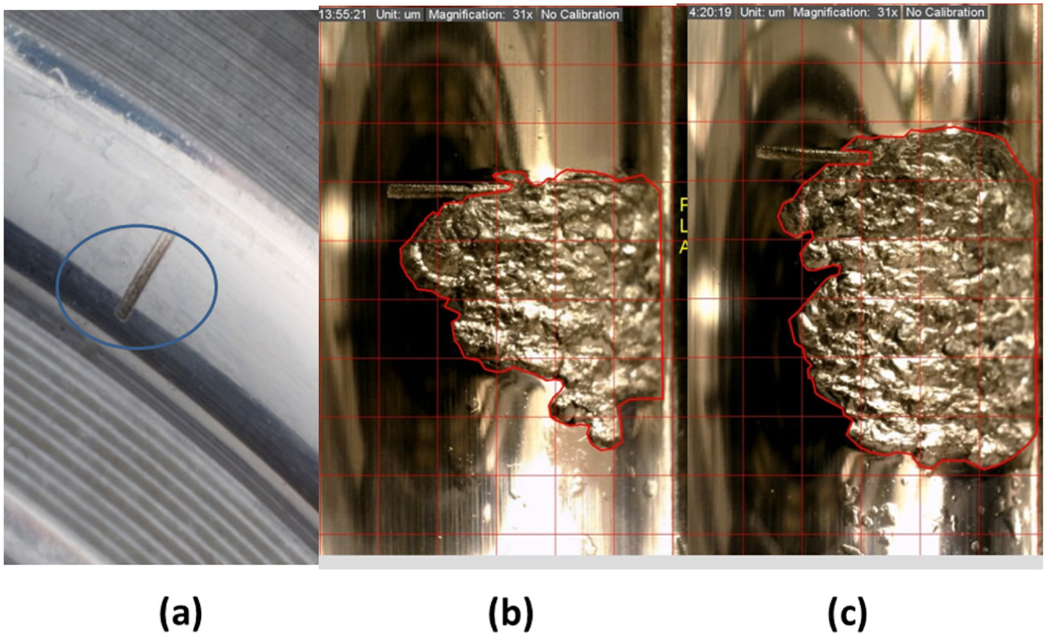
(a) Seed notch, (b) AC8 spall (4.2 mm), and (c) AC3 spall (6.2 mm).
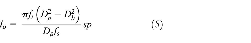
Spall size estimation based on the TTI (number of samples between the roll in and impact)
When the size of the spall is large, the rolling element does not bridge over the spall, and equation (5) presented in Sawalhi and Randall 7 does not give accurate estimation and has to be adjusted. Instead, equations (6) and (7) are to be used for accurate estimates. A schematic comparison between the case presented in Sawalhi and Randall 7 under which equation (5) was derived and a large spall size (as the ones used in this work) is shown in Figure 6.

Spall size estimation based on the number of samples between the roll in (step response) and the impact (impulse response): small spall width (left) and large spall widths (right).
Note that equation (6) has “2” in the denominator and an extra term “x” which is a function of the ball diameter (


where
Based on the measured lengths of spalls and through adjusting with 1.2 mm for the 4.2-mm spall (AC8) and 1.5 mm for the larger 6.2-mm AC3 spall, the spacing between the step and impulse response is estimated at 88 samples and 130 samples, respectively.
Characteristics of the measured signals
Raw vibration signals from the AC8 and AC3 bearings are shown in Figure 7, where the impacts generated by the ball passage over the spall can be clearly seen.
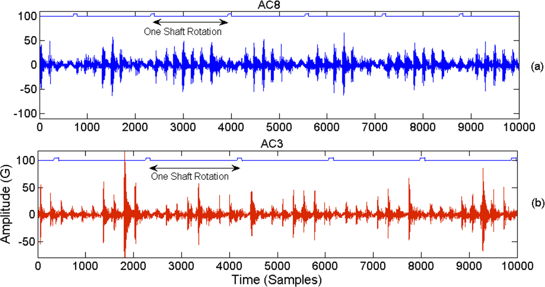
Raw vibration signal with (a) AC8 and (b) AC3.
The amplitude spectra for both AC8 and AC3 signals are shown in Figure 8 with the inner race fault frequency of 1079 Hz (AC8) and 912 Hz (AC3; as marked by the data tip) absolutely dominating. The resonance frequency of the accelerometer is also obvious at around 50 kHz. It is also noted that some resonances are excited below 10 kHz. The AC8 bearing was running at a nominal speed of 7500 r/min, which was significantly higher than the AC3 bearing’s running speed.

Amplitude spectrum for signal with (a) AC8 and (b) AC3.
Simulations
Signal generation
Figure 9 displays a zoomed in version of Figure 7(b), containing three impact periods. As can be seen, there is a lot of noise and interferences in the raw signal between two impacts, so that it is impossible to extract features from the raw signature with the balls entry into and exit from the spalled area on the inner raceway. Because of the high speed used in the test rig (125 Hz), and although the sampling frequency was high (200 kHz), the number of samples between two consecutive impacts are still quite small (around 180 samples). It is most likely that the entry and exit features overlap because the entry-related response does not completely disappear before the exit event starts. This would be similar to the case for the impulse response at exit as it may not die out completely before the step response from the next ball.

Zoomed-in version of the raw vibration signal shown in Figure 7(b).
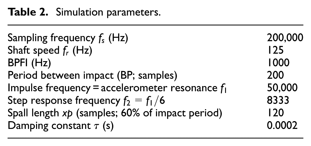
In order to better understand the analysis process, a signal simulation was carried out. The experimental characteristics observed in section “Bearing test rig and vibration data” are mimicked using analytical simulations. Table 2 lists the simulation parameters used when creating simulated signals as described in Table 3. Steps 1–4 of Table 3 are detailed in Sawalhi and Randall. 7 Step 5 was introduced to include a modulation effect. This was realized using a hanning window.
Simulation parameters.
Simulation steps and summary.
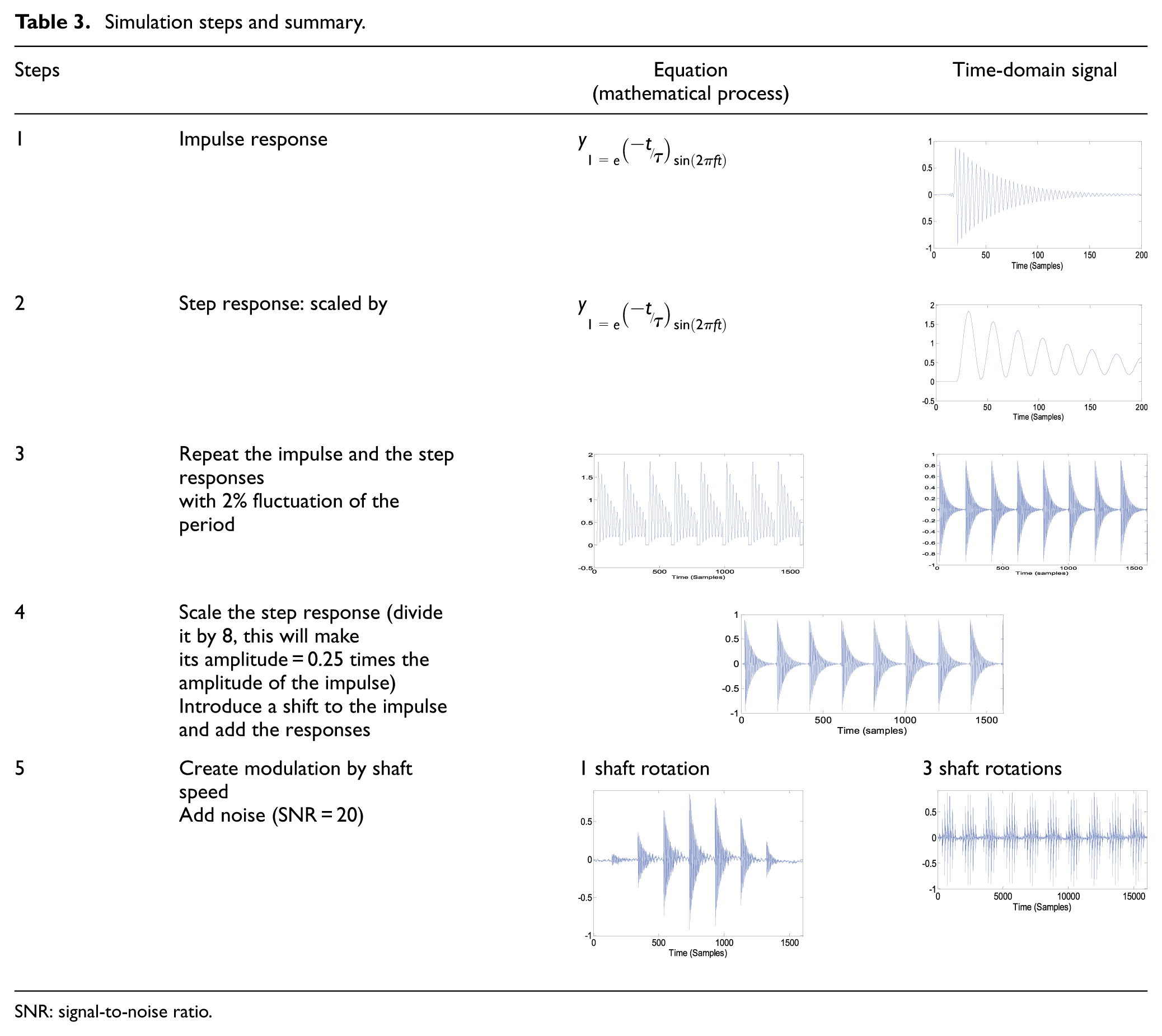
SNR: signal-to-noise ratio.
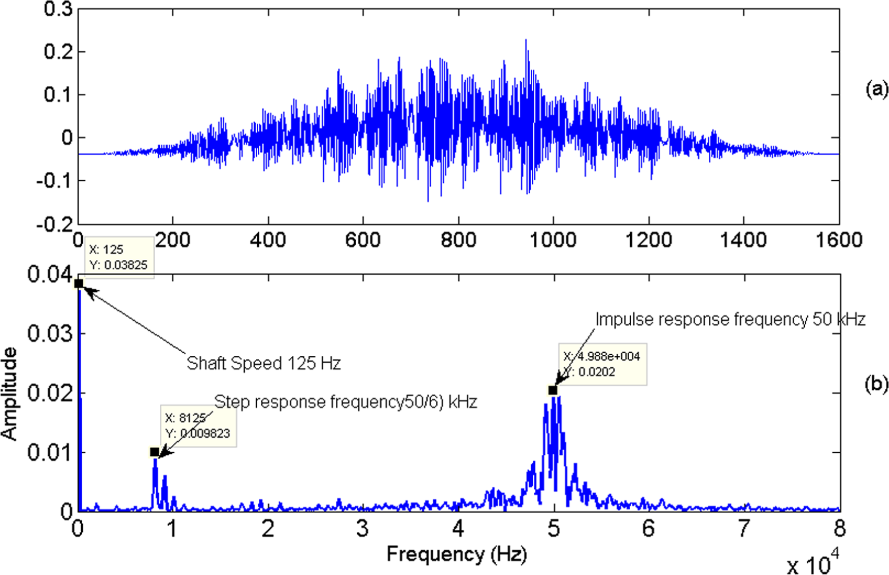
Figures 10 and 11 show the time domain of the simulated signal and its frequency content, respectively.

One shaft rotation of (a) step response, (b) impulse response, and (c) step and impulse responses added with 120 samples delay, SNR = 20 dB. (d) Signal c modulated by the shaft speed.

Frequency content of simulated signal shown in Figure 10(d): (a) full bandwidth (0–100 kHz) showing excited resonances and (b) frequencies 0–1000 Hz showing shaft frequency and the first four harmonics of the BPFI.
Simulated signal processing
Figure 12 shows the shaft TSA and its frequency content, which contains the shaft frequency and the two excited resonances. The implication of this is that the AR model derived from this signal will capture both the shaft frequency and the resonances in the system.
(a) Shaft TSA and (b) frequency content of TSA.
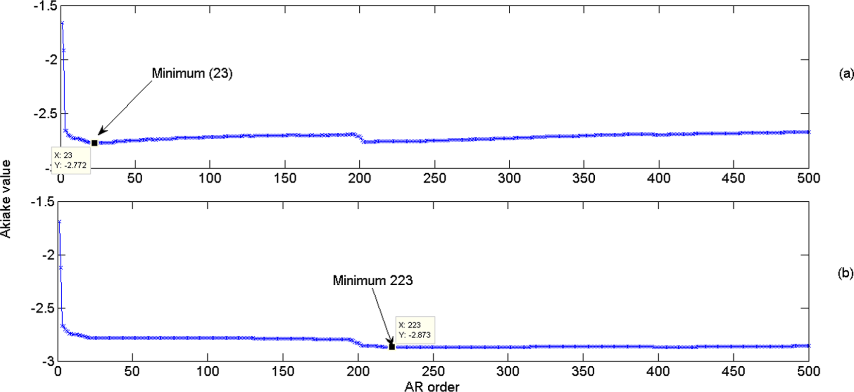
The optimum AR model orders based on Akaike criterion for the ARIF and the one based on the raw signal are plotted in Figure 13. Deriving AR coefficients based on ARIF requires a model order of 23 samples, which translates to about 12% of the impact period. Doing this based on the raw signal requires a filter length of 223 samples, which appears to be of the same order as the impact period.
The residuals of ARIF and AR based on the raw signal over one shaft rotation are plotted in Figure 14. It is seen that both perform well in removing the ringing effect and localizing both the step and impulse responses. However, the ARIF gives a slightly better enhancement for the step response in amplitude and appearance when compared to AR based on the raw signal.

One shaft rotation of (a) simulated signal, (b) residual of AR derived from the raw signal, and (c) residual of AR inverse filtration.
The performance of preprocessing using AR is tested next on the BSSA of the signals. The comparisons between BSSA with no preprocessing to these obtained from the two AR approaches are shown in Figure 15. It is noted that all of the three periods of BSSA extract the step and impulse responses. BSSA over the raw vibration signal (no preprocessing) extracts both the step and impulse responses but with keeping the ringing effect; thus, the localization in terms of the starting positions is missing. AR on the raw signal enhances the step response, localizes the impulse, and balances both events but gives less clear results compared to ARIF. ARIF enhances the step response, localizes the impulse response, and gives a balance between the two responses. Thus, among the three periods of BSSA, the one based on ARIF gives the best result. This can be seen clearly through inspecting the squared envelope signals of the BSSA as shown in Figure 16, where it can be seen clearly that ARIF gives the best result in enhancing the step response and localizing both events, so that spacing can be easily measured to estimate the size of the spall. In the case of no preprocessing and ARIF, further balancing of the events and low-pass filtration for the high-frequency components attached with the impulse events are usually sought as has been the case in Sawalhi and Randall 7 and Wang et al. 16 in which wavelets were employed to aid fault estimation. The one-sided zero-centered autocorrelation of the squared envelope of the BSSA is examined in Figure 17. The 200 and its multiples indicate one impact period, which coincide with the impulse period. The step response location can be seen around sample number 84, giving a spall size of 116 samples, which can be seen as a hump around the location sample 117 in the ARIF and 114 in the AR base. The error in size estimation using ARIF is around 3% for ARIF and 5% for AR based on the raw signal.

Three periods of BSSA (a) calculated on the raw signal, that is, with no preprocessing; (b) using AR filtered on the raw signal; and (c) using AR inverse filtered signal.

Three periods of the squared envelope of BSSA (a) calculated on the raw signal, that is, with no preprocessing; (b) using AR filtered on the raw signal; and (c) using AR inverse filtered signal.

One-sided zero-centered autocorrelation of the squared envelope of the BSSA (a) calculated on the raw signal, that is, with no preprocessing; (b) using AR filtered on the raw signal; and (c) using AR inverse filtered signal.
Experimental results
Preprocessing using AR and ARIF
Figure 18 examines the optimum AR filter order for the AC3 and AC8 for ARIF and AR based on the raw signals. ARIF is optimum at 10 and 49 for AC8 and AC3, respectively. This translates to 6% and 22% of the impacts periods for AC8 and AC3, respectively. No minimum was achieved over the 500 orders selected for AR based on the raw signal, as the Akaike values kept decreasing, but it was noted that there is a very minimal change beyond order 200, so it was used for both AC3 and AC8. As observed earlier in the simulated results, ARIF gives a minimum value (optimum) to select the best filter order, while AR based on the raw signal tends to be the best based on the filter length of the same order as the impact period.
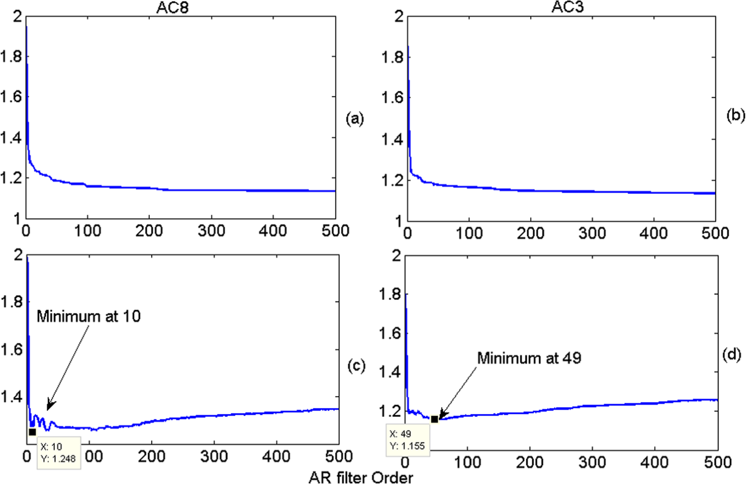
AR filter order selection based on Akaike criterion: (a) AC8 AR on the raw signal, (b) AC3 AR on the raw signal, (c) AC8 AR inverse, and (d) AC3 AR inverse.
Figures 19 and 20 show zoom-in views (about six or seven impacts) from residual signals obtained after preprocessing of AC8 and AC3 signals using AR filtration (both ARIF and AR based on the raw signal). Step responses are noted to be made clear at few instances using both methods of AR and ARIF. However ARIF is observed to give better visual results, and the step responses are obvious at more locations compared to AR based on the raw signals.

A zoom-in showing six impact periods of AC8 signal: (a) order tracked signal, (b) residual of AR derived from the raw signal, and (c) residual of AR inverse filtration.

A zoom-in showing seven impact periods of AC3 signal: (a) order tracked signal, (b) residual of AR derived from the raw signal, and (c) residual of AR inverse filtration.
BSSA and their squared envelopes and autocorrelation functions
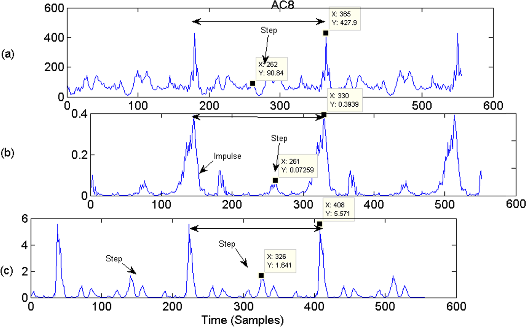
Signals obtained in Figures 19 and 20 were further processed to obtain their BSSA. The results of BSSA are presented in Figures 21 and 22 for AC8 and AC3, respectively. One impact duration, bounded by two impulses, is indicated using a double arrow. The location of the step response is shown in these figures. The signal preprocessed using ARIF provides a much clear identification for the location of the step response compared to the case of no preprocessing and the one where preprocessing was done using AR based on the raw signal. This can be seen and affirmed further by examining the squared enveloped signals of the BSSA in Figures 23 and 24 and their one-sided zero-centered autocorrelation functions in Figures 25 and 26 for AC8 and AC3 signals, respectively. Of particular interest to the aid of spall size are the squared enveloped signals of the BSSA obtained after AR preprocessing as shown in Figure 23 for AC8 and Figure 25 for AC3. ARIF result outperforms the AR processing over the raw signal and the case of no preprocessing. This is clear in particular for the AC3 spall but can also be seen noticeably in the AC8 spall. The use of autocorrelation to estimate the spall size, using ARIF preprocessing, follows a similar trend to what have been discussed in section “Simulations,” where two peaks appear before the impulse location: One represents the step location and the other gives a direct measure for the size of the spall.

AC8: three periods of BSSA (a) calculated on the raw signal, that is, with no preprocessing; (b) using AR filtered on the raw signal; and (c) using AR inverse filtered signal.
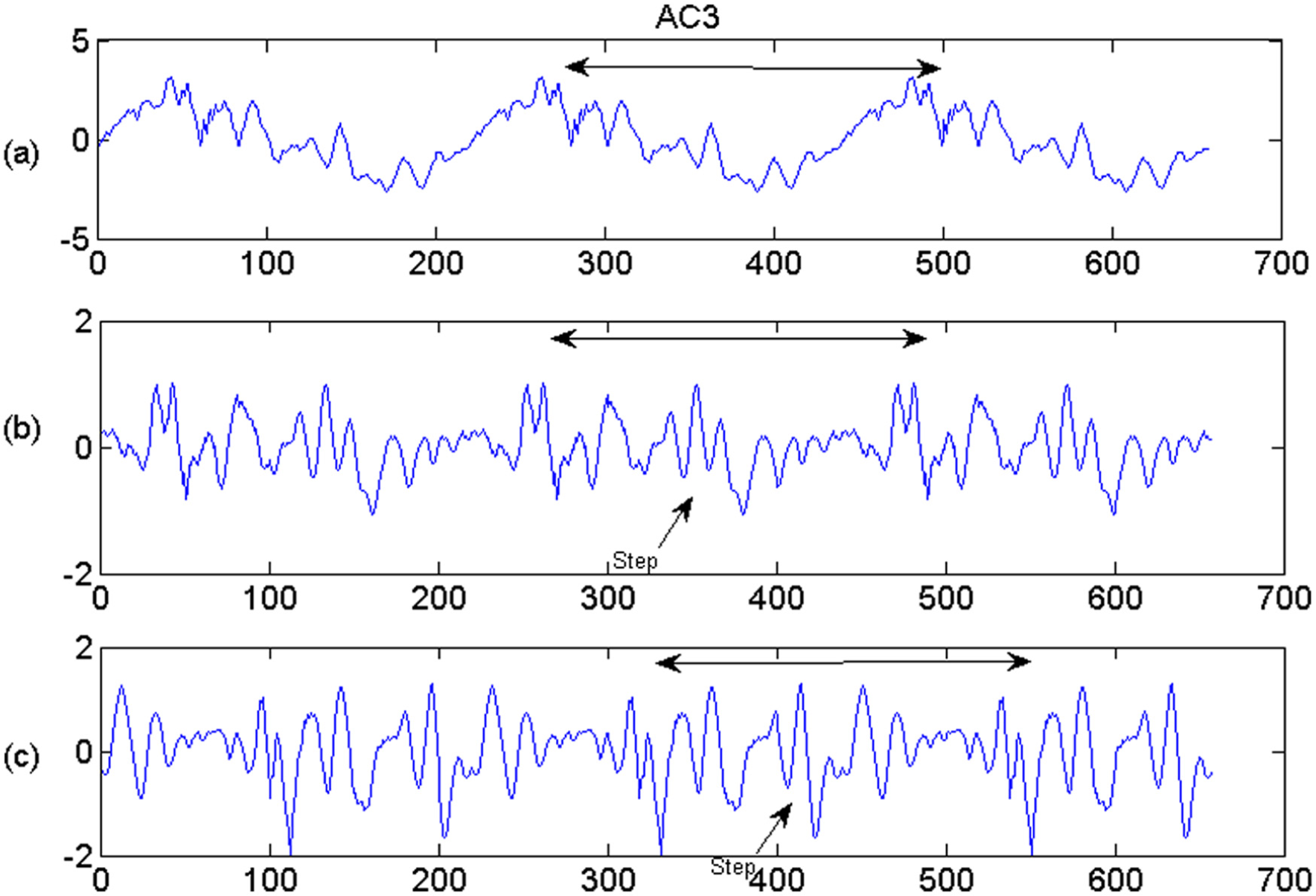
AC3: three periods of BSSA (a) calculated on the raw signal, that is, with no preprocessing; (b) using AR filtered on the raw signal; and (c) using AR inverse filtered signal.
AC8: three periods of (a) bearing synchronous average on the raw signal, (b) bearing synchronous average on the residual of AR raw signal, and (c) bearing synchronous average on the residual of the AR inverse.
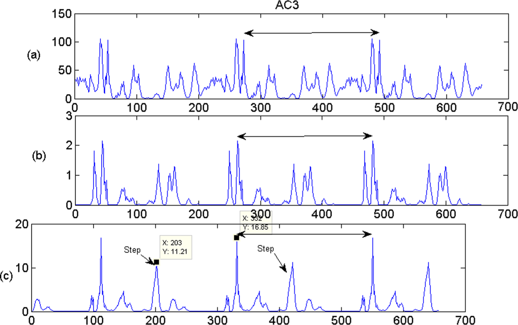
AC3: three periods of (a) bearing synchronous average on the raw signal, (b) bearing synchronous average on the residual of AR raw signal, and (c) bearing synchronous average on the residual of the AR inverse.

AC8: one-sided zero-centered autocorrelation of the squared envelope of the BSSA (a) calculated on the raw signal, that is, with no preprocessing; (b) using AR filtered on the raw signal; and (c) using AR inverse filtered signal.

AC3: one-sided zero-centered autocorrelation of the squared envelope of the BSSA (a) calculated on the raw signal, that is, with no preprocessing; (b) using AR filtered on the raw signal; and (c) using AR inverse filtered signal.
It can be seen through inspecting and comparing these results that ARIF gives the best results in enhancing the step response and balancing and localizing the impulse response. Achieved results are in well agreement with the simulated result presented in the previous section. The spall size of AC8 in samples is estimated at 82 samples (i.e. 408–326 from Figure 23(c) and 186–104 from Figure 25(c)), compared to 88 samples for accurate result (section “Spall size estimation based on the TTI (number of samples between the roll in and impact)”). This gives an error of 4.5%. For the AC3, the spall size in samples is estimated at 129–132 samples (i.e. 332–203 from Figure 24(c) and 220–89 from Figure 26(c)) which matches exactly the expected value of 130 samples as discussed in section “Spall size estimation based on the TTI (number of samples between the roll in and impact).”
Conclusion
A signal processing scheme for estimating the fault size in rolling element bearings has been presented. This is based on using a preprocessing stage using ARIF to remove shaft harmonics and the ringing effects of excited resonances, thus enhancing the step response associated with the spall entries and localizing the impulse response at impact instances. Akaike criterion is utilized to select the AR filter order. The preprocessing stage is followed by a BSSA stage with respect to the ball pass frequency of the fault. The presented processing scheme has been tested on simulated signals and on two inner race spalls for bearings running at high speed. The inner race spalls were naturally grown, and thus, they contained realistic feature of the spalls.
Simulated results were used to test the processing stages and gain an in-depth understanding of the processing. Comparisons were held between preprocessing using ARIF and AR based on the raw signal. The comparison involved comparing the orders of the filters, the time-domain signals, and the bearing signal synchronous averaged signals and their squared enveloped signals and autocorrelation functions to estimate the size of the spall. Simulated results showed a superior performance of fault estimation using ARIF as a preprocessing step, followed by AR based on the raw signal. The case of no preprocessing gave the least accurate estimate as the ringing effect associated with resonances appeared in the BSSA.
For the experimental data, the weak entry event in the cases of the two spall sizes was very hard to observe in the raw data. The use of an ARIF and AR based on the raw signal made it possible to detect some instances of step entries. This was even made better using BSSA on the preprocessed signals and plotting the squared envelopes of the BSSA signals, where localization of both the step and impulse response was achieved. The result quality was much better when preprocessing the signal using ARIF, and in addition to enhancing the step response, the impulse response was better localized. This, in turn, gave a better result and higher accuracy in estimating the size of the spall which were measured directly from the squared envelope signal and using the autocorrelation of the squared enveloped signals.
Footnotes
Acknowledgements
We would like to acknowledge Mr Peter Stanhope of DST Group for his support in the bearing tests. We also thank Dr David Forrester and Dr Peter Frith of DST Group for their support of this work.
Academic Editor: Dong Wang
Declaration of conflicting interests
The author(s) declared no potential conflicts of interest with respect to the research, authorship, and/or publication of this article.
Funding
The author(s) disclosed receipt of the following financial support for the research, authorship, and/or publication of this article: The first author acknowledges the research fund he received from Defence Science and Technology Group to conduct this work.
He also acknowledges the financial support received from Prince Mohammad Bin Fahd University (PMU) for paying the APC.