Sage Journals: Discover world-class research

Abstract

Electromechanical couplings have been reported to play a crucial role in determining important behavior of nonlinear systems. In this study, we analyzed the nonlinear dynamic characteristics of the electromechanical coupling system. First, considering the electromechanical coupling effect of the system, differential equation of the system was obtained by combining the Park equation of a permanent-magnet synchronous motor with the rotor dynamics equation. Then, the coordinate plane projection method was used to analyze the chaotic phenomenon of the electromechanical coupling system. Through calculating the weight value of the 10 projection planes of the electromechanical coupling system, four projection planes with smaller weight values were chosen. Finally, the analysis of the four projection planes of the system indicated that the whole system could reach to the stable state by only controlling the rotational speed in the steady state. In this perspective, the 5-degree-of-freedom system reduced to 2-degree-of-freedom system. Our results would help us create an electromechanical coupling system with a control strategy.

Keywords

Electromechanical coupling chaos coordinate plane projection permanent-magnet synchronous motor nonlinear dynamics

Introduction

Permanent-magnet synchronous motor (PMSM) is of significant interest, particularly for industrial applications such as in the hybrid electric vehicles (HEVs) in the medium-power range owing to its superior features such as compact size, high torque/weight ratio, high torque/inertia ratio, and the absence of rotor losses. The electromechanical coupling phenomenon has been observed in most of the systems. Therefore, recently, coupling has been reported to play a crucial role in determining important evolutions of nonlinear systems.^1–4 The nonlinear dynamic characteristics of the nonlinear electromechanical coupling systems have been extensively investigated and reported in the literature.^5–9 However, in these reports, only the bifurcation and the chaos of the three-dimensional (3D) or four-dimensional (4D) electromechanical coupling systems were analyzed. Few literature reports investigated the nonlinear characteristics of the high-dimensional electromechanical coupling systems. Xue¹⁰ proposed a methodology called SPTR for stability-preserving trajectory reduction. The key is to get the time response curves at first, and divide the curves into complementary pairs respectively, and then map them into a series of spaces with 2 degrees of freedom (DOF) using suitable linear transformation with stability preserving. Based on this methodology, Shao¹¹ proposed the coordinate plane projection (CPP) method to study structure stability of general dynamic system. It divides the system into a pair of complementary subsets, namely, subset X₁ of R² and its complementary subset X₂ of Rⁿ⁻².

Over the past few years, the secure and stable operation of the PMSM, which is an essential requirement of industrial automation manufacturing, has received considerable attention. For instance, Li et al.¹² studied the dynamic characteristics of the PMSM based on the bifurcation and chaos theory. With changing operating parameters, the PMSM exhibits complex behaviors such as limiting cycles and chaos oscillation. Jing et al.¹³ thoroughly investigated the complex dynamics in the PMSM with a nonsmooth air gap, extending the work on the smooth cases. Their theoretical analysis and numerical simulations show some more new results in the PMSM including period-doubling bifurcation, cyclic-fold bifurcation, single- and double-scroll chaotic attractors, ribbon chaotic attractors, as well as intermittent chaos. A linear transformation was used to develop a more explicit form of the PMSM model, and the stability and chaotic behavior of the resulting system were analyzed.¹⁴ Zaher¹⁵ analyzed the stability of the PMSM in the uncontrolled and controlled cases. Hemati and Kwatny¹⁴ presented a compact representation of the machines’ dynamics, considering the nonlinear dynamic characteristics of variable-speed permanent-magnet machines. The systems under investigation were shown to possess multiple equilibria, which profoundly affected their global stability and dynamic characteristics.

The abovementioned literature analyzed the nonlinear characteristics of the PMSMs. In recent years, based on the theoretical analysis of the electromechanical coupling system, a lot of research achievements about bifurcation and chaos of an electromechanical coupling system have been reported. Liu et al.¹⁶ deduced the dynamic equation of a nonlinear electromechanical coupling relative rotation system using the dissipation Lagrange equation. The necessary and sufficient conditions of Hopf bifurcation are given by choosing the electromagnetic stiffness as a bifurcation parameter. Wei et al.¹⁷ investigated the collective dynamics of two coupled PMSMs, indicating that with positive and negative couplings, the coupled PMSMs display rich phenomena such as complete synchronization, amplitude death, antiphase synchronization, and phase-flip transition. R Darula and S Sorokin³ used the multiple scales method to find a steady-state response of the electromechanical system exposed to a harmonic close-resonance mechanical excitation. Taking into account the nonlinearity of the generator shaft and the interaction of mechanics and electrics in the generator set, Niu and Qiu¹⁸ obtained a transient model by combining the Park equations^19,20 of the synchronous generator and mechanical equations. The Hopf bifurcation and the chaos were investigated by the nonlinear mode and Floquet theory.

Above all, there are researchers studying dynamic behaviors of high-dimension system, but that is not the electromechanical coupling system. And there are researchers studying nonlinear dynamic behavior in the electrical motor system, but that is a simplified 3-DOF model. In this study, the nonlinear electromechanical coupling model was established considering the coupling effects of both electrical and mechanical parameters, leading to a five-dimensional (5D) autonomous equation with only two quadratic terms. Because of the large dimensional system, the dynamic characteristics cannot be directly solved and deduced. Based on the CPP method, the dynamic characteristics of the system were analyzed. By calculating the weight of all the 10 projection planes of the electromechanical coupling system, four projection planes with less weight values were chosen and analyzed. By analyzing the four projection planes of the system, the parameters of the system determining desired dynamic characteristics such as stable state were investigated. Finally, computer simulations were performed to verify the presented dynamic behaviors in the electromechanical coupling system.

Model and equations

The transmission system scheme in HEV is shown in Figure 1(a), in which k₁ is the characteristic value of the first planet gear, k₂ is the characteristic value of the second planet gear, i indicates the input shaft, and o the output shaft.

Figure 1.

Transmission and dynamic system: (a) transmission scheme and (b) electromechanical coupling system.

Figure 1(a) shows the variable state combination of brake Z, and clutch C could provide variable transmission mode. When the system is operated in one mode, the motor A or B could be coupled to the mechanical system. Not considering the transmission error and speed ratio, the engine excitation and the road excitation are the load excitation for the simplified electromechanical model.

The simplified electromechanical model of an electromechanical coupling system is shown in Figure 1(b). The electrical part is a PMSM, and the mechanical part has the load excitation indicated by T_l. The two parts are coupled using a shaft, whose stiffness and damp are k and β, respectively.

Let φ₁ be the angle of rotation in PMSM and φ₂ be the angle of rotation in the load system. Then, the torsional angle of the coupling shaft is α = φ₁ − φ₂.

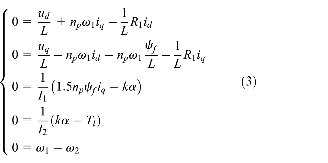
In this study, the transient model of the coupling system was obtained by combining the Park equations^19,20 with mechanical equations

{\begin{matrix} {\overset{\cdot}{i}}_{d} = \frac{u_{d}}{L_{d}} + \frac{L_{q}}{L_{d}} n_{p} ω_{1} i_{q} - \frac{1}{L_{d}} R_{1} i_{d} \\ {\overset{\cdot}{i}}_{q} = \frac{u_{q}}{L_{q}} - \frac{L_{d}}{L_{q}} n_{p} ω_{1} i_{d} - n_{p} ω_{1} \frac{ψ_{f}}{L_{q}} - \frac{1}{L_{q}} R_{1} i_{q} \\ {\overset{\cdot}{ω}}_{1} = \frac{1}{I_{1}} {1.5 n_{p} [ψ_{f} i_{q} + (L_{d} - L_{q}) i_{d} i_{q}] - k α - β (ω_{1} - ω_{2})} \\ {\overset{\cdot}{ω}}_{2} = \frac{1}{I_{2}} (k α + β (ω_{1} - ω_{2}) - T_{l}) \\ \overset{\cdot}{α} = ω_{1} - ω_{2} \end{matrix}

(1)

where i_d, i_q, ω₁, ω₂, and α are the state variables, representing the d-axis stator current, q-axis stator current, motor rotary speed, load rotary speed, and torsional angle, respectively; u_d and u_q are the d-axis and q-axis stator voltage, respectively; I₁ is the rotor inertia of the PMSM; I₂ is the rotor inertia of the load; k is the stiffness of the connecting shaft; β is the damp of the connecting shaft; R₁ is the stator winding resistance; T_l is the external load torque; L_d and L_q are the d-axis and q-axis stator inductors, respectively; ψ_f is the permanent-magnet flux; and n_p is the number of pole-pairs.

Electrical vehicles mainly use surface-mounted PMSMs. Then, L_d = L_q = L. Ignoring the damp of the connecting shaft, namely β = 0, the model equation can be written as

{\begin{matrix} {\overset{\cdot}{i}}_{d} = \frac{u_{d}}{L} + n_{p} ω_{1} i_{q} - \frac{1}{L} R_{1} i_{d} \\ {\overset{\cdot}{i}}_{q} = \frac{u_{q}}{L} - n_{p} ω_{1} i_{d} - n_{p} ω_{1} \frac{ψ_{f}}{L} - \frac{1}{L} R_{1} i_{q} \\ {\overset{\cdot}{ω}}_{1} = \frac{1}{I_{1}} (1.5 n_{p} ψ_{f} i_{q} - k α) \\ {\overset{\cdot}{ω}}_{2} = \frac{1}{I_{2}} (k α - T_{l}) \\ \overset{\cdot}{α} = ω_{1} - ω_{2} \end{matrix}

(2)

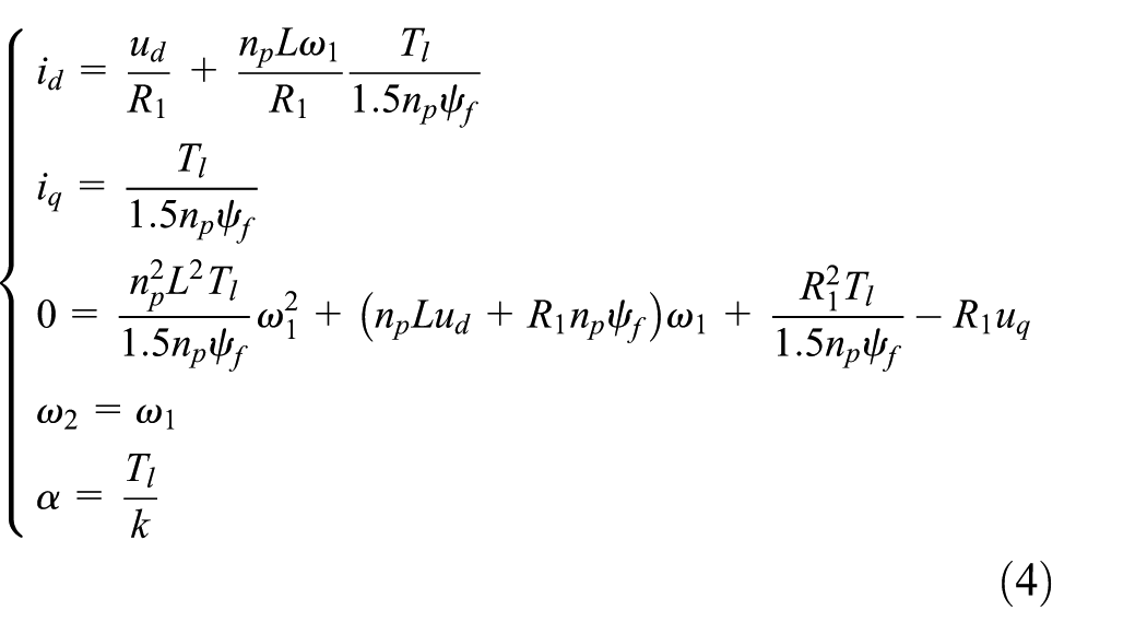
The equilibrium point can be calculated by comparing each equation in system of equation (2) to zero

{\begin{matrix} 0 = \frac{u_{d}}{L} + n_{p} ω_{1} i_{q} - \frac{1}{L} R_{1} i_{d} \\ 0 = \frac{u_{q}}{L} - n_{p} ω_{1} i_{d} - n_{p} ω_{1} \frac{ψ_{f}}{L} - \frac{1}{L} R_{1} i_{q} \\ 0 = \frac{1}{I_{1}} (1.5 n_{p} ψ_{f} i_{q} - k α) \\ 0 = \frac{1}{I_{2}} (k α - T_{l}) \\ 0 = ω_{1} - ω_{2} \end{matrix}

(3)

Then, the following equation can be obtained

{\begin{matrix} i_{d} = \frac{u_{d}}{R_{1}} + \frac{n_{p} L ω_{1}}{R_{1}} \frac{T_{l}}{1.5 n_{p} ψ_{f}} \\ i_{q} = \frac{T_{l}}{1.5 n_{p} ψ_{f}} \\ 0 = \frac{n_{p}^{2} L^{2} T_{l}}{1.5 n_{p} ψ_{f}} ω_{1}^{2} + (n_{p} L u_{d} + R_{1} n_{p} ψ_{f}) ω_{1} + \frac{R_{1}^{2} T_{l}}{1.5 n_{p} ψ_{f}} - R_{1} u_{q} \\ ω_{2} = ω_{1} \\ α = \frac{T_{l}}{k} \end{matrix}

(4)

The Jacobian matrix can be obtained as

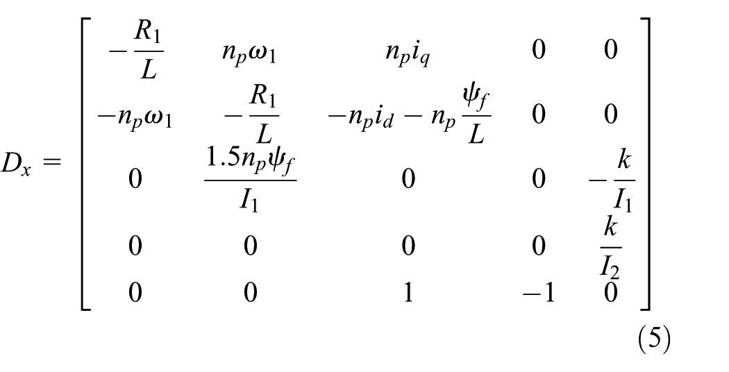
D_{x} = [\begin{matrix} - \frac{R_{1}}{L} & n_{p} ω_{1} & n_{p} i_{q} & 0 & 0 \\ - n_{p} ω_{1} & - \frac{R_{1}}{L} & - n_{p} i_{d} - n_{p} \frac{ψ_{f}}{L} & 0 & 0 \\ 0 & \frac{1.5 n_{p} ψ_{f}}{I_{1}} & 0 & 0 & - \frac{k}{I_{1}} \\ 0 & 0 & 0 & 0 & \frac{k}{I_{2}} \\ 0 & 0 & 1 & - 1 & 0 \end{matrix}]

(5)

The equilibrium point can be obtained from equation (4). Substituting equation (4) into equation (5) and solving the eigenvalue of the Jacobian matrix, the dynamic stability of the system can be analyzed.

Dynamic behaviors of the electromechanical coupling system

First solving the characteristic equation of the corresponding Jacobian matrix (5), the solution of x₁, x₂, …, x_n could be obtained. If at least one of the solutions has a positive part, then the bifurcation and chaos occur.

Solving equation (3), assuming a = n_pL²T_l/1.5ψ_f, b = n_pLu_d + R₁n_pψ_f, and $c = R_{1}^{2} T_{l} / 1.5 n_{p} ψ_{f} - R_{1} u_{q}$ , leads to the equilibrium point as represented by equation (6)

x_{1, 2} = {\begin{matrix} \frac{u_{d}}{R_{1}} + \frac{n_{p} L ω_{1}}{R_{1}} \frac{T_{l}}{1.5 n_{p} ψ_{f}} \\ \frac{T_{l}}{1.5 n_{p} ψ_{f}} \\ \frac{- b \pm \sqrt{b^{2} - 4 ac}}{2 a} \\ \frac{- b \pm \sqrt{b^{2} - 4 ac}}{2 a} \\ \frac{T_{l}}{k} \end{matrix}

(6)

The Jacobian matrix is the same as represented by equation (5), and equation (7) represents its characteristic equation

[\begin{matrix} - \frac{R_{1}}{L} - x & n_{p} ω_{1} & n_{p} i_{q} & 0 & 0 \\ - n_{p} ω_{1} & - \frac{R_{1}}{L} - x & - n_{p} i_{d} - n_{p} \frac{ψ_{f}}{L} & 0 & 0 \\ 0 & \frac{1.5 n_{p} ψ_{f}}{I_{1}} & - x & 0 & - \frac{k}{I_{1}} \\ 0 & 0 & 0 & - x & \frac{k}{I_{2}} \\ 0 & 0 & 1 & - 1 & - x \end{matrix}] = 0

(7)

Because of the complicated solution of the characteristic equation, it is very difficult to solve equation (7) directly. Therefore, the stability of the system cannot be analyzed directly, and a new method must be proposed.

A novel methodology, for trajectory stability-preserving dimension reduction (TSPDR), was introduced. The key of the TSPDR is to get the time response curves at first and then divide the curves into complementary pairs and map them into a series of spaces with 2 DOF using suitable linear transformation with preserved stability. Based on the TSPDR, the CPP^10,11 method was applied for studying the structural stability of the electromechanical coupling system. It divides the system into a pair of complementary subsets, namely, subset X₁ of R² and its complementary subset X₂ of Rⁿ⁻². On the coordinate plane X₁, the equation of X₁ can be transformed to a pseudo-linear system with one equilibrium point, as X₂ is handled as a time-varying parameter. At each time t, the characteristics of the equilibrium point can be known by the eigenvalue technology, and the corresponding phase trajectory can be sorted into five modes: stable node, stable focus, unstable focus, unstable node, and saddle. The critical condition for the mode to switch from one to another, namely the bifurcation set B, can be obtained analytically. Bifurcation occurs whenever X intersects B, thereby the point corresponding to the bifurcation is identified. Moreover, the route to chaos via a sequence of bifurcations can also be thoroughly understood.

Shao¹¹ analyzed the 5-DOF Lorenz system by the CPP method. From the 10 subsets, 4 subsets were chosen to analyze the chaos of the system. The analysis of these four subsets, assuming |x₁(t)| < sqrt(15)/3, leads all the variables to be in stable status.

With these advantages of the CPP method, this study used the CPP method^10,11 to analyze the dynamic characteristics of the electromechanical coupling system.

For the system of n variables, the arbitrarily two variables could form a plane’s trajectory, and there are a total n(n + 1)/2 planes. If the characteristics of the whole n variables need to be analyzed in a coordinate plane set, then the following conditions for the coordinate plane set must be satisfied: (1) the coordinate plane set contains all the n variables and (2) the coordinate plane set should contain as few coordinate planes as possible. Namely, the arbitrarily n − 1 mutual independent coordinate planes contain the whole dynamic information.

In this study, n = 5, then n − 1 = 4. Therefore, four 2D systems must be chosen to reflect the original 5D system.

Analysis of the electromechanical 5-DOF system using CPP method

The electromechanical coupling system is shown by equation (2), and the number of all the projection planes is n(n − 1)/2 = 10. Therefore, the first 10 projection planes were analyzed to obtain the bifurcation set and the motion pattern.¹¹

The motion pattern partition on the projection plane i_d-i_q

The projection of equation (2) on the i_d and i_q plane can be written as equation (13) in Appendix 1.

From this equation, the projection equilibrium point can be obtained

(\frac{u_{d}}{R_{1}} + \frac{n_{p} ω_{1} \frac{u_{q}}{R_{1}} - {(n_{p} ω_{1})}^{2} (\frac{u_{d} L}{R_{1}^{2}} + \frac{ψ_{f}}{R_{1}})}{{(n_{p} ω_{1})}^{2} \frac{L}{R_{1}} + \frac{R_{1}}{L}}, \frac{\frac{u_{q}}{L} - n_{p} ω_{1} (\frac{u_{d}}{R_{1}} + \frac{ψ_{f}}{L})}{{(n_{p} ω_{1})}^{2} \frac{L}{R_{1}} + \frac{R_{1}}{L}})

and the equilibrium point moves along the curve: n_pω₁Li_q + u_d − R₁i_d = 0. The characteristic equation is (−R₁/L−λ)² + (n_pω₁)² = 0, and the eigenvalues are λ_1,2 = −R₁/L ± in_pω₁.

The bifurcation set and the motion pattern of the projection phase trajectory on the projection planes i_d-i_q are as follows

{\begin{matrix} ω = 0 stable node \\ ω \neq 0 stable focus \end{matrix}

(8)

2. The motion pattern partition on the projection plane i_d-ω₁

The projection of equation (2) on the i_d-ω₁ plane can be written as equation (14) in Appendix 1.

The projection equilibrium point (i_d, ω₁) is on the curve u_d/L + n_pω₁i_q−R₁i_d/L = 0, when i_q = kα/1.5n_pψ_f, and there is no equilibrium point when i_q ≠ kα/1.5n_pψ_f. The characteristic equation is −λ(−R₁/L − λ) = 0, and the corresponding eigenvalues are λ₁ = −R₁/L and λ₂ = 0.

Above all, the motion pattern of the projection phase trajectory on the projection plane i_d-ω₁ is non-hyperbolic equilibrium position.

3. The motion pattern partition on the projection plane i_d-ω₂

The projection of equation (2) on the plane i_d-ω₂ can be written as equation (15) in Appendix 1.

When the right-hand side of the equations are ordered to be zero, solutions could be obtained that i_d = (u_d + Ln_pω₁i_q)/R₁. And the variable ω₂ cannot be solved. Thus, the projection equilibrium point is {(u_d + Ln_pω₁i_q)/R₁, cannot be calculated}. The characteristic equation is −λ(−R₁/L−λ) = 0, and the eigenvalues are λ₁ = −R₁/L and λ₂ = 0.

Above all, the motion pattern of the projection phase trajectory on the projection plane i_d-ω₂ is in non-hyperbolic equilibrium position.

4. The motion pattern partition on the projection plane i_d-α

The projection of equation (2) on the plane i_d-ω₂ can be written as equation (16) in Appendix 1.

When the right-hand side of the equations are ordered to be zero, solutions could be obtained that i_d = (u_d + Ln_pω₁i_q)/R₁. But the variable α cannot be solved. The projection equilibrium point is {(u_d + Ln_pω₁i_q)/R₁, cannot be calculated}, and the characteristic equation is −λ(−R₁/L−λ) = 0, and the eigenvalues are λ₁ = −R₁/L and λ₂ = 0.

Above all, the motion pattern of the projection phase trajectory on the projection plane i_d-α is in non-hyperbolic equilibrium position.

5. The motion pattern partition on the projection plane i_q-ω₁

The projection of equation (2) on the plane i_q-ω₁ can be written as equation (17) in Appendix 1.

The projection equilibrium point is {kα/1.5n_pψ_f, (u_q−R₁kα/1.5n_pψ_f)/(n_pψ_f + Ln_pi_d)}, and the projection equilibrium point (i_q, ω₁) is on the curve u_q/L − n_pω₁i_d − n_pω₁ψ_f/L − R₁i_q/L = 0; the characteristic equation is λ² + R₁λ/L + 1.5n_pψ_f (n_pi_d + n_pψ_f/L)/I₁ = 0, and the eigenvalues are λ_1,2 = −R₁/2L ± sqrt[(R₁/L)²−6(n_pi_d + n_pψ_f/L)n_pψ_f/I₁]/2.

The bifurcation set and the motion pattern of the projection phase trajectory on the projection plane i_q-ω₁ is defined by the following equation.

6. The motion pattern partition on the projection plane i_q-ω₂

The projection of equation (2) on the plane i_q-ω₂ can be written as equation (19) in Appendix 1.

When the right-hand side of the equations are ordered to be zero, solutions could be obtained that i_q = (u_q − Ln_pω₁i_d − n_pω₁ψ_f)/R₁. But the variable ω₂ cannot be solved. The projection equilibrium point is {(u_q − Ln_pω₁i_d − n_pω₁ψ_f)/R₁}, which cannot be calculated}, and the projection equilibrium point exists when α = T_l/k and doesn’t exist when α ≠ T_l/k. The characteristic equation is −λ(−R₁/L−λ) = 0, and the eigenvalues are λ₁ = −R₁/L, λ₂ = 0.

Above all, the motion pattern of the projection phase trajectory on the projection plane i_q-ω₂ is in the non-hyperbolic equilibrium position.

7. The motion pattern partition on the projection plane i_q-α

The projection of equation (2) on the plane i_q-α can be written as equation (20) in Appendix 1.

When the right-hand side of the equations are ordered to be zero, solutions could be obtained that i_q = (u_q − Ln_pω₁i_d − n_pω₁ψ_f)/R₁. But the variable α cannot be solved. The projection equilibrium point is {(u_q − Ln_pω₁i_d − n_pω₁ψ_f)/R₁}, which cannot be calculated, and the projection equilibrium point exists when ω₁ = ω₂ and doesn’t exist when ω₁ ≠ ω₂. The characteristic equation is −λ(−R₁/L−λ) = 0, and the eigenvalues are λ₁ = −R₁/L, λ₂ = 0.

Above all, the motion pattern of the projection phase trajectory on the projection plane i_q-α is in non-hyperbolic equilibrium position.

8. The motion pattern partition on the projection plane ω₁-ω₂

The projection of equation (2) on the plane ω₁-ω₂ can be written as equation (21) in Appendix 1.

In equation (21), the variables i_q and α are the known numbers. Therefore, the projection equilibrium point cannot be calculated, and the projection equilibrium point exists only when α = T_l/k = 1.5n_pψ_fi_q/k; otherwise, it does not exist. The characteristic equation is λ² = 0, and the eigenvalues are λ_1,2 = 0.

Above all, the motion pattern of the projection phase trajectory on the projection plane ω₁-ω₂ is in non-hyperbolic equilibrium position.

9. The motion pattern partition on the projection plane ω₁-α

The projection of equation (2) on the plane ω₁-α can be written as equation (22) in Appendix 1.

The projection equilibrium point is {ω₂, 1.5n_pψ_fi_q/k}. The characteristic equation is λ² + k/I₁ = 0, and the eigenvalues are λ_1,2 = ±√(k/I₁).

Above all, the motion pattern of the projection phase trajectory on the projection plane ω₁-α follows the center point motion pattern.

10. The motion pattern partition on the projection plane ω₂-α

The projection of equation (2) on the plane ω₂-α can be written as equation (23) in Appendix 1.

The projection equilibrium point is (ω₁,T_l/k). The characteristic equation is λ² + k/I₂ = 0, and the eigenvalues are λ_1,2 = ±√(k/I₂).

Above all, the motion pattern of the projection phase trajectory on the projection plane ω₁-α follows center point motion pattern.

Projection plane set of the electromechanical coupling system

According to the principle in the literature,¹¹ the complex degree, the weight value of the projection equilibrium point, and the bifurcation set on every projection plane are listed in Table 1.

Table 1.

The CPP analysis result of the electromechanical coupling system.

Projection plane	Equilibrium point	ω_ij,_e	Bifurcation curve	ω_ij,_b	ω_ij
i_d-i_q	$\begin{matrix} {\frac{u_{d}}{R_{1}} + \frac{n_{p} ω_{1} \frac{u_{q}}{R_{1}} - {(n_{p} ω_{1})}^{2} (\frac{u_{d} L}{R_{1}^{2}} + \frac{ψ_{f}}{R_{1}})}{{(n_{p} ω_{1})}^{2} \frac{L}{R_{1}} + \frac{R_{1}}{L}}, \\ \frac{\frac{u_{q}}{L} - n_{p} ω_{1} (\frac{u_{d}}{R_{1}} + \frac{ψ_{f}}{L})}{{(n_{p} ω_{1})}^{2} \frac{L}{R_{1}} + \frac{R_{1}}{L}}} \end{matrix}$	2	${\begin{matrix} ω_{1} = 0 stable node \\ ω_{1} \neq 0 stable focus \end{matrix}$	3	2.2
i_d-ω₁	On the curve u_d/L + n_pω₁i_q−R₁i_d/L = 0	3.2	Non-hyperbolic equilibrium position	7	3.96
i_d-ω₂	{(u_d + Ln_pω₁i_q)/R₁, can’t be calculated}	3.4	Non-hyperbolic equilibrium position	7	4.12
i_d-α	{(u_d + Ln_pω₁i_q)/R₁, can’t be calculated}	3.4	Non-hyperbolic equilibrium position	7	4.12
i_q-ω₁	{kα/1.5n_pψ_f, (u_q−R₁kα/1.5n_pψ_f)/(n_pψ_f + Ln_pi_d)}	3.2	${\begin{matrix} i_{d} < - \frac{ψ_{f}}{L} saddle point \\ i_{d} > - \frac{ψ_{f}}{L} stable node \end{matrix}$	6	3.76
i_q-ω₂	{(u_q−Ln_pω₁i_d−n_pω₁ψ_f)/R₁, can’t be calculated}	3.4	Non-hyperbolic equilibrium position	7	4.12
i_q-α	{(u_q−Ln_pω₁i_d−n_pω₁ψ_f)/R₁, can’t be calculated}	3.4	Non-hyperbolic equilibrium position	7	4.12
ω₁-ω₂	{can’t be calculated, can’t be calculated}	4	Non-hyperbolic equilibrium position	7	4.6
ω₁-α	{ω₂, 1.5n_pψ_fi_q/k}	3.4	Center point	6	3.92
ω₂-α	{ω₁, T_l/k)	3.2	Center point	6	3.76

The variable ω_ij,_e is defined as following in the literature¹¹

$ω_{ij, e} = {\begin{matrix} 1 & The projection equilibrium point is fixed \\ 2 & The projection equilibrium point moves along with a certain curve \\ 3 + m / n & The projection equilibrium point moves along with an uncertain curve \end{matrix}$

where m is the number of variables, which are in the projection equilibrium equation.

ω_ij,_b indicates the dimension of the bifurcation set of the projection systems. And finally, ω_ij = qω_ij,_e + (1 − q)ω_ij,_b, where the weight coefficient q indicates the extent of the effect on the projection subsystems of the equilibrium point movement and the bifurcation set complexity. The weight coefficient q was set as 0.8. The final chosen result of the projection plane set is shown in Figure 2.

Figure 2.

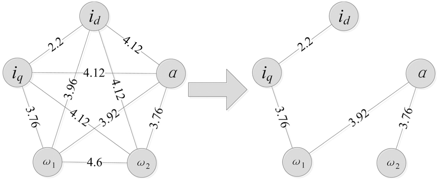
The optimized CPP analysis plane set of the system.

Principle of the chaotic phenomenon in the electromechanical coupling system

Chaos occurs in the dynamic trajectory of the electromechanical coupling system, and the system parameters are listed in Table 2. The principle of the chaotic trajectory was analyzed in the determined projection set P = {i_d-i_q, i_q-ω₁, ω₁-α, and ω₂-α}, then the dynamic characteristics can be revealed.

Table 2.

System parameters.

R₁ (Ω)	0.1	ψ_f (Wb)	0.63
L_d = L_q (H)	0.091	I₁ (kg m²)	0.041
I₂ (kg m²)	0.001	k (N/rad)	3e4
T_l (N m)	50	n_p	3
u_d (V)	380	u_q (V)	50

Substituting the value of variables in Table 2 into equation (7), characteristic roots are obtained: λ = (0.0006 + 5.5467i, 0.0006 − 5.5467i, −0.5488 + 1.0484i, −0.5488 − 1.0484i, 1.0989) × 10³. According to the five values of λ, there are three positive values. Therefore, the system is unstable. Thus, it must be analyzed by the CPP method.

1. The principle on the projection plane i_d-i_q

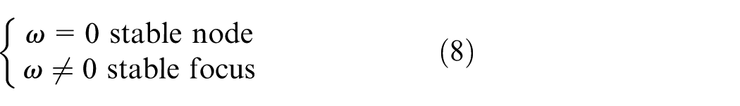
According to equation (8), when ω ≠ 0, the projection phase trajectory is at the stable focus state. Therefore, the phase trajectory on the projection plane i_d-i_q moves around the center point, which is the equilibrium. The equilibrium point moves along with the curve n_pω₁Li_q + u_d − R₁i_d = 0; therefore, the center point moves along with the curve n_pω₁Li_q +u_d − R₁i_d = 0.

According to the CPP analysis on the projection plane i_d-i_q, the equilibrium point moves along the curve n_pω₁Li_q + u_d − R₁i_d = 0. The equilibrium point is the stable node when ω₁ = 0, and the corresponding phase trajectory follows the stable node motion pattern. The equilibrium point is the stable focus point when ω ≠ 0, and the corresponding phase trajectory follows the stable focus point motion pattern. Figure 3 shows that during the whole time range, ω₁ ≠ 0, and the phase trajectory follows the stable focus point motion pattern. The phase trajectory’s center point moves with the equilibrium point. Figure 4(a) shows that the equilibrium point moves along with a line when t∈ (42,42.014), and therewith the phase trajectory’s center point. When the machine rotary speed ω₁ becomes larger, namely t∈ (82,82.004), ω₁ fluctuates, leading to the fluctuation of i_d and i_q. The phase trajectory’s center point did not move, since the equilibrium point fluctuates only slightly, as shown in Figure 4(b).

Figure 3.

t–ω₁ curve.

Figure 4.

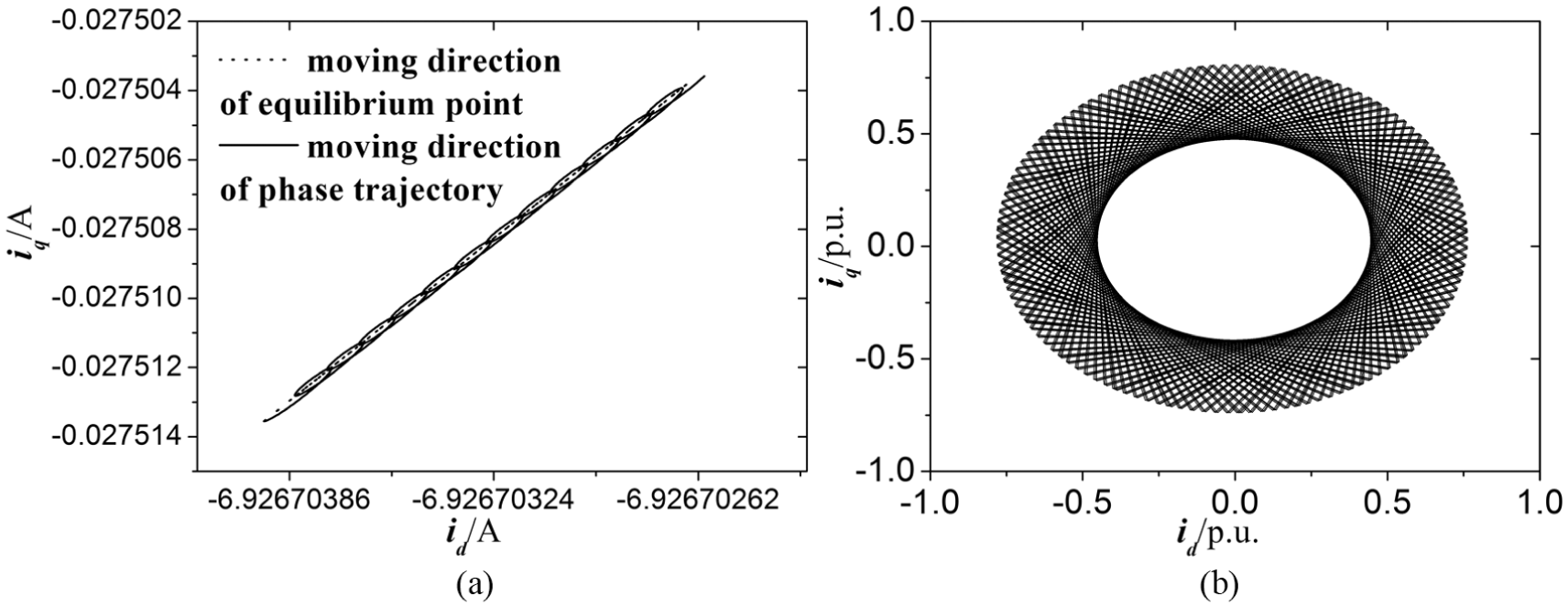
i_d-i_q phase trajectory: (a) t∈ (42,42.014) phase trajectory and (b) t∈ (82,82.004) phase trajectory.

2. The principle on the projection plane i_q-ω₁

On the projection plane i_q-ω₁, after a period of time, the phase trajectory moves following a circle, as shown in Figure 5.

Figure 5.

Phase trajectory on the projection plane i_q-ω_1.

According to the CPP analysis on the projection plane i_q-ω₁, the phase trajectory follows the saddle point motion pattern when i_d < −ψ_f/L and the stable node motion pattern when i_d > −ψ_f/L. Figure 6(a) shows that when t∈ (10,70), the phase trajectory moves away from the equilibrium point because i_d < −ψ_f/L during the period. Figure 6(b) shows that when t∈ (85,85.001), the phase trajectory switches between the saddle point motion pattern and the stable node motion pattern because i_q fluctuates on the point −ψ_f/L.

Figure 6.

Phase trajectory: (a) phase trajectory t∈ (10,70) and (b) phase trajectory t∈ (85,85.004).

3. The principle on the projection plane ω₁-α

Figure 7 shows that the phase trajectory of the projection plane ω₁-α follows a rotational motion.

Figure 7.

Phase trajectory on the projection plane ω₁-α.

According to the CPP analysis on the projection plane ω₁-α, the phase trajectory follows the center point motion pattern. Figure 8(a) shows the phase trajectory during t∈ (32,32.005). The phase trajectory’s rotary center moves, because the equilibrium point is on a horizontal line and then appears spiral as the equilibrium moves, and finally appears as a limiting circle, as shown in Figure 8(b).

Figure 8.

Phase trajectory: (a) phase trajectory during t∈ (32,32.005) and (b) phase trajectory during t∈ (85,85.005).

4. The principle on the projection plane ω₂-α

The phase trajectory is on the rotational motion on the projection plane ω₂-α, as shown in Figure 9.

Figure 9.

Phase trajectory on the projection plane ω₂-α.

According to the CPP analysis on the projection plane ω₁-α, the phase trajectory follows the center point motion pattern. Figure 10(a) shows the phase trajectory during t∈ (32,32.005). The phase trajectory’s rotary center moves because the equilibrium point is on a horizontal line and then appears spiral. During t∈ (85,85.005), the phase trajectory’s center moves as the equilibrium moves and then appears to be a limiting circle, as shown in Figure 10(b).

Figure 10.

Phase trajectory: (a) phase trajectory during t∈ (32,32.005) and (b) phase trajectory during t∈ (85,85.005).

Dynamic behavior analysis of the electromechanical coupling system

Using the CPP method, not only the dynamic behavior but also the special trajectory in a nonlinear system could be analyzed. The analysis on the projection plane set P = {i_d-i_q, i_q-ω₁, and ω₁-α, ω₂-α} shows that the bifurcation set structure and the moving rule of equilibrium on an arbitrary projection plane is relative to other state variables. The interaction between the five state variables forms the dynamic behavior of the electromechanical coupling system. The complexity of the projection subsystem is relatively small on the projection planes i_d-i_q and ω₂-α. Since the bifurcation set on the two projection planes has the state variable ω₁, the whole system’s dynamic behavior could be deduced by monitoring the range of ω₁ from the numerical integration.

Variable ω₁ converging at a constant C

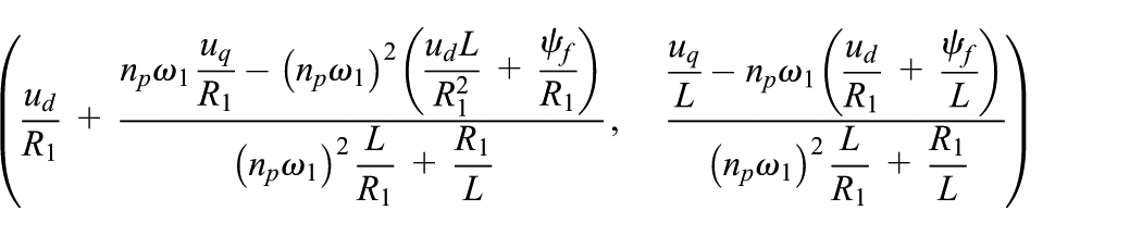
Since ω₁ = constant C, the phase trajectory on the projection plane i_d-i_q follows the stable node or stable focus motion pattern mode and finally converges at the equilibrium

\begin{matrix} {\frac{u_{d}}{R_{1}} + \frac{n_{p} ω_{1} \frac{u_{q}}{R_{1}} - {(n_{p} ω_{1})}^{2} (\frac{u_{d} L}{R_{1}^{2}} + \frac{ψ_{f}}{R_{1}})}{{(n_{p} ω_{1})}^{2} \frac{L}{R_{1}} + \frac{R_{1}}{L}}, \frac{\frac{u_{q}}{L} - n_{p} ω_{1} (\frac{u_{d}}{R_{1}} + \frac{ψ_{f}}{L})}{{(n_{p} ω_{1})}^{2} \frac{L}{R_{1}} + \frac{R_{1}}{L}}} \\ lim_{t \to \infty} i_{d} (t) = \frac{u_{d}}{R_{1}} + \frac{n_{p} ω_{1} \frac{u_{q}}{R_{1}} - {(n_{p} ω_{1})}^{2} (\frac{u_{d} L}{R_{1}^{2}} + \frac{ψ_{f}}{R_{1}})}{{(n_{p} ω_{1})}^{2} \frac{L}{R_{1}} + \frac{R_{1}}{L}}, lim_{t \to \infty} i_{q} (t) = \frac{\frac{u_{q}}{L} - n_{p} ω_{1} (\frac{u_{d}}{R_{1}} + \frac{ψ_{f}}{L})}{{(n_{p} ω_{1})}^{2} \frac{L}{R_{1}} + \frac{R_{1}}{L}} \end{matrix}

From the equation ${\overset{\cdot}{ω}}_{1} = (1 / I_{1}) (1.5 n_{p} ψ_{f} i_{q} - k α)$ , the following equation can be obtained: $lim_{t \to \infty} α (t) = (1.5 n_{p} ψ_{f} i_{q}) / k$ . Then, combining with the equation $\overset{\cdot}{α} = ω_{1} - ω_{2}$ , the following equation can be obtained: $lim_{t \to \infty} ω_{2} (t) = ω_{1}$ .

Above all, as long as the dynamic behavior of electromechanical coupling system satisfies ω₁ = constant C, the other state variables meet the following equations

lim_{t \to \infty} i_{d} (t) = \frac{u_{d}}{R_{1}} + \frac{n_{p} ω_{1} \frac{u_{q}}{R_{1}} - {(n_{p} ω_{1})}^{2} (\frac{u_{d} L}{R_{1}^{2}} + \frac{ψ_{f}}{R_{1}})}{{(n_{p} ω_{1})}^{2} \frac{L}{R_{1}} + \frac{R_{1}}{L}}

(9)

lim_{t \to \infty} i_{q} (t) = \frac{\frac{u_{q}}{L} - n_{p} ω_{1} (\frac{u_{d}}{R_{1}} + \frac{ψ_{f}}{L})}{{(n_{p} ω_{1})}^{2} \frac{L}{R_{1}} + \frac{R_{1}}{L}}

(10)

lim_{t \to \infty} α (t) = \frac{1.5 n_{p} ψ_{f} i_{q}}{k}

(11)

lim_{t \to \infty} ω_{2} (t) = ω_{1} = constant C

(12)

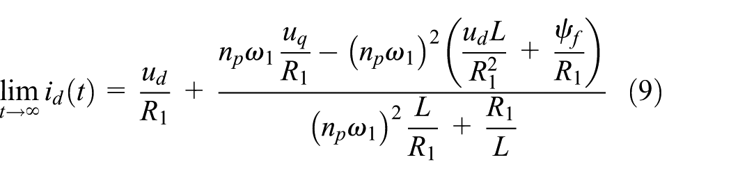
Figure 11 illustrates the simulation result with the system parameters. The data in Table 3 indicate that the system is stable.

Figure 11.

Simulation result of the system variables.

Table 3.

System parameters.

R₁ (Ω)	6.1	ψ_f (Wb)	0.63
L_d = L_q (H)	0.011	I₁ (kg m²)	0.001
I₂ (kg m²)	0.081	K (N/rad)	6e4
T_l (N m)	50	n_p	3
u_d (V)	191	u_q (V)	50

Substituting the value of variables in Table 3 to equation (7), characteristic roots were obtained: λ = (−6.7028 + 0.0677i, −6.7028 − 0.0677i, −0.0003 + 0.0442i, −0.0003 − 0.0442i, −0.0003) × 10⁴. The real parts of λ are all negative values. Therefore, the system is stable, and it is also proved, as shown in Figure 11.

Variable ω₁ fluctuating the constant C

If the value of ω₁ fluctuates, the phase trajectory on the projection plane follows the center point motion pattern. Moreover, the trajectory center point fluctuates with ω₁. Thereby, the 5-DOF system could form the helical trajectory, finally leading to chaos.

Results and discussion

In this section, the CPP method is presented to reduce the 5-DOF system to the 2-DOF system. In order to complete the system, the dynamic characteristics of four projection planes were analyzed, when the other three variables change. Moreover, the complexity of the projection subsystem is relatively small on the projection planes i_d-i_q and ω₂-α. Since the bifurcation set on the two projection planes has the state variable ω₁, the dynamic behavior of whole system could be deduced by monitoring the range of ω₁ from the numerical integration. Therefore, the dynamic stability of the two projective planes was analyzed when the value of ω₁ tends to be stable and fluctuate. Moreover, the results of this study show that the electromechanical system will be stable if the ω₁ value is controlled in a stable area.

Conclusion

In conclusion, the electromechanical coupling system was investigated using a 5-DOF dynamic model. The stability of the model was studied, considering the effect of electromechanical coupling. Because the model which contains the nonlinear characteristics is large, the CPP method was used to reduce the system’s number of 5-DOF to 2-DOF. The theory of nonlinear stability was applied to analyze the system. The following conclusions were drawn:

In this study, four coordinate planes, i_d-i_q, i_q-ω₁, ω₁-α, and α-ω₂ planes, were chosen to reflect the original 5-DOF electromechanical system. On the plane i_d-i_q, the phase trajectory may converse from the stable state to the limit cycle moving state when the variable ω₁ fluctuates; on the plane i_q-ω₁, the moving pattern varies along with the variable i_q; on the plane ω₁-α, different patterns of the manifestation of the center point moving pattern were analyzed; on the plane α-ω₂, different patterns of the manifestation of the center point moving pattern during different periods were analyzed. This analysis concludes that the four projection planes could reflect the characteristics of the original 5-DOF system.

Through the characteristic analysis of the coordinate plane and the electromechanical coupling equation, using ω₁ as the known parameter, the moving pattern of the i_d-i_q and α-ω₂ subsystems were determined. Namely, if the variable ω₁ tends to be a constant, then the other four variables tend to be constant; if the variable ω₁ holds wave nearby a constant, the other four state variables are not stable. Thus, the electromechanical coupling system can be fully controlled by only controlling the ω₁ variable.

The system will exhibit a helical trajectory if the rotational speed of the PMSM is unstable; the system will exhibit stable behavior if the rotational speed of the PMSM is going to be stable. Therefore, parameters were chosen to stabilize the rotational speed of the PMSM in order for the coupling system to exhibit a stable behavior.

This study used the CPP method, which is only used in the power system up to now. Through this CPP method, the 5-DOF system was successfully reduced to a 2-DOF system. Moreover, the conditions under which the coupling system exhibits specific behavior are presented. Extending this study to the control area has a large scope. Some control strategies for the electromechanical coupling system could be built to avoid or utilize the chaos of the system.

Footnotes

Appendix 1

The equations of the 10 planes in section “Analysis of the electromechanical 5-DOF system using CPP method” are as follows

(13)

{\begin{matrix} {\overset{\cdot}{i}}_{d} = \frac{u_{d}}{L} + n_{p} ω_{1} i_{q} - \frac{1}{L} R_{1} i_{d} \\ {\overset{\cdot}{i}}_{q} = \frac{u_{q}}{L} - n_{p} ω_{1} i_{d} - n_{p} ω_{1} \frac{ψ_{f}}{L} - \frac{1}{L} R_{1} i_{q} \end{matrix}

(14)

{\begin{matrix} {\overset{\cdot}{i}}_{d} = \frac{u_{d}}{L} + n_{p} ω_{1} i_{q} - \frac{1}{L} R_{1} i_{d} \\ {\overset{\cdot}{ω}}_{1} = \frac{1}{I_{1}} (1.5 n_{p} ψ_{f} i_{q} - k α) \end{matrix}

(15)

{\begin{matrix} {\overset{\cdot}{i}}_{d} = \frac{u_{d}}{L} + n_{p} ω_{1} i_{q} - \frac{1}{L} R_{1} i_{d} \\ {\overset{\cdot}{ω}}_{2} = \frac{1}{I_{2}} (k α - T_{l}) \end{matrix}

(16)

{\begin{matrix} {\overset{\cdot}{i}}_{d} = \frac{u_{d}}{L} + n_{p} ω_{1} i_{q} - \frac{1}{L} R_{1} i_{d} \\ \overset{\cdot}{α} = ω_{1} - ω_{2} \end{matrix}

(17)

{\begin{matrix} {\overset{\cdot}{i}}_{q} = \frac{u_{q}}{L} - n_{p} ω_{1} i_{d} - n_{p} ω_{1} \frac{ψ_{f}}{L} - \frac{1}{L} R_{1} i_{q} \\ {\overset{\cdot}{ω}}_{1} = \frac{1}{I_{1}} (1.5 n_{p} ψ_{f} i_{q} - k α) \end{matrix}

(18)

{\begin{matrix} i_{d} < - \frac{ψ_{f}}{L} saddle point \\ i_{d} > - \frac{ψ_{f}}{L} stable node \end{matrix}

(19)

{\begin{matrix} {\overset{\cdot}{i}}_{q} = \frac{u_{q}}{L} - n_{p} ω_{1} i_{d} - n_{p} ω_{1} \frac{ψ_{f}}{L} - \frac{1}{L} R_{1} i_{q} \\ {\overset{\cdot}{ω}}_{2} = \frac{1}{I_{2}} (k α - T_{l}) \end{matrix}

(20)

{\begin{matrix} {\overset{\cdot}{i}}_{q} = \frac{u_{q}}{L} - n_{p} ω_{1} i_{d} - n_{p} ω_{1} \frac{ψ_{f}}{L} - \frac{1}{L} R_{1} i_{q} \\ \overset{\cdot}{α} = ω_{1} - ω_{2} \end{matrix}

(21)

{\begin{matrix} {\overset{\cdot}{ω}}_{1} = \frac{1}{I_{1}} (1.5 n_{p} ψ_{f} i_{q} - k α) \\ {\overset{\cdot}{ω}}_{2} = \frac{1}{I_{2}} (k α - T_{l}) \end{matrix}

(22)

{\begin{matrix} {\overset{\cdot}{ω}}_{1} = \frac{1}{I_{1}} (1.5 n_{p} ψ_{f} i_{q} - k α) \\ \overset{\cdot}{α} = ω_{1} - ω_{2} \end{matrix}

(23)

{\begin{matrix} {\overset{\cdot}{ω}}_{2} = \frac{1}{I_{2}} (k α - T_{l}) \\ \overset{\cdot}{α} = ω_{1} - ω_{2} \end{matrix}

Academic Editor: Francesco Massi

Declaration of conflicting interests

The author(s) declared no potential conflicts of interest with respect to the research, authorship, and/or publication of this article.

Funding

The author(s) disclosed receipt of the following financial support for the research, authorship, and/or publication of this article: This study was supported by the National Natural Science Foundation of China (NSFC; 51305032).

References

Gao

Chen

Tan

. Application of chaos in permanent-magnet synchronous motor optimization. Appl Mech Mater 2013; 385: 1147–1150.

Meng

Zhang

W-M

Huang

. Micro-rotor dynamics for micro-electro-mechanical systems (MEMS). Chaos Solit Fract 2009; 40: 538–562.

Darula

Sorokin

. On non-linear dynamics of a coupled electro-mechanical system. Nonlinear Dynam 2012; 70: 979–998.

Confalonieri

Corigliano

Dossi

. A domain decomposition technique applied to the solution of coupled electro-mechanical problem. Int J Numer Meth Eng 2013; 93: 137–159.

Coria

Starkov

. Bounding a domain containing all compact invariant sets of the permanent-magnet motor system. Commun Nonlinear Sci 2009; 14: 3879–3888.

Zhang

Kong

H-Y

. Self-sustained oscillation and harmonic generation in optomechanical systems with quadratic couplings. Phys Rev A 2014; 89: 1–10.

Schroder

. Derivation of the localization and homogenization conditions for electro-mechanically coupled problems. Comput Mater Sci 2009; 46: 593–599.

Meyk

. Minimization of transient forces in an electro-mechanical system. Struct Multidiscip O 1994; 8: 251–256.

Yao

Hikihara

. Counter operation in nonlinear micro-electro-mechanical resonators. Phys Lett A 2013; 377: 2551–2555.

10.

Xue

. The stability-preserving trajectory-reduction methodology for analyzing nonlinear dynamics (keynote). In: Proceedings of the international conferences on info-net (IEEE catalog number: 01EX497), vol. 4, Beijing, China, 29 October 2001, pp.7–19. New York: IEEE.

11.

Shao

Z-G

. The dynamic analysis of power system and other general dynamic system. Nanjing, China: Southeast University, 2004.

12.

Park

Joo

. Bifurcations and chaos in a permanent-magnet synchronous motor. IEEE T Circuits: I 2002; 49: 383–387.

13.

Jing

Chen

. Complex dynamics in a permanent-magnet synchronous motor model. Chaos Solit Fract 2004; 22: 831–848.

14.

Hemati

Kwatny

. Bifurcation of equilibria and chaos in permanent-magnet machines. In: Proceedings of the 32nd IEEE conference on decision and control, San Antonio, TX, 15–17 December 1993, pp.475–479. New York: IEEE.

15.

Zaher

. A nonlinear controller design for PM motors using a synchronization-based technique inspired from the Lorenz system. Chaos 2008; 18: 174–188.

16.

Liu

Zhao

S-S

Sun

B-P

. Bifurcation and chaos analysis of a nonlinear electromechanical coupling relative rotation systems. Chinese Phys B 2014; 23: 271–277.

17.

Wei

Zhang

Luo

. Effects of couplings on the collective dynamics of permanent-magnet synchronous motors. IEEE T Circuits: II 2013; 60: 692–696.

18.

Niu

Qiu

. Investigation of torsional instability, bifurcation, and chaos of a generator set. IEEE T Energy Conver 2002; 17: 164–168.

19.

Park

. Two-reaction theory of synchronous machines: generalized method of analysis—part I. Trans Am Inst Electr Eng 1929; 48: 716–727.

20.

Park

. Two-reaction theory of synchronous machines—part II. Electr Eng 1933; 52: 44–45.

Analysis of torsional stability and the dynamical characteristics of electromechanical systems

Abstract

Keywords

Introduction

Model and equations

Dynamic behaviors of the electromechanical coupling system

Analysis of the electromechanical 5-DOF system using CPP method

Projection plane set of the electromechanical coupling system

Principle of the chaotic phenomenon in the electromechanical coupling system

Dynamic behavior analysis of the electromechanical coupling system

Variable ω1 converging at a constant C

Variable ω1 fluctuating the constant C

Results and discussion

Conclusion

Footnotes

Appendix 1

Declaration of conflicting interests

Funding

References

Variable ω₁ converging at a constant C

Variable ω₁ fluctuating the constant C