Sage Journals: Discover world-class research

Abstract

The thermal performance of a building refers to the process of modeling the energy transfer between a building and its surroundings. The objective of this work is to develop a new correlation to estimate the number of Nusselt predictions, to facilitate the design of the walls of buildings based on a numerical simulation with a computational fluid dynamics software which can be coupled after with the Lagrange polynomial interpolation method for high Rayleigh number. For this purpose, a building is modeled as a collection of basic elements (walls, rooms, etc.). Moreover, we developed a FORTRAN program to control the equation of high order. This method is for predicting exchange coefficient and estimating Nusselt number of convection to optimize the design of walls in buildings. This method was performed via the simulation and theoretical case.

Keywords

Building material heat transfer in building natural convection polynomial interpolation method thermal environment wall design

Introduction

The thermophysical properties of the building envelope have been identified as key parameters in the determination and explanation of the energy performance of buildings and are widely used in models to predict the energy demand of the built stock.^1–4 The thermal building is a real problem in Algeria. In the world, 40% is the amount of energy consumed in the construction^5,6 and, in turn, supports 23%–40% of the world’s greenhouse gas emission, particularly CO₂.⁷ Several works have been published in this direction and in several newspapers and journals such as Building Engineering Building and Environment,⁸Building and Environment,^9–11Energy Storage,^12–16 and Energy and Buildings.^17–29 In most situations, the mechanical cooling devices offer solutions that are neither environment friendly nor energy sustainable. The mechanical devices are non-functional and cannot offer thermal comfort without energy input. Hence, utilization of advanced building materials and passive technologies in buildings may offer the solution for thermal comfort demands, substantially reduce the energy demand, and impact on the environment and carbon footprint of building stock worldwide.³⁰ Also, numerous studies across the world have shown the impacts of hot working environments on the working population.^31–39 Furthermore, over the last few decades, the interest around phase change materials (PCM) was regarded as a possible solution into building structures. Even though the use of PCM in the envelope can minimize heating and cooling loads, the good design of the walls of the houses remains the most important keys to conserve energy, especially with the recent turmoil in the global oil markets. First, in this article, computational fluid dynamics (CFD) software is used as a technique to modeling the behavior of fluid and the thermal convection in the external wall of the house with different Rayleigh numbers. Second, the fundamental idea in this work is to vary the thickness of the building material of the outer wall four times and calculate the Nusselt number and exchange coefficient of heat transfer to find a cloud point, respectively, for the thicknesses e = 0, L/40, L/20, and L/10. Afterward, we developed a relationship that helps us to know the exchange ratio for each thickness e belongs to the interval [0, L/10] by the Lagrange polynomial interpolation method and then we developed a FORTRAN program to control this equation. This method is for predicting exchange coefficient of convection to optimize the design of walls in buildings before starting the wall construction for Rayleigh number equal to 10⁵.

Geometric configuration

To solve this problem, the fluid is considered Newtonian and incompressible and the approximation of Boussinesq is presented. In addition, viscous friction is neglected. The dimensions of the design are as follows: H = 1, L = 1 T_c = 1, T_f = 0, and the aspect ratio A = 1. We consider the concrete wall with the following properties:

Density (ρ): 2200 kg/m³;

Thermal conductivity (λ): 1.75 W/(m K);

Specific heat (Cp): 878 J/(kg K).

Objectives

The most important point in this work is to present the prediction of the wall design through numerical evaluation of the convection in buildings by the Lagrange polynomial interpolation method, as well as to present the modeling study of the conduction convection coupling.

Mathematical modeling

The governing equations can be given by:

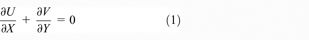
Continuity equation

\frac{\partial U}{\partial X} + \frac{\partial V}{\partial Y} = 0

(1)

X-momentum equation

\frac{\partial U}{\partial t} + U \frac{\partial U}{\partial X} + V \frac{\partial U}{\partial Y} = - \frac{1}{ρ} \frac{\partial P}{\partial X} + υ \nabla^{2} U

(2)

Y-momentum equation

\frac{\partial V}{\partial t} + U \frac{\partial V}{\partial X} + V \frac{\partial V}{\partial Y} = - \frac{1}{ρ} \frac{\partial P}{\partial X} + υ \nabla^{2} V + g β \frac{\partial T}{\partial X}

(3)

Energy equation

\frac{\partial T}{\partial t} + U \frac{\partial T}{\partial X} + V \frac{\partial T}{\partial Y} = \frac{λ}{ρ c_{p}} \nabla^{2} T + \frac{1}{ρ c_{p}} φ

(4)

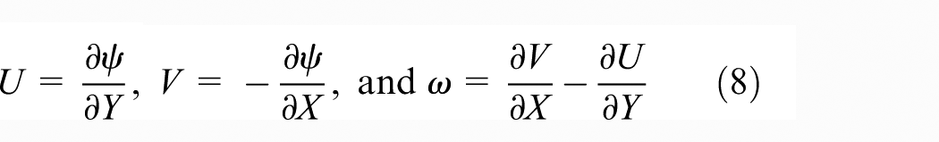
The derived equation (2) over Y and the equation (3) over X after subtracting the two equations are obtained. The equations dimensionless variables in writing Helmotz in terms of vorticity and stream function formulation are given by

\frac{\partial ω}{\partial t} + U \frac{\partial ω}{\partial X} + V \frac{\partial ω}{\partial Y} = \Pr \nabla^{2} ω + Ra \Pr \frac{\partial T}{\partial X}

(5)

\frac{\partial θ}{\partial t} + U \frac{\partial T}{\partial X} + V \frac{\partial T}{\partial Y} = \frac{\partial^{2} T}{\partial X^{2}} + \frac{\partial^{2} T}{\partial Y^{2}} + \frac{φ}{ρ Cp} \frac{L^{2}}{a Δ T}

(6)

\frac{\partial^{2} ψ}{\partial X^{2}} + \frac{\partial^{2} ψ}{\partial Y^{2}} = - ω

(7)

U = \frac{\partial ψ}{\partial Y}, V = - \frac{\partial ψ}{\partial X}, and ω = \frac{\partial V}{\partial X} - \frac{\partial U}{\partial Y}

(8)

Using the dimensionless variables in the equations above are defined by

{\begin{matrix} X^{*} = \frac{x}{L}, Y^{*} = \frac{y}{L}, U^{*} = \frac{u}{u_{i}} \\ V^{*} = \frac{ν}{u_{i}}, P^{*} = \frac{P}{ρ u_{i}^{2}}, T * = \frac{T - T_{i}}{T_{c} - T_{i}}, t * = \frac{t}{L^{2} / a} \end{matrix}

(9)

For the concrete, the energy equation is given by

\frac{\partial T}{\partial t} = \frac{1}{a} (\frac{\partial^{2} T}{\partial X^{2}} + \frac{\partial^{2} T}{\partial Y^{2}})

(10)

Procedure of simulation

First, the GAMBIT and FLUENT softwares are used for this numerical simulation. For the convection terms, a first order of Apwind scheme, also simple algorithm,⁴⁰ is used to couple momentum and continuity equations. The convergence between two successive times is not less than 1e4. With an aim of following well any variation of the thermal and hydrodynamic fields, we used a uniform grid of 14,480 elements and 14,241 nodes in non-stationary mode. Second, we developed a FORTRAN program to control the linear equation of order three. We assume that the flow and heat transfer are two-dimensional and the physical properties of air are constant and the Boussinesq approximation is validated. The boundary condition and physical parameters are defined as follows: H = 1, L = 1 T_c = 1, T_f = 0, and the aspect ratio A = 1. We consider concrete wall.

Validation

For the validation of the model, we compared our results with those obtained by De Vahl Davis⁴¹ (see Table 1).

Table 1.

Comparisons of the results of validation.

	$\bar{Nu}$
	Present	De Vahl Davis⁴¹	Error
Ra = 10³	1.2	1.12	0.08
Ra = 10⁴	2.257	2.243	0.014
Ra = 10⁵	4.64	4.52	0.12

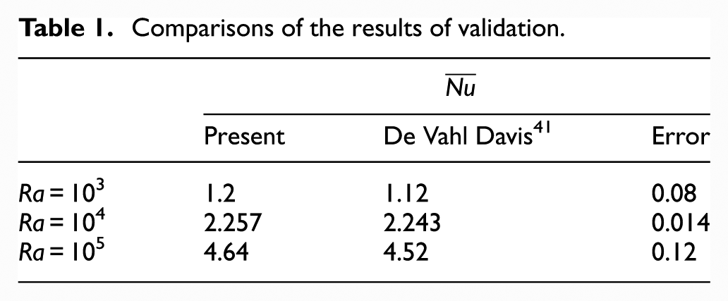
First, the natural convection model is validated against a benchmark: a differentially heated square cavity with adiabatic horizontal walls and constant temperature vertical walls, as described by De Val Devis,⁴¹ the case that is adapted to our proposition, where the wall thickness is equal to e = 0.

Mathematical model for the Lagrange polynomial interpolation method

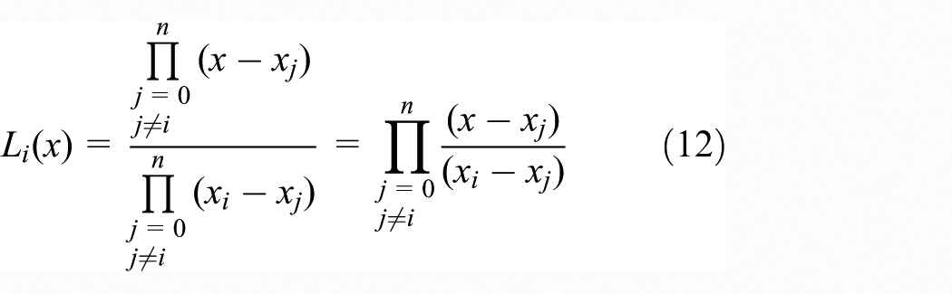
The Lagrange interpolating polynomial is the polynomial of degree ≤(N − 1) that passes through the n points (x₁, y₁), (x₂, y₂), …, (x_n, y_n), and the interpolation polynomial in the Lagrange form is a linear combination and is given by

P_{n} (x) = \sum_{i = 0}^{n} y_{i} L_{i} (x)

(11)

For Lagrange basis polynomials

L_{i} (x) = \frac{Π_{\binom{j = 0}{j \neq i}}^{n} (x - x_{j})}{Π_{\binom{j = 0}{j \neq i}}^{n} (x_{i} - x_{j})} = Π_{\binom{j = 0}{j \neq i}}^{n} \frac{(x - x_{j})}{(x_{i} - x_{j})}

(12)

where

{\begin{matrix} L_{i} (x_{j}) = 0 & if & i \neq j \\ L_{i} (x_{j}) = 1 & if & i = j \end{matrix}

(13)

The polynomial interpolation points

We wish to find the polynomial interpolating the points (Table 2).

Table 2.

The sets of polynomial interpolation points.

	B = e/L	$\bar{Nu}$
Ra = 10⁵	0	4.50
	1/40	3.77
	1/20	3.12
	1/10	2.20

The points of Nu(e) are obtained by numerical simulation of the FLUENT software, for the Rayleigh number equal to 10⁵.

The error estimates

The question that we consider here is: how accurately does the polynomial p_n(x) approximate the function f(x) at any point x?

So, let f∈C[a; b], (n + 1) differentiable on (a; b) and let x₀; x₁; x₂; …; x_n be (n + 1) distinct points in [a; b]. If p_n(x) is such that p_n(x_i) = f(x_i); i = 0; 1; …; n, then for each x∈[a; b] there exists ε(x) ∈ [a; b] such that

E_{N} (x) = f (x) - p_{n} (x) = \frac{f^{n + 1} ε (x)}{(n + 1)!} Π_{i = 0}^{n} (x - x_{i})

(14)

where E_N(x) is the error in the approximation of f(x).

Results and discussion

The boundary conditions have been established to simulate a geometric configuration used frequently in two-dimensional approximation (Figure 1).

Figure 1.

The geometry considered.

Isotherms

The isotherms are presented in Figure 2. Gradually, as the Rayleigh number increases, the isotherms become increasingly wavy and heat transfer increases, so the flow intensifies and natural convection is expanding and predominates.

Figure 2.

The isotherms for wall thickness e = L/20 and for different Rayleigh numbers, Pr = 0.71.

Lagrange polynomials

The points of Nu(e) are obtained by numerical simulation of the FLUENT software, for the Rayleigh number equal to 10⁵ (see Table 3).

Table 3.

Nusselt number for different values of thickness and for Ra = 10⁵.

	i	X_i = e	$Y_{i} = \bar{Nu} (e)$
Ra = 10⁵	0	0	4.50
Ra = 10⁵	1	e = L/40	3.77
Ra = 10⁵	2	e = L/20	3.12
Ra = 10⁵	3	e = L/10	2.20

If (0, 4.50), (L/40, 3.77), (L/20, 3.12), and (L/10, 2.20) are given data points, then the cubic polynomial passing through these points can be expressed as

P_{3} (x) = y_{0} l_{0} + y_{1} l_{1} + y_{2} l_{2} + y_{3} l_{3}

We would have the four basis polynomials

L_{0} = \frac{(x - \frac{L}{40}) (x - \frac{L}{20}) (x - \frac{L}{10})}{(0 - \frac{L}{40}) (0 - \frac{L}{20}) (0 - \frac{L}{10})}

(15)

L_{1} = \frac{(x - 0) (x - \frac{L}{20}) (x - \frac{L}{10})}{(\frac{L}{40} - 0) (\frac{L}{40} - \frac{L}{20}) (\frac{L}{40} - \frac{L}{10})}

(16)

L_{2} = \frac{(x - 0) (x - \frac{L}{40}) (x - \frac{L}{10})}{(\frac{L}{20} - 0) (\frac{L}{20} - \frac{L}{40}) (\frac{L}{20} - \frac{L}{10})}

(17)

L_{3} = \frac{(x - 0) (x - \frac{L}{40}) (x - \frac{L}{20})}{(\frac{L}{10} - 0) (\frac{L}{10} - \frac{L}{40}) (\frac{L}{10} - \frac{L}{20})}

(18)

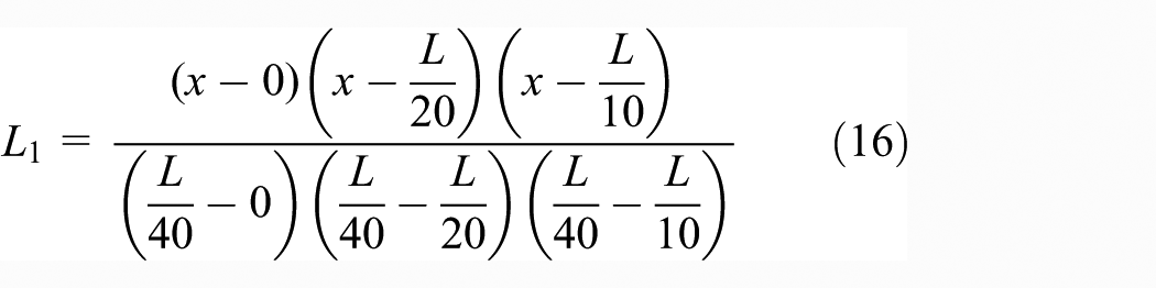
The polynomial P(x) given by the above formula is called Lagrange’s interpolating polynomial and the functions (15)–(18) are called Lagrange’s interpolating basis functions.

Nusselt number correlations

It should be noted that the numerical result is given by equation (21). Remarkably, similar to the estimate of the average Nusselt number by the Lagrange interpolation method for each wall thickness between [0, L/10] but only for Ra = 10⁵

P_{3} (x) = y_{0} l_{0} + y_{1} l_{1} + y_{2} l_{2} + y_{3} l_{3}

(19)

P_{3} (x) = 4.5 l_{0} + 3.77 l_{1} + 3.12 l_{2} + 2.20 l_{3}

(20)

P_{3} (x) = - \frac{1120}{3 L^{3}} x^{3} + \frac{36}{L^{2}} x^{2} - \frac{30.33}{L} x + 4.5

(21)

Therefore, we can write

\bar{Nu} (e) = - \frac{373.33}{L^{3}} e^{3} + \frac{36}{L^{2}} e^{2} - \frac{30.33}{L} e + 4.5

(22)

where $\bar{Nu}$ is the average Nusselt number and e is wall thickness.

Also, we can write

\bar{Nu} = - 373.33 B^{3} + 36 B^{2} - 30.33 B + 4.5

(23)

where B: e/L.

In heat transfer, the average Nusselt number is given by

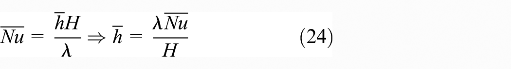
\bar{Nu} = \frac{\bar{h} H}{λ} \Rightarrow \bar{h} = \frac{λ \bar{Nu}}{H}

(24)

where H is the characteristic length, λ is the thermal conductivity of the fluid, and $\bar{h}$ is the convective heat transfer coefficient of the flow.

Average Nusselt numbers

The decrease in Nusselt number is more as shown in Figure 3 with increase in the wall thickness, and the heat transfer also decreases because the inertia and the thermal resistance of the wall increase. Also, the increase in Nusselt number is more as shown in Figure 4. Broadly, advection becomes stronger and thus heat transfer increases.

Figure 3.

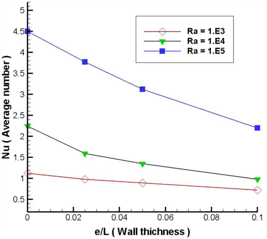
Average Nusselt number profiles for different wall thicknesses and for different Rayleigh numbers, Ra = 10³, 10⁴, and 10⁵ and Pr = 0.71.

Figure 4.

Profiles of average Nusselt number for different Rayleigh numbers, Ra = 10³, 10⁴, and 10⁵ and Pr = 0.71.

Conclusion

Thermal comfort has a significant value in this work for 10³ ≤ Ra ≤ 10⁵ and Pr = 0.71. Concrete wall for different thicknesses is viewed with 0 ≤ e ≤ L/10. We are interested in convection conduction coupling. First, CFD software is used as a technique to modeling the behavior of fluid and the thermal convection in the external wall of the house. Second, the most important part in this work is to vary the thickness of the building material of the outer wall four times and calculate the Nusselt number and exchange coefficient of heat transfer to find a cloud point, respectively, for the thicknesses e = 0, L/40, L/20, and L/10. Afterward, we developed a relationship that helps us to know the Nusselt number and exchange ratio for each thickness (e) belongs to the interval [0, L/10] by the Lagrange polynomial interpolation method and then we developed a FORTRAN program to control the nonlinear equation of order three (equation (22) or equation (23)). This method is for predicting exchange coefficient of convection to optimize the design of walls in buildings. Since, in interpolation we must determine a mathematical equation include and pass on a set of points, predictive simple correlation was developed to estimate the value of the average Nusselt number and the coefficient of heat transfer for exchange any thickness ranging from 0 to L/10. It is just enough to replace the thickness value in equation (21), to calculate the Nusselt number planned before the design and construction of walls.

Footnotes

Acknowledgements

The authors thank all reviewers for taking the time and energy to review our work.

Academic Editor: Yanping Yuan

Declaration of conflicting interests

The author(s) declared no potential conflicts of interest with respect to the research, authorship, and/or publication of this article.

Funding

The author(s) disclosed receipt of the following financial support for the research, authorship, and/or publication of this article: This work was supported by the Research program sponsored by the Faculty of Science and Technology, Department of technology, ENERGARID Laboratory, T.M. University, Bechar, Algeria.

References

Gori

Marincioni

Biddulph

. Inferring the thermal resistance and effective thermal mass distribution of a wall from in situ measurements to characterise heat transfer at both the interior and exterior surfaces. Energ Buildings 2017; 135: 398–409.

Hughes

Palmer

Cheng

. Global sensitivity analysis of England’s housing energy model. J Build Perform Simul 2015; 8: 283–294.

Stone

Shipworth

Biddulph

. Key factors determining the energy rating of existing English houses. Build Res Inf 2014; 42: 725–738.

De Wit

. Uncertainty in building simulation. In: Malkawi

Augenbroe

(eds) Advanced building simulation. Abingdon: Taylor & Francis, 2004, pp.25–59.

Zhang

Cooke

. Green building and energy efficiency. Cardiff: Center for Advanced Studies, Cardiff University, 2012.

Olukoya Obafemi

Kurt

. Environmental impacts of adobe as a building material: the north cyprus traditional building case. Case Stud Constr Mater 2016; 4: 32–41.

Gunnell

Chrisna

Gibberd

. Green building in South Africa: emerging trends. Pretoria: Department of Environmental Affairs and Tourism, The Republic of South Africa, 2009.

Galvin

. How many interviews are enough? Do qualitative interviews in building energy consumption research produce reliable knowledge? J Build Eng 2015; 1: 2–12.

Seon Park

Hong

. Methodology for assessing human health impacts due to pollutants emitted from building materials. Build Environ 2016; 95: 133–144.

10.

Tsapalov

Kovler

. Revisiting the concept for evaluation of radon protective properties of building insulation materials. Build Environ 2016; 95: 182–188.

11.

Lyng

Gunnarsen

Andersen

. Measurement of PCB emissions from building surfaces using a novel portable emission test cell. Build Environ 2016; 101: 77–84.

12.

Thambidurai

Panchabikesan

Krishna Mohan

. Review on phase change material based free cooling of buildings—the way toward sustainability. J Energ Storage 2015; 4: 74–88.

13.

Heinrich Badenhorst

Sandrock

. Novel method for thermal conductivity measurement through flux signal deconvolution. J Energ Storage 2016; 6: 32–39.

14.

Bader

Ouederni

. Optimization of biomass-based carbon materials for hydrogen storage. J Energ Storage 2016; 5: 77–84.

15.

Elsayed

. Numerical study on performance enhancement of solid–solid phase change materials by using multi-nanoparticles mixtures. J Energ Storage 2015; 4: 106–112.

16.

Singh

Dhiman

. Exergoeconomic analysis of recyclic packed bed solar air heater-sustained air heating system for buildings. J Energ Storage 2016; 5: 33–47.

17.

Chiang

Natarajan

Walker

. A laboratory test of the efficacy of energy display interface design. Energy Build 2012; 55: 471–480.

18.

Coleman

Brown

Wright

. Information, communication and entertainment appliance use—insights from a UK household study. Energy Build 2012; 54: 61–72.

19.

Galvin

. Impediments to energy-efficient ventilation of German dwellings: a case study in Aachen. Energy Build 2013; 56: 32–40.

20.

Gram-Hanssen

Christensen

Petersen

. Air-to-air heat pumps in real-life use: are potential savings achieved or are they transformed into increased comfort? Energy Build 2012; 53: 64–73.

21.

Jovanovíc

Pejíc

Djoríc-Veljkovíc

. Importance of building orientation in determining daylighting quality in student dorm rooms: physical and simulated daylighting parameters’ values compared to subjective survey results. Energy Build 2014; 77: 158–170.

22.

Kanters

Horvat

Dubois

. Tools and methods used by architects for solar design. Energy Build 2014; 68: 721–731.

23.

Santamouris

Alevizos

Aslanoglou

. Freezing the poor—indoor environmental quality in low and very low income households during the winter period in Athens. Energy Build 2014; 70: 61–70.

24.

Karjalainen

. Consumer preferences for feedback on household electricity consumption. Energy Build 2011; 43: 458–467.

25.

Karjalainen

. Should it be automatic or manual—the occupant’s perspective on the design of domestic control systems. Energy Build 2013; 65: 119–126.

26.

Menzies

Wherrett

. Windows in the workplace: examining issues of environmental sustainability and occupant comfort in the selection of multi-glazed windows. Energy Build 2005; 37: 623–630.

27.

Ridley

Bere

Clark

. The side by side in use monitored performance of two passive and low carbon Welsh houses. Energy Build 2014; 82: 13–26.

28.

Risholt

Time

Hestnes

. Sustainability assessment of nearly zero energy renovation of dwellings based on energy, economy and home quality indicators. Energy Build 2013; 60: 217–224.

29.

Sookchaiy

Monyakul

Thep

. Assessment of the thermal environment effects on human comfort and health for the development of novel air conditioning system in tropical regions. Energy Build 2010; 42: 1692–1702.

30.

Latha

Darshana

Vidhya

. Role of building material in thermal comfort in tropical climates—a review. J Build Eng 2015; 3: 104–113.

31.

Arngrïmsson

Petitt

Stueck

. Cooling vest worn during active warm-up improves 5-km run performance in the heat. J Appl Physiol 2004; 96: 1867–1874.

32.

González-Alonso

Ceandall

Johnson

. The cardiovascular challenge of exercising in the heat. J Physiol 2008; 586: 45–53.

33.

Wesseling

Crowe

Hogstedt

. Resolving the enigma of the Mesoamerican nephropathy: a research workshop summary. Am J Kidney Dis2014; 63: 396–404.

34.

Bridger

. Introduction to ergonomics. 2nd ed.London: Taylor & Francis, 2003, p. 780.

35.

Bates

Schneider

. Hydration status and physiological workload of UAE construction workers: a prospective longitudinal observational study. J Occup Med Toxicol 2008; 3: 21–26.

36.

Dutta

Chorsiya

. Scenario of climate change and human health in India. Int J Innov Res Dev 2013; 2: 157–160.

37.

Benachour

Draoui

Imine

. Study of the influence of the mural heating on the convection in the building in arid area. Int Rev Mech Eng 2015; 9: 476–481.

38.

Benachour

Draoui

Rahmani

. Effect of positioning the heating element on natural convection in square cavity (habitat type). Int Rev Mech Eng 2010; 4: 476–481.

39.

Benachour

Belkacem

Khadidja

. Numerical simulation of the influence of external insulation by the mud on the convection in the buildings. In: Proceedings of the 3rd international conference on fluid flow, heat and mass transfer (FFHMT’16), Ottawa, ON, Canada, 2–3 May 2016, paper no. 127.

40.

Patankar

. Numerical heat transfer and fluid flow. New York: McGraw-Hill Education, 1980.

41.

De Vahl Davis

. Natural convection of air in a square cavity: a bench mark numerical solution. Int J Numer Meth Fl 1983; 3: 249–264.

Numerical simulation of conjugate convection combined with the thermal conduction using a polynomial interpolation method

Abstract

Keywords

Introduction

Geometric configuration

Objectives

Mathematical modeling

Procedure of simulation

Validation

Mathematical model for the Lagrange polynomial interpolation method

The polynomial interpolation points

The error estimates

Results and discussion

Isotherms

Lagrange polynomials

Nusselt number correlations

Average Nusselt numbers

Conclusion

Footnotes

Acknowledgements

Declaration of conflicting interests

Funding

References