
Abstract
Through combined experimental and finite element analysis, the effect of bulk compressibility on rubber isolators was studied. First, the strain energy functions for rubber materials were studied, and the volumetric term was described by Poisson’s ratio. Second, parameter identification tests of rubber specimens were performed to obtain basic material properties of strain energy functions. It has shown that bulk compressibility has an important effect on the vertical stiffness of rubber isolators. When the value of Poisson’s ratio is 0.499, the results of simulation and experiment are in good agreement. Based on the finite element analysis model, the stress of the rubber isolator was studied and the structure was improved. In addition, Poisson’s ratio could be used to modify the finite element analysis model of rubber isolators and give rise to the accuracy of the simulation result.
Keywords
Introduction
Rubbers are widely applied in engineering fields, such as automobile tires, seals, engine mounts, bridge bearings, and vibration absorbers. These materials are usually regarded incompressible to facilitate the analysis, although they are slight compressive in reality.
For the rubber isolator with rubber pads bonded to rigid supports, the deformation of rubber is highly constrained, where the bulk compressibility plays an important role. In the literature, some researchers have studied the rubber pad by finite element (FE) modeling.1–4 In their studies, rubber pads are usually assumed to be isotropic and impressible. And the influence of rubber compressibility on the simulation has not been investigated. There are many analytical studies on the effect of bulk compressibility of rubber isolators, such as Chalhoub and Kelly,5,6 Constantinou and Kartoum, 7 Tsai and Lee, 8 and Pinarbasi et al. 9 But in most of these studies, the rubber is considered as a linear material. There are two parameters to describe rubber compressibility: bulk modulus and Poisson’s ratio (PR).
The bulk modulus K is a classic and direct parameter to describe the compressibility of hyperelastic materials, and the bulk modulus means the ratio between the hydrostatic pressure and the volume change. The bulk modulus is determined by the hydrostatic compression experiment, which is difficult and there is no test standard,
10
although the experiments have been performed by many researchers, such as Penn,
11
Wood and Martin,
12
and Christensen and Hoeve.
13
There is an approximate linear relation between the pressure P and the volume change
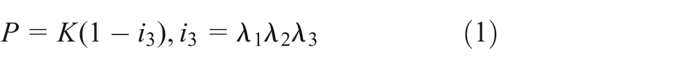
where
PR
By the classic equations of elastic materials, there is a relation between K and

where
In this article, PR was used to describe the volumetric term of rubber’s strain energy functions, whose parameters were derived from uniaxial compression and tension tests. Based on the strain energy functions, the vertical stiffness of the rubber isolator was simulated by the commercial FE software ABAQUS. The FE model was modified by adjusting the value of PR. When PR is 0.499, the simulation result is in good agreement with test data. By the modified FE model, the structure of rubber isolator was improved to meet the design request.
Constitutive models with compressibility
Rubbers are assumed isotropic, hyperelastic, and almost incompressible. Their large deformation behaviors are determined by the constitutive models described by the strain energy function W. And it is a function that means the stored strain energy on unit initial volume fraction.
22
The strain energy function W has many different forms and is usually made up with the invariants
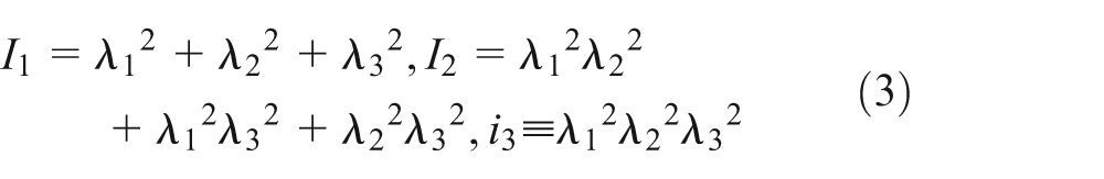
Because of the compressibility of hyperelastic materials, such as rubbers, the strain energy function W is split into two parts

where the first part
For typical hyperelastic material models, polynomial models are often used, where the strain energy function has the form


With reference to equations (2) and (7), the coefficient

So the strain energy function is
Mooney–Rivlin model
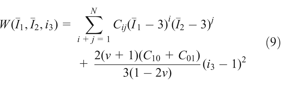
Mooney–Rivlin model 25 is the polynomial model of order N = 1. From equations (6) and (9), its strain energy function is

Mooney–Rivlin model is most commonly used. But it cannot predict the large deformation behavior of rubbers and is often used in small deformation state.
Neo-Hookean model
Neo-Hookean model
26
is a simplified form of Mooney–Rivlin model, which only has the first invariant

Yeoh model
Yeoh model 27 is proposed not to use the second invariant and it has a form more complicated than the former two models
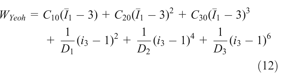
When the volume change is very small, the value of

Ogden model
Ogden model 28 is different from polynomial models, as its strain energy function is expressed in terms of principal stretches
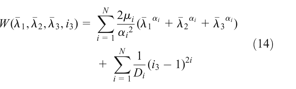
where

From equation (2),

Same as Yeoh model, the volumetric term G of W is simplified to only one part containing the coefficient D1, and the strain energy function of Ogden model is

According to Holzapfel, 30 the test data are in good agreement with the theoretical results in Ogden N = 3 model. So this model was used in this article.
Parameter identification tests
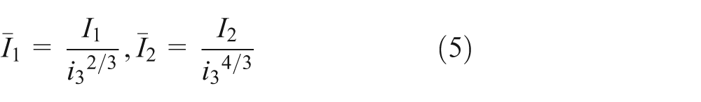
For the strain energy functions (equations (6) and (14)), the parameters
Uniaxial tension test
In Figure 1, the dumbbell specimens were cut down from a rubber sheet with thickness 2 mm, and the width of the middle area of specimens is 6 mm. According to ISO 37:2005, 31 uniaxial tension tests were performed at a universal mechanical testing machine equipped with a computerized control and measuring systems of extension and force. In Figure 2, the extensometers were used to measure the extension of the test area, and the load force was measured by load cells inside the machine. The load–displacement history was recorded and converted into stress–strain data during the tensile test. For the repeatability and consistency, three specimens were tested and the averages of test data were calculated.

Dumbbell specimens.

Uniaxial tension test.
Uniaxial compression test
In Figure 3, cylindrical specimens were used in the compression test. The dimensions of it are 29 mm diameter and 12.5 mm thickness. Same as the tension tests, three specimens were tested, and the test was in accordance with ISO 7743:2011. 32 In Figure 4, the specimen was compressed between two rigid plates. To make the specimens free to expand in the radial direction during the compression, the surfaces of top and bottom plates were coated with silicone oil to reduce the friction. Even very small levels of friction would significantly affect the measured stiffness, as Day and Miller 33 discussed in their article, the compression test must be taken carefully.

Cylindrical specimens.

Uniaxial compression tests.
Fitting constitutive models
Nominal (or engineering) stress–strain data were obtained from tension and compression tests. And the data were inputted into the FE code ABAQUS, in which the constitutive models were fitted in the least square method. 34 Four strain energy functions, Mooney–Rivlin equation (10), neo-Hookean equation (11), Yeoh equation (13), and Ogden equation (17), were chosen.
The fitted curves of different strain energy functions are shown in Figure 5. The curves of Ogden N = 3 and Yeoh strain energy functions are in good agreement with test data in all ranges of strain. Neo-Hookean and Mooney–Rivlin models can only describe rubber behavior accurately at low strain, and the fitted curves deviate from the experimental curves in large values of the stretch.

Fitted curves of different constitutive models.
To evaluate these four constitutive models, the relative error e of the stress between experimental and theoretical value was calculated

where

Relative error between experimental and theoretical results.
Through a least-squares-fit procedure minimizing the relative error in stress, the parameters
Parameter values for constitutive models.

From equation (7) and (16), bulk modulus K can be expressed in terms of PR
For neo-Hookean and Yeoh model, the form of K is the same

For Ogden model

With the values of parameters in Table 1, the relation between K and

Relation between the bulk modulus K and Poisson’s ratio
FEA
Structure of the rubber isolator
As shown in Figure 8(a), the rubber isolator consists of nine rubber pads, each of which is made up with a rubber layer bonded to two steel plates. The rubber pads were bolted together. The whole height of the rubber isolator is 1.26 m, and the diameter of the steel plate is 1.6 m. It can only bear vertical load. The rubber isolator is a part of the leg mating unit as shown in Figure 8(b), which is used in the installation of oil field platforms to reduce the dynamic load caused by the waves. The size of the rubber isolators is very large, and it is different from those commonly used in seismic bridge applications. The thickness of rubber layers is larger than bridge rubber bearings that are commonly used, as shown in Figures 12 and 18; the rubber layer could bulge in the radial direction when the rubber pad is compressed. And the lateral surfaces would touch the steel surfaces, which increases the stiffness of the rubber isolator and makes it bear more loads in extreme situation. So the diameter of the steel plates is larger than the diameter of the rubber layers.

Structure of the rubber isolators: (a) rubber isolators and (b) leg mating unit.
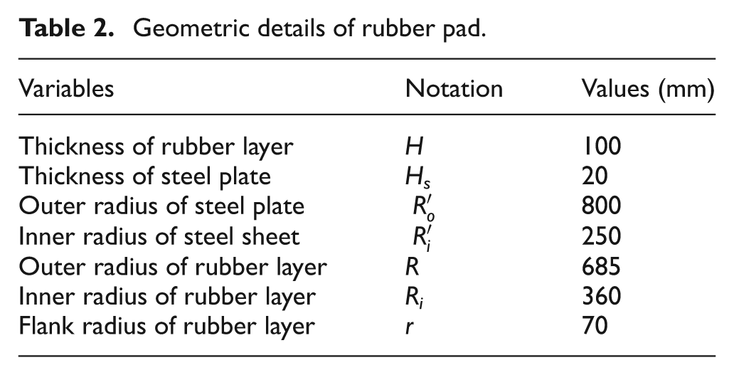
The structure of a half rubber pad is shown in Figure 9 and the geometry is defined in Table 2. The upper and lower surfaces of the rubber are bonded to rigid steel plates and are highly constrained. Only the vertical lateral surfaces of the rubber can expand freely when the rubber pad is subjected to vertical loads.
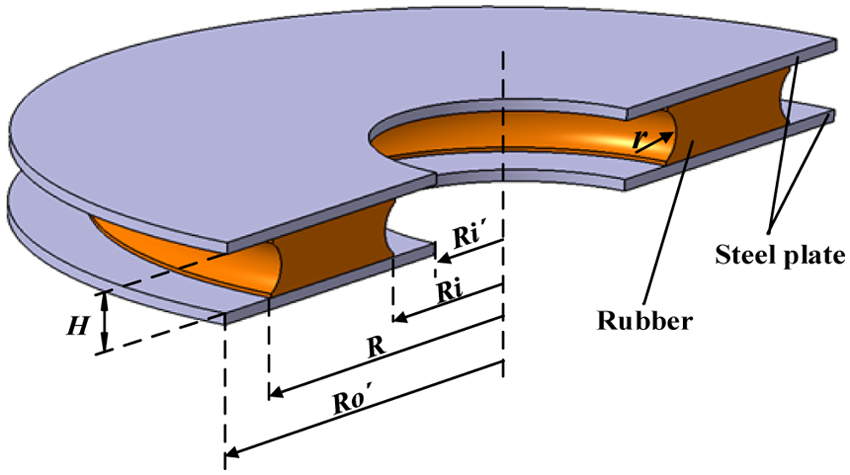
Half model of a rubber pad.
Geometric details of rubber pad.
Modeling of rubber pads
As we can see from Figure 8, the rubber pads were stacked together just like springs in series. So the characteristic of the rubber isolator can be obtained from analyzing only one rubber pad.
The two-dimensional (2D) plane FE model is shown in Figure 10. Only a half of the cross section was modeled, as the shape and load of rubber pads were axisymmetric. In numerical modeling, the axisymmetric model is used to reduce the number of elements and improve the calculation speed. The element size of the rubber pads is about 2 mm. The rubber section of the pad was modeled with plane strain four-node hybrid elements. The type of rubber and steel elements is CAX4H and CAX4R, respectively. 5
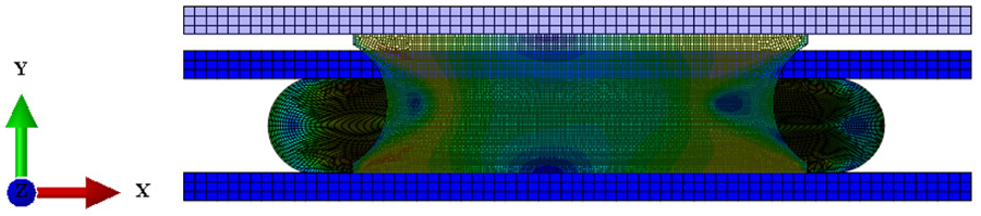
Axisymmetric FEA model: initial and deformed meshes.
The steel plates are made of low-carbon steel with material properties: PR is 0.3, and elastic modulus is 210 GPa. Rubber’s material performance is determined by strain energy functions as we discussed in section “Constitutive models with compressibility.” Four types of hyperelastic constitutive models were applied, and their parameters are defined in Table 1. To study the influence of rubber compressibility on the simulation, a range of values of PR from 0.48 to 0.49999 were defined separately, and the simulation was calculated repeatedly.
Figure 11 shows the boundary conditions and constraints of FE model. The displacement of the base steel plate was restrained in all directions. The rubber layer and steel plates were bonded together by “tie.” When the rubber pad is compressed, the rubber layer could bulge in the radial direction, and its lateral surfaces will be in contact with the surface of the steel plates. So the frictions of these contact surfaces were defined and the friction coefficient was 0.3. Displacement load was put on a reference point, which was coupled with the top steel plate. Finally, the displacement–force data of the reference point were obtained during the simulation. Although the FE model is planar, it can be displayed in three dimensions by sweeping along the Y-axis. In this way, it could be more visualized. In Figure 12, the planar elements swept 90° along the Y-axis, showing the deformation of a quarter rubber pad.
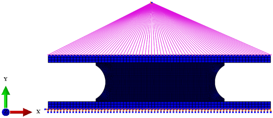
Boundary conditions and constraints of FE model.

FE model in 3D form (sweeping 90° along Y-axis).
To verify that the 2D model equals to the three-dimensional (3D) model, the two types of the FE model were simulated, and the vertical displacement was applied to the top of the pad. The displacement–force curves are shown in Figure 13. It is obvious that the two curves are almost the same, which verifies the accuracy of the 2D model.
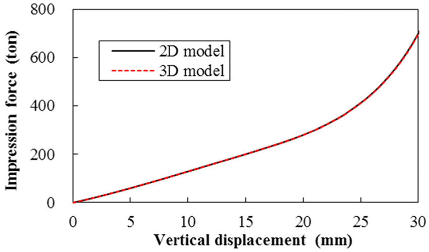
Displacement–force curves of 2D and 3D model.
Effect of bulk compressibility
To compare the simulation result to the test data of the vertical stiffness, the compression test of the rubber isolator was performed on a universal testing machine. The displacement–force history was obtained in the test. As shown in Figure 14, the universal testing machine is driven by hydraulic pressure from accumulators. And its maximum vertical load is 30 MN. In the compression test, the rubber isolator was put on the lower plate of the test machine, and the vertical force was applied to the upper plate. Vertical displacement was measured by four sensors in different locations, and the average was calculated as the measured value of the displacement. The force was measured by load cells inside the machine. And the air temperature is about 25°C.

Compression test of the rubber isolator.
Because of rubber’s nonlinear behavior of hysteresis, creep, and stress softening phenomenon, the compression speed is slow and is 6 mm/min. After six repeated load–unload cycles, the force–displacement data were measured. The compression displacement is 250 mm totally (the displacement of each rubber pad is about 28 mm).
The load–displacement history obtained from FEA is compared with the test data in Figure 15. It is clear that the value of PR has a great influence on the simulation results. The greater the value of PR, the harder it is compressed. In addition, the linear elastic material model was simulated. It is obvious that the hyperelastic model is more accurate than the linear elastic material model, especially in the large displacement.

Comparison of measured and predicted force: (a) Mooney–Rivlin, (b) Neo, (c) Yeoh, and (d) Ogden.
In all ranges of deformation, the results of Mooney–Rivlin and neo-Hookean models are similar, for the strain energy function of neo-Hookean is simplified from Mooney–Rivlin model and the parameters C10 in both models are very similar in Table 1. For these two models, the simulation stiffness of the rubber pad is nearly linear and seriously deviates from test results in large displacement, because they are one-order models and can only describe the rubber behavior accurately at low strains.24,35
When the value of PR is greater than 0.49, Ogden and Yeoh models capture the nonlinear behavior of rubber pad in large deformation successfully. For Yeoh model, the simulation results for PR = 0.499 prove a good conformity with the test data. So the hyperelastic Yeoh model is taken for further analysis, and the value of PR is set to 0.499.
In this article, the static stiffness of the rubber pad is defined as the ratio between the load and the vertical displacement of the top steel plate. When the vertical displacement is 27 mm, the static stiffness of the rubber pad with different values of PR is shown in Figure 16. The static stiffness can be greatly influenced by PR. When the value of PR is less than 0.48, the stiffnesses of four hyperelastic constitutive models are similar, and the relation between load and PR is linear. But when the value of PR is larger than 0.49, the stiffness varies in different constitutive models, and the stiffness increases rapidly as PR increases. It emphasizes the importance of compressibility in FE simulation of rubber-like materials. In addition, PR could be used to modify the FE model to improve the accuracy.
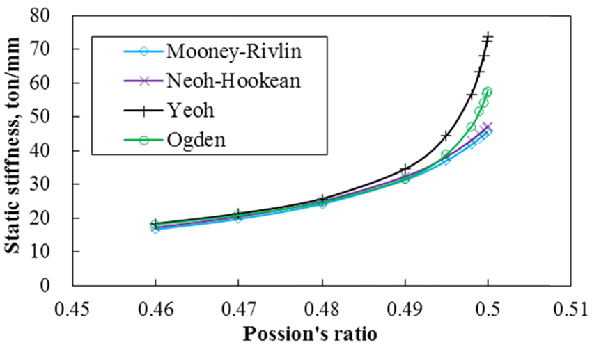
Static stiffness for various Poisson’s ratio (vertical displacement is 27 mm).
Structure improvement
Knowledge of the modified FE model by PR makes it possible to improve the rubber pad structure to meet the design request. According to the test and simulation results, the initial structure of the rubber pad should be improved for the reasons: (1) cracks could appear on the lateral surfaces of rubber pads in compression and (2) the initial static stiffness is larger than the design value.
Analysis of crack
When the rubber pad is compressed in the vertical direction, the vertical lateral surfaces of it could bulge horizontally. But in some conditions, cracks would appear on the middle of the bulged lateral surface. For instance, the crack is shown in Figure 17. During the compression test, the probability of crack occurrence varies with the value of the flank radius r (Figure 9), and the cracks appear on the rubber pad with the large r more often than those with the small r. So it is important to analyze the influence of the flank radius r on the distribution of the stress field.

Cracks on the rubber pad.
The stress field of the rubber pad’s cross section is shown in Figure 18. The red color means a large value of stress while blue means a small value. The lateral surface is all in red especially in the middle of it. The stress along the rubber’s lateral surface in the Y-direction is shown in Figure 19. It is clear that the stress is high in the middle of the lateral surface, which is in agreement with the location of the crack in Figure 17. The stress decreases as the value of r decreases. The stress is sensitive to r when its value is less than 70 mm. While the value of r is larger than 80 mm, the change in the stress is neglectable as r increases. So the value of r has been changed to 50 mm to reduce the stress and avoid the cracks. In Figure 20, the stiffness of rubber pads can hardly be influenced by the values of r.
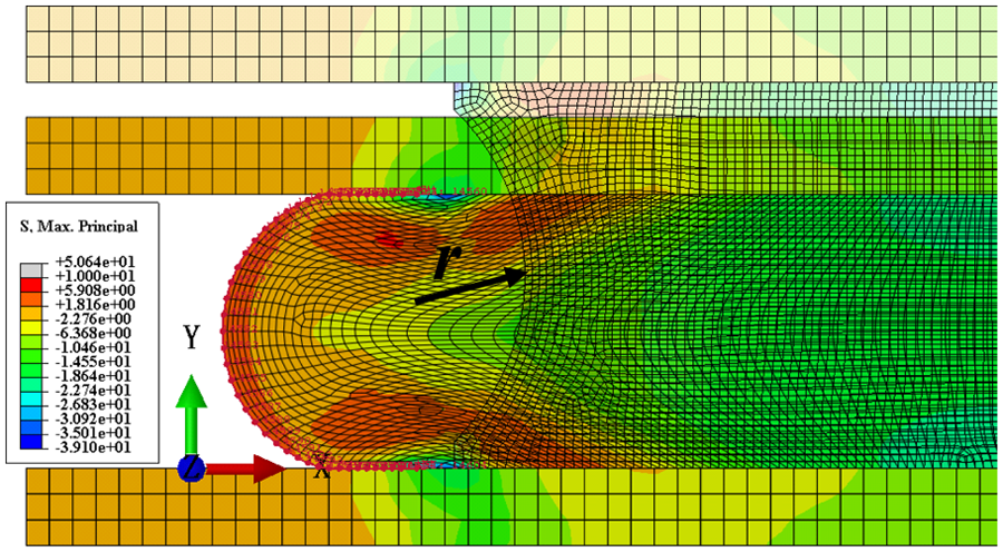
Stress field in the rubber pad (initial and deformed meshes, r = 70 mm, vertical displacement is 29 mm).
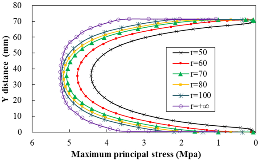
Stress on the vertical lateral surface in Y-direction.
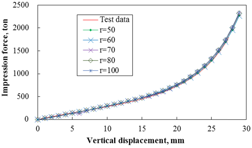
The stiffness of rubber pads with different values of r.
Adjustment of stiffness
As shown in Figure 21, the design stiffness of the rubber pad is 1100 ton as the vertical displacement is 25 mm, which means the static stiffness is 44 ton/mm and equals to 440 kN/mm. The maximum design displacement of the rubber pad in the vertical direction is 32 mm, while the thickness of the rubber pad is 100 mm. Due to limitations of the structure and process, only the parameter outer radius R (Figure 9) could be changed to meet the desired stiffness. By FEA, the stiffness of rubber pads with different radius is shown in Figure 21. As the outer radius increases, the vertical stiffness also increases. In the vertical direction, the force and displacement behavior is linear in the small range of load. But when the vertical displacement is beyond 20 mm, the nonlinearity of the stiffness is obvious. When the value of the outer radius is 670 mm, the stiffness approaches 1100 ton. So the outer radius of the rubber pad is changed to 670 mm.

Displacement–force curves of rubber pads with various R.
Experimental verification
By FEA, the values of R and r have been changed to 670 and 50 mm. As described in section “Effect of bulk compressibility,” the compression test of the improved structure was performed to get the displacement–force history. The improved rubber isolator under compression is shown in Figure 22. There is no crack appearing on the vertical lateral surfaces during the test. In Figure 23, the vertical stiffness of the rubber pad under pure compression obtained by FEA is in good agreement with the test data. The maximum deviation between the test data and the simulation is only 5.1% at the vertical displacement 29 mm. It proves the accuracy of the FE model modified by PR, and it could be used to provide guidance for the design and production of rubber isolator.

The improved structure under compression.

Displacement–force curves of the improved structure.
Conclusion
The conclusion is as follows:
For the structure of a rubber pad bonded to rigid plates, the static stiffness is very sensitive to bulk compressibility.
Stress on the lateral surfaces could be decreased by adjusting the flank radius without changing the stiffness of rubber pad of rubber isolators.
PR could be used to modify the FE model to improve the simulation accuracy. And it could provide guidance for the design and production of rubber isolator.
Yeoh and Ogden constitutive models are more accurate than Mooney–Rivlin and neo-Hookean models in the FE simulation of rubber isolators. Yeoh and Ogden constitutive models fit the stress–strain data of rubber specimens more accurately than the other two models. Compared with the test results, the stiffness of rubber pads simulated with the former two models is more accurate than with the latter two models.
Footnotes
Academic Editor: Filippo Berto
Declaration of conflicting interests
The author(s) declared no potential conflicts of interest with respect to the research, authorship, and/or publication of this article.
Funding
The author(s) received no financial support for the research, authorship, and/or publication of this article.