Sage Journals: Discover world-class research

Abstract

This article introduces the β phase plane method to determine the stability state of the vehicle and then proposes the electronic stability program fuzzy controller to improve the stability of vehicle driving on a low adhesion surface at high speed. According to fuzzy logic rules, errors between the actual and ideal values of the yaw rate and sideslip angle can help one achieve a desired yaw moment and rear wheel steer angle. Using genetic algorithm, optimize the fuzzy controller parameters of the membership function, scale factor, and quantization factor. The simulation results demonstrate that not only the response fluctuation range of the yaw rate and sideslip angle, but also the time taken to reach steady state are smaller than before, while reducing the vehicle oversteer trend and more closer to neutral steering. The optimized fuzzy controller performance has been improved.

Keywords

Sideslip angle yaw rate β phase plane method fuzzy electronic stability program genetic algorithm

Introduction

The main reason for traffic accidents is that the vehicle loses stability when driving at high speed. In recent decades, to enhance vehicle stability driving on low adhesion roads, vehicles were equipped with four-wheel steering (4WS), traction control system (TCS), and electronic stability program (ESP). Although the 4WS can reduce sideslip angle to nearly zero when the vehicle turns, it becomes less effective when tire’s lateral force approaches the limit of adhesion, and vehicle dynamics show nonlinear characteristics.¹

The TCS system was designed to maximize the contact forces between the tires and the road during braking and acceleration.² TCS controls the output torque of the driving wheels to control the tires’ longitudinal force. This is not available in the braking condition. Therefore, the application scope of TCS is limited.

The tire friction circle principle demonstrates that the lateral force margin is less than the margin of the wheel longitudinal force and lateral force, and therefore, the longitudinal force does not necessarily reach saturation.

However, as the vehicle goes into the limit-handling region and nonlinearity becomes significant at a high lateral acceleration range, it becomes unstable, unfamiliar to the drivers, and eventually difficult to maneuver.³ The active rear wheel steering (ARS) system employs the rear wheel steering angle as the only control input and selects either sideslip angle or yaw rate as the control target.⁴

To ensure the stability of the vehicles in the nonlinear area, one can apply an ESP intervention, which is the use of unsaturated tire longitudinal force on the vehicle yaw and lateral movement, thereby improving the vehicle’s turning stability in extreme conditions. ESP generates yaw moment, and direct yaw moment control is the advanced control system used to improve the dynamic performance of road vehicles under various road conditions.^5–7 ESP is introduced to control the yaw motion and prevent oversteering and understeering.² Direct yaw moment has a higher ability to stabilize the vehicle motion than active steering control.⁸

This article introduces the rear wheel steer angle to maintain sideslip angle in an ideal range and then combines the additional yaw moment and rear wheel steer angle to improve the lateral movement stability. Introduce the β phase method to judge the stability state of the vehicle. The designed ESP fuzzy controller depends on the result of $\overset{\cdot}{β} - β$ phase plane method to control the vehicle’s stability or not. To overcome the limitation of the design flaw of fuzzy controller, using genetic algorithm optimize the parameters and membership function. Simulation test of low adhesion road was used to verify the proposed controller performance.

Vehicle dynamic model

Modeling analysis is an important means of control theory research. This article required the building of the following models: the 8-degree-of-freedom nonlinear vehicle dynamic model, the 2-degree-of-freedom vehicle model, and the Gim tire model.

Eight-degree-of-freedom vehicle dynamic model

The 8-degree-of-freedom dynamic model is utilized for simulation research. This model includes a longitudinal, lateral, and horizontal pendulum and four-wheel rotation. The corresponding mechanical analysis of the vehicle is shown in Figure 1:

Longitudinal movement

m (\overset{•}{v_{x}} - v_{y} \cdot w_{r}) = (F_{x 1} + F_{x 2}) \cos δ - (F_{y 1} + F_{y 2}) \sin δ + F_{x 3} + F_{x 4}

(1)

Lateral movement

m (\overset{•}{v_{y}} + v_{x} \cdot w_{r}) = (F_{y 1} + F_{y 2}) \cos δ + (F_{x 1} + F_{x 2}) \sin δ + F_{y 3} + F_{y 4}

(2)

Yawing motion

I_{z} \cdot \overset{•}{w_{r}} = a (F_{y 1} + F_{y 2}) \cos δ + \frac{T_{f}}{2} (F_{y 1} - F_{y 2}) \sin δ + \frac{T_{f}}{2} (F_{x 2} - F_{x 1}) \cos δ + \frac{T_{r}}{2} (F_{x 4} - F_{x 3}) - b (F_{y 3} + F_{y 4})

(3)

Roll motion

I_{x s} \cdot \overset{•}{P} - m_{s} \cdot h_{s} \cdot ({\overset{•}{v}}_{x} + w_{r}) = m_{s} \cdot g \cdot h_{s} \sin φ - (k_{ϕ f} + k_{ϕ r}) φ - (C_{ϕ f} + C_{ϕ r}) p

(4)

Wheel rotational balance equation

\begin{array}{l} I_{w} \cdot w_{i j}^{•} = - R_{w} \cdot F_{x i j} + T_{d i j} - T_{b i j} \\ i j = f l, f r, r l, r r \end{array}

(5)

Figure 1.

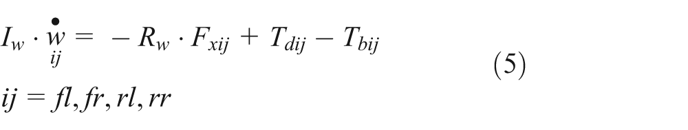
Eight-degree-of-freedom vehicle dynamic model diagram.

Gim tire model

The Gim tire model^9,10 has the characteristics of quick calculating speed, adaptability, and high precision, especially in case of the large tire slip angle. Its accuracy is far better than that for other tire models. In this section, we selected the Gim tire model to calculate the longitudinal and lateral forces of the tire.

Desired vehicle model

The linear 2-degree-of-freedom model reflects drivers’ expected vehicle steering characteristics. Yaw rate is a crucial signal for the motion control systems of ground vehicles.

The 2 degrees of freedom in a linear model allows for calculating the vehicle’s yaw rate and sideslip angle expectations as follows:

Steady-state yaw rate

w_{r} = \frac{u / L}{1 + K \cdot u^{2}} \cdot δ

(6)

where $K = (m / L^{2}) \cdot ((a / k_{2}) - (b / k_{1}))$ is the stability coefficient.

As the vehicle’s lateral acceleration value cannot exceed a maximum acceleration determined by the adhesion coefficient µ of the tire and the road surface condition, we have the following formula

w_{r \max} \leq \frac{μ \cdot g}{u}

(7)

The nominal value of the yaw rate can be expressed as follows

w_{rd} = \min {| w_{r} |, | w_{r \max} |} \cdot sgn (δ)

(8)

Generally, the reference sideslip angle is given as zero to ensure stability,¹¹ whereas the reference yaw rate is defined in terms of vehicle parameters, longitudinal speed, and the driver’s steering input.¹²

A steady-state desired slip angle (see equation (9)) is deduced based on a 2-degree-of-freedom vehicle model in Rajamani.¹² However, a zero slip angle is selected for the desired response in Nagai et al.¹³ and Boada et al.¹⁴ Using 2 degrees of freedom and the simultaneous equations, we can obtain the vehicle’s sideslip angle

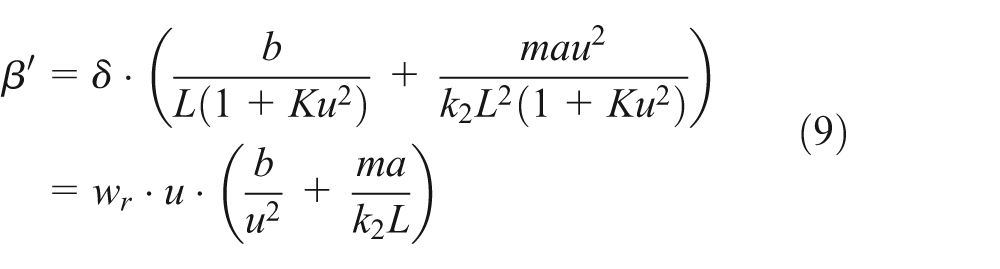
\begin{matrix} β' & = δ \cdot (\frac{b}{L (1 + K u^{2})} + \frac{ma u^{2}}{k_{2} L^{2} (1 + K u^{2})}) \\ = w_{r} \cdot u \cdot (\frac{b}{u^{2}} + \frac{ma}{k_{2} L}) \end{matrix}

(9)

Taking into account the ground conditions attached to confront limits, the sideslip angle can be expressed as follows

β'_{\max} = μ g (\frac{b}{u^{2}} + \frac{ma}{k_{2} L})

(10)

In considering the nominal sideslip angle, the vehicle should reach the value of the sideslip angle taking into account the physical limits at the same time. If the vehicle sideslip angle reaches the feature value, the vehicle will become uncontrollable and enter dangerous conditions.

The desired slip angle response cannot always be obtained when the tire force exceeds the tire’s adhesion limit. Thus, the desired slip angle has an upper bound, which can be expressed as follows¹²

β_{T} = ta n^{- 1} (0.02 μ g)

(11)

From the above formula, we can obtain the adhesion coefficient under the center of mass of sideslip angle limit value, as shown in Table 1.

Table 1.

Sideslip angle of the center of mass of the adhesion coefficient under the limit.

Parameter	Value
µ	0.2	0.4	0.5	0.6	0.8	1
β_T	2.24	4.48	5.6	6.71	8.91	11.1

Table 1 shows that the limit of the sideslip angle decreases with an increasing road adhesion friction coefficient. Especially on a low adhesion road, the centroid sideslip angle itself is very small and is more difficult to control precisely, so this article introduced the β phase plane law.

Therefore, the nominal value of the sideslip angle is given by

β_{d} = \min {| β' |, | {β'}_{\max} |, | β_{T} |}

(12)

ESP control strategy

ESP can generate the stabilizing yaw moment based on the steering angle, vehicle sideslip angle, wheel speed, yaw rate, and lateral acceleration.¹⁵ To improve the vehicle handling stability, the yaw rate (the yaw velocity of the chassis) and the sideslip angle (the angle between the directions of the velocity and chassis) of the vehicle should be controlled to follow their target values.¹⁶

Select the control variables

Yaw rate and sideslip angle are important variables describing vehicle stability. In the vehicle stability control process, sideslip angle β and yaw rate ω_γ are the two states of the vehicle’s lateral dynamics.¹⁷

Introduction of $β - \overset{\cdot}{β}$ phase plane method

First of all, to avoid ESP, control the vehicle frequently. Second, in the low friction road, the limitation of the sideslip angle is very small, and it is difficult to control it to follow the desired value. Sideslip angle β and its change rate were used to judge the vehicle’s stability, namely, using the $β - \overset{\cdot}{β}$ phase plane method.¹⁸ This method is used to study the relationship between the phase plane method sideslip angle and vehicle stability. Regarding the phase plane method’s determining the stability condition of the vehicle, Yamamoto and colleagues^19,20 and He²¹ offered a detailed in-depth discussion. The following briefly discusses the basic theory.

Figure 2 describes the phase trajectory of the stable and unstable vehicle. Obviously, in Figure 2, the portion enclosed by the two boundary lines represents the stable area of the vehicle; therefore, according to the boundary line equation, the vehicle stability criterion can be derived as follows

| B_{1} \overset{\cdot}{β} + B_{2} β | \leq 1

(13)

Figure 2.

Phase trajectory of centroid sideslip angle and its change rate.

When the above inequality holds, the vehicle driving state is stable. Once the inequality relationship is broken, the vehicle will lose its stability. The coefficients B₁ and B₂ are constants. The documents of Yamamoto and colleagues^19,20 and He²¹ discussed these in detail. The vehicle’s related parameters determine the values to be B₁ = 2.41 and B₂ = 9.615.

Vehicle stability determination condition

To avoid the ESP system intervene so frequently that influence passengers' comfort and cause drivers psychological pressure. We use the following equation (14) to determine the yaw rate of the tolerance band

| Δ r | = | w_{r} - w_{rd} | < | C \cdot w_{r} |

(14)

where C is a constant. Based on the literature review, this article considered C = 0.165. We combined the inequalities (13) and (14).

These two inequalities form the basis for determining vehicle stability. As long as one of them is not satisfied, the vehicle loses its stability. Then, ESP would intervene and control the vehicle.

The method of controlling vehicle stability

It is difficult to control the sideslip angle and yaw rate directly. It is necessary to choose an intermediate variable to control these two variables’ parameters that should be easy to control the two variables simultaneously. In this article, we choose the yaw moment as an intermediate variable. ΔM is the external yaw moment generated by the longitudinal forces of the left- and right-side wheels.¹⁷

However, increasing the braking force can be achieved at any conditions. Therefore, control the wheels braking force as a vehicle stability control method.

After calculating the yaw moment, which recovers the stability of the vehicle through allocating different braking forces to the wheels to control the vehicle’s yaw motion, the vehicle will return to the steady state quickly. The ESP control strategy schematic diagram is shown in Figure 3.

Figure 3.

Flowchart of ESP control strategy.

Additional yaw moment allocation strategy

From the characteristics of the tire to known that the tire longitudinal force margin is usually greater than the tire lateral force. Under such conditions, controlling longitudinal tire forces is an effective method to maintain the stability of the vehicle’s lateral motion.²² The transverse distribution of the vehicle’s braking force between the wheels is the most common approach to generate the required yaw moment.²³

In summary, this article uses a unilateral wheel braking strategy: braking on one side wheels includes the front and rear wheels at the same time. ΔM is the vehicle steady recovery required for additional yaw moment. If you brake the left-side wheels, you obtain

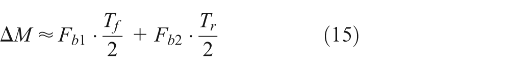
Δ M \approx F_{b 1} \cdot \frac{T_{f}}{2} + F_{b 2} \cdot \frac{T_{r}}{2}

(15)

where F_b₁ and F_b₂ denote the left front and rear wheel braking forces, respectively, and T_f and T_r denote the wheel front and rear tracks, respectively. Since the vehicle’s front and rear tracks are almost equal, we have

F_{b 1} + F_{b 2} \approx \frac{Δ M}{(T_{f} + T_{r}) / 4}

(16)

Based on this principle of distribution applied to the left-side front and rear wheels, brake torque can be expressed as follows

T_{b 1} = \frac{F_{Z 1}}{F_{z 1} + F_{z 2}} \cdot \frac{Δ M}{(T_{f} + T_{r}) / 4} \cdot r

(17)

T_{b 2} = \frac{F_{Z 2}}{F_{z 1} + F_{z 2}} \cdot \frac{Δ M}{(T_{f} + T_{r}) 4} \cdot r

(18)

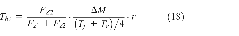
The ESP is required to control the braking torque of right-side wheels. By the same token, it can be calculated.

Determine of vehicle steering characteristic

Based on the ESP braking force allocation strategy, under different circumstances, according to the vehicle front wheel’s steering angle and the difference between the actual and nominal yaw rates, we can find out the direction of the compensation torque and braking wheels of the vehicle. We established Table 2 according to this law.

Table 2.

Principle of how to select braking wheels.

Nominal yaw rate W_ro	Deviation of yaw rate (W_r − W_ro)		Steering characteristics	Brake wheel	Remark
W_ro > 0 (turn left)	≥0	W_r > 0, W_ro > 0; W_r > W_ro	Oversteer	Right-side front and rear wheels	Define turning left as the positive direction, setting counterclockwise yaw moment, and δ is positive
	<0	W_r > 0, W_ro > 0; W_r < W_ro	Understeer	Left-side front and rear wheels
		W_r < 0, W_ro > 0
W_ro < 0 (turn right)	>0	W_r < 0, W_ro < 0; W_r > W_ro	Understeer	Right-side front and rear wheels
		W_r > 0, W_ro < 0
	≤0	W_r < 0, W_ro < 0; W_r < W_ro	Oversteer	Left-side front and rear wheels

Establish fuzzy controller for ESP system

Fuzzy logical control is not only a typical nonlinear control method but also has good adaptability and robustness character.

ESP control strategy

According to two input variables, the controller can output yaw moment and rear steer angle through manually setting appropriate rules and then assigning wheel braking force to control vehicle stability under extreme conditions.

Based on the experience of designing the fuzzy controller directly, experts do not rely on the controlled object model. Instead, they control the complex, nonlinear, large delay and uncertainty.²⁴ It is the biggest advantage comparing classical and modern control theory. Therefore, in this article, we selected fuzzy control strategy for the ESP system.

Design of fuzzy controller

As previously analyzed, the purpose is that the vehicle sideslip angle and yaw rate follow the expected ideal vehicle model. Therefore, the main objective of the ESP fuzzy controller is to minimize deviation of the actual response to the expected value. Obviously, these two deviations should be used as two inputs of the fuzzy controller

\begin{matrix} Inputs : e (β) = β - β_{d}; e (W_{r}) = W_{r} - W_{rd} \\ Outputs : Δ M; δ r \end{matrix}

Obviously, the designed fuzzy controller is a dual input and dual output controller. The language input and output variables of the fuzzy subsets are divided into seven parts, namely each have seven language value:

\begin{matrix} {e (β), e (W_{r})} = {NB, NM, NS, ZE, PS, PM, PB} \\ {Δ M, δ r} = {NB, NM, NS, ZE, PS, PM, PB} \end{matrix}

Depending on the input and output variables of the basic scope of the domain size, to facilitate processing, the domain is transformed into the fuzzy domain [−6, 6]. According to the actual situation of the input and output variables, we set Ke(β) = 60, Ke(w_r) = 30, K_ΔM = 1000, and K_δr = 0.015. The diagram of the fuzzy controller is shown in Figure 4.

Figure 4.

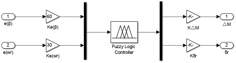
Diagram of the fuzzy controller.

Define fuzzy variable subset

The sharper the membership function, the higher the resolution. With the corresponding fuzzy control variables, control is more sensitive. The membership function of these variables is shown in Figures 5 –8. Due to the triangular membership function has the high sensitivity characteristic, for the ESP nonlinear system,select triangular membership functions to improve the response speed of the system.

Figure 5.

Membership function of e(W_r).

Figure 6.

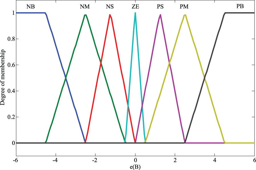
Membership function of e(β).

Figure 7.

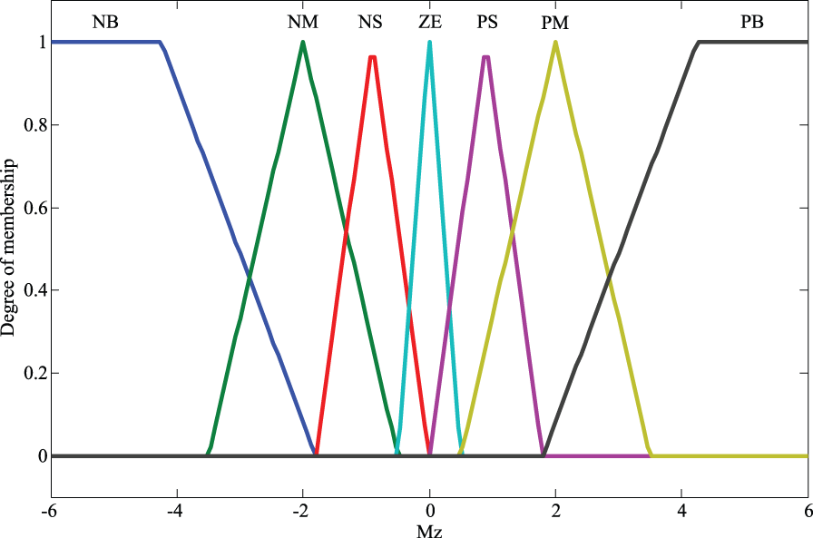
Membership function of ΔM.

Figure 8.

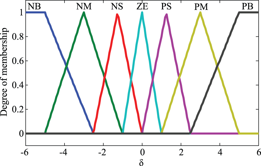
Membership function of δr.

The outputs of fuzzy logic rules of additional yaw moment ΔM and δr are described in Table 3.

Table 3.

ESP fuzzy logical rules.

e(β)	NB		NM		NS		ZE		PS		PM		PB
e(W_r)	ΔM	δr	ΔM	δr	ΔM	δr	ΔM	δr	ΔM	δr	ΔM	δr	ΔM	δr
NB	PB	PB	PB	PM	PB	PS	PM	ZE	PB	NS	PB	NM	PB	NB
NM	PB	PB	PB	PM	PB	PS	PM	ZE	PB	NS	PB	NM	PB	NB
NS	PS	PM	PS	PB	NS	PM	PS	ZE	PM	ZE	PM	NS	PB	NS
ZE	ZE	PB	ZE	PB	NS	PM	ZE	ZE	PS	NM	ZE	NB	ZE	NB
PS	NB	PS	NM	PS	NM	ZE	NS	ZE	PS	NM	NS	NB	NS	NM
PM	NB	PB	NB	PM	NB	PS	NM	ZE	NB	NS	NB	NM	NB	NB
PB	NB	PB	NB	PM	NB	PS	NM	ZE	NB	NS	NB	NM	NB	NB

Simulation test

To study the performance of the proposed controller, simulations were conducted in Simulink based on an 8-degree-of-freedom vehicle model.

Sine condition

In the process of the simulation, the vehicle runs at a speed of 100 km/h and then at time t = 2 s, the steering wheel angle experiences a sine change with an amplitude of 0.262 rad and a frequency of 0.25 Hz, as shown in Figure 9(a) (δf = 0.262 rad, f = π/2). The road adhesion coefficient is µ = 0.2. This condition simulates the vehicle driving at high speed and changes the double lane to avoid an obstacle.

Figure 9.

(a) Front wheel angle, (b) $β - \overset{\cdot}{β}$ phase trajectory of the vehicle with ESP and no control and contrast of $β - \overset{\cdot}{β}$ phase stability area and actual $β - \overset{\cdot}{β}$ phase trajectory, (c) contrast of the error of yaw rate, (d) contrast of the error of sideslip angle, (e) braking torque, (f) additional yaw moment, and (g) additional rear wheel steer angle.

Depending on the $β - \overset{\cdot}{β}$ phase trajectories in Figure 9(b) and (c), the phase trajectories of the vehicle without ESP suggest that the driver has lost control of the vehicle. Nevertheless, the phase of the vehicle equipped with ESP can converge to a bit, which indicates a vehicle in a stable state. According to Figure 9(d), the yaw rate of the vehicle without ESP achieves −0.5 rad/s, far exceeding the ideal value, the vehicle slips severely. The vehicle equipped with ESP can track the ideal yaw rate well. As Figure 9(e) shows, in the vehicle without ESP, the maximum value of sideslip angle has exceeded 0.039 rad, so the actual driving path gravely deviates from the driver’s expectations. With ESP, the sideslip angle of the vehicle will fluctuate within a narrow range due to vehicle steering, but it also can be a good track over sideslip angle, showing excellent transient characteristics.

Ramp step condition

During the simulation process, the vehicle speed is 100 km/h for 1 s, and the steering wheel angle goes through a step change in the amount of 0.14 rad, as shown in Figure 10(a). The road adhesion coefficient is µ = 0.2. The position of the accelerator pedal remains unchanged during the maneuver. This condition is similar to a vehicle driving at high speed, with sudden large steering angles in the front wheel.

Figure 10.

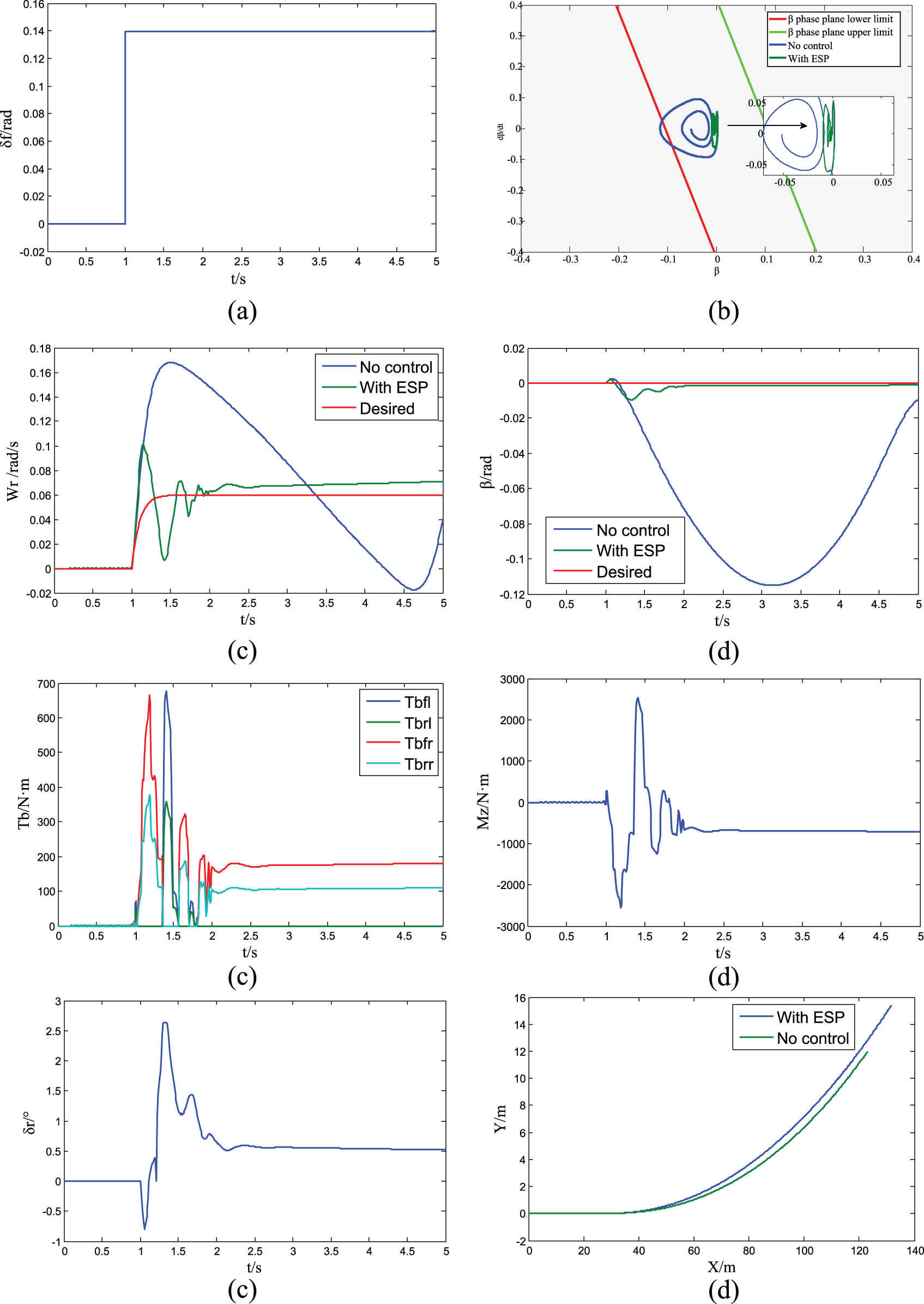
(a) Equivalent front wheel angle, (b) $β - \overset{\cdot}{β}$ phase trajectory of the vehicle with ESP and no control, and contrast of $β - \overset{\cdot}{β}$ phase stability area and actual $β - \overset{\cdot}{β}$ phase trajectory, (c) the yaw rate error in a low adhesion ramp step condition, (d) error in sideslip angle in a low adhesion ramp step condition, (e) braking torque, (f) additional yaw moment, (g) additional rear steer angle, and (h) vehicle trajectory.

Simulation results

In the vehicle with ESP, the yaw rate can approach the ideal value in a short time, about 1 s, to a steady-state value of about 0.007 rad, as shown in Figure 10(e). This is only a matter of keeping a small steady-state error with ideal yaw rate, as shown in Figure 10(e). And the shock is extremely small; at time t = 2 s, the vehicle can turn smoothly. The vehicle achieved the desired steering characteristics with ESP control. The sideslip angle of the vehicle without ESP generated relatively large fluctuations, up to a maximum value of about 0.11 rad in Figure10(f). During the simulation process, fluctuations always exist; at the end of the simulation, it still has not reached a plateau, indicating the presence of the body swing phenomenon that running on a low friction coefficient road is very dangerous.

The phase of $β - \overset{\cdot}{β}$ in Figure 10(b)–(d) can be seen. Although phase trajectory tends to converge no matter whether the vehicle has ESP, the phase track scope of the vehicle with ESP is smaller than the vehicle without. Therefore, without ESP control, the vehicle’s center of mass, sideslip angle, and yaw rate change drastically. Under outside interference, the vehicle usually loses control and stability.

It takes a long time to determine the membership function, control rules, scaling factor, and quantization factor of the fuzzy controller. The design process mainly relies on the trial-and-error experience of the operator or designer. Furthermore, it is impossible to acquire the optimized system.

In recent years, some researchers have tried to apply genetic algorithms to optimize the fuzzy controller; using a genetic algorithm could reduce the effect of the designers’ subjective experience. In this article, we take a genetic algorithm to optimize the distribution of membership functions and determine the optimal scaling factor and quantization factor of the controller.

In Figure 10, al, a2, and a3 are the membership functions for the two adjacent intersections’ ordinate (called the overlap factor). The overlap factor reflects the completeness characteristic of the membership function. In this article, the symmetry characteristic of the membership function distribution only needs to determine four optimal widths “l_HG, l_FE, l_DC, l_BA” and three overlapping factors with an optimal value of a1, a2, and a3 (0 < a < 1), which are shown in Figure 11.

Figure 11.

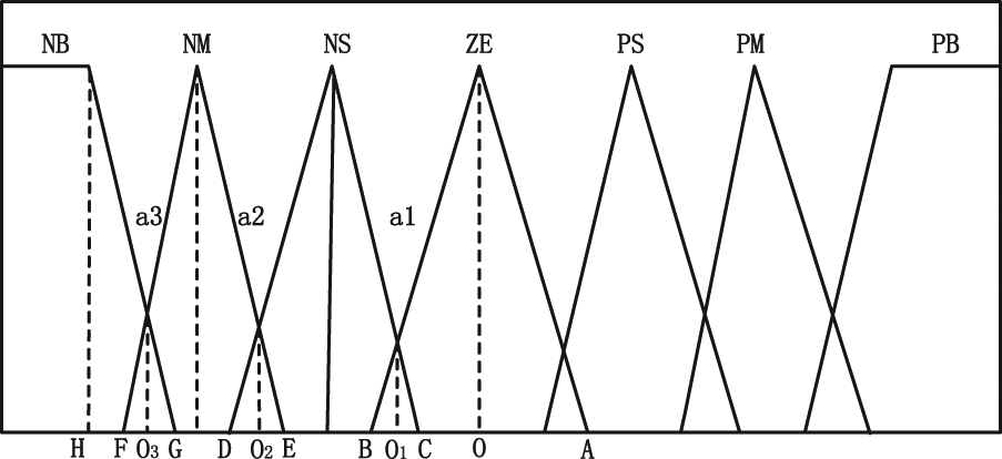
Membership function optimization.

Obviously, when the seven parameters were determined, the horizontal ordinate values A–H and the membership functions’ centers O₁, O₂, and O₃ can be calculated using the geometric diagram. According to the symmetry, the optimal distribution curve membership function of the entire region can be determined (Figure 12).

Figure 12.

Real number coding sequence of the membership functions.

To ensure completeness of the membership functions and a reasonable width, in this article, we set the value range of the overlapping factors a1, a2, and a3 as [0.2, 0.8], the width of the L_HG as [0.5, 4], and the value of I_FE, I_DC, and I_BA as [0.5, 3]. For the structure of a string variable membership function, it is necessary to use seven real numbers. The ESP and the entire fuzzy controller should include two input variables and two output variables, but each chromosome should comprise 7×4 = 28-bit real number components.

The fuzzy controller is directly connected to the controlled object and does not establish a precise mathematical model for the actual object, resulting in more difficulty to select the fitness function. Studies have shown in Boada et al.¹⁴ that the time-domain performance integral time absolute error (ITAE) control system has a smaller rapid and smooth dynamic performance, a smaller overshoot, a shorter rise time, and a faster transition process, which is the preferred performance evaluation function for a design control system. The specific expression is

J_{ITAE} (t) = \int_{0}^{T} t | e (t) | dt

(19)

In this article, to improve the sideslip angle and yaw rate of transient characteristics comprehensively, after adding both their own ITAE performance value and taking the reciprocal as the fitness function, we have the following

f (i) = \frac{1}{(J_{β ITAE} + J_{rITAE})}

(20)

The Roulette selection operation has a consistent crossover and mutation operation using the basic alleles. The process using genetic algorithms to optimize the distribution of the membership functions is shown in Figure 13.

Figure 13.

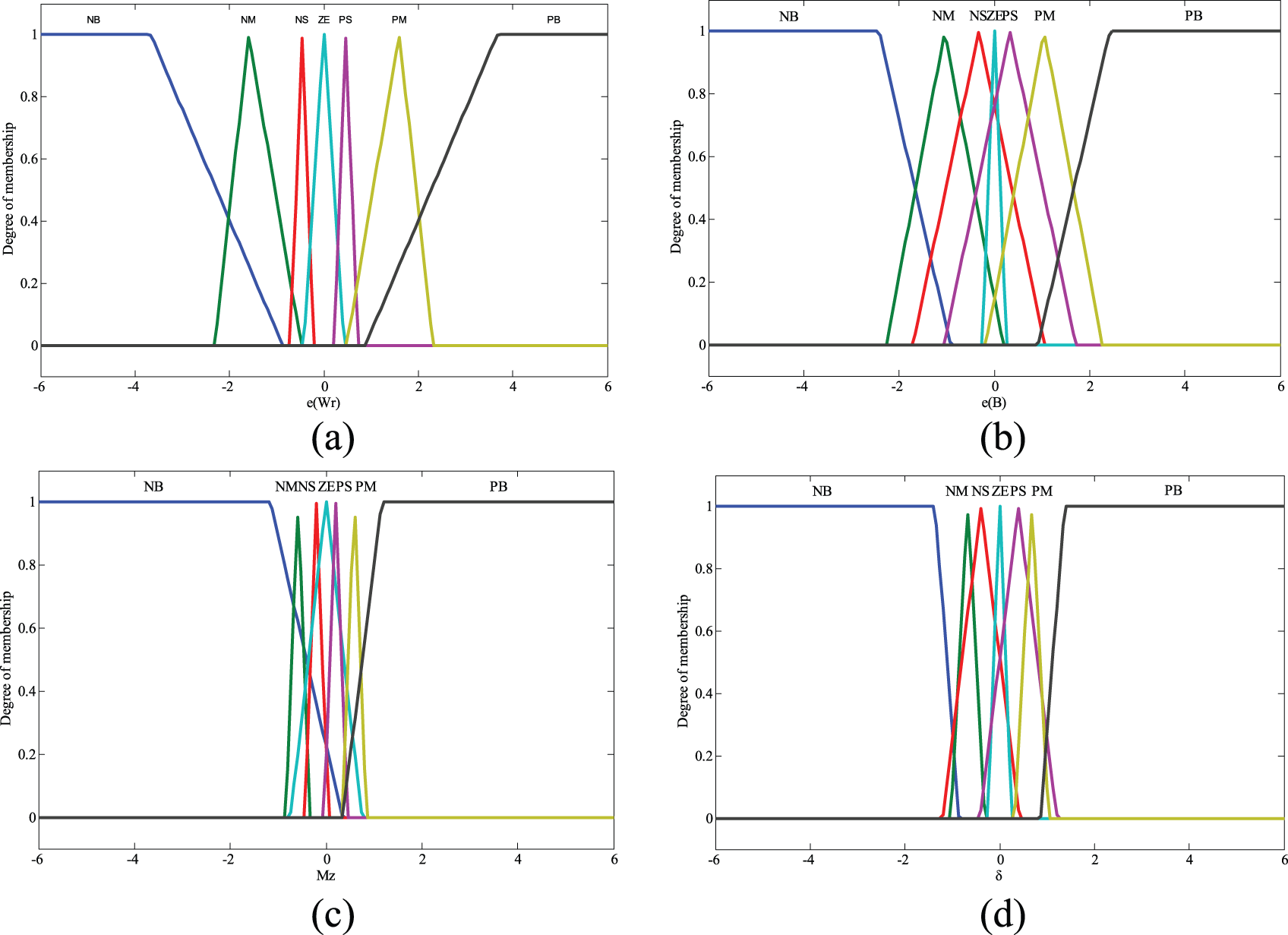
(a) Optimized membership function of e(W_r), (b) optimized membership function of e(β), (c) optimized membership function of ΔM, and (d) optimized membership function of δr.

In this article, we set 30 generations and selected the size of the population to be 50, with a crossover probability of 0.9 and mutation probability of 0.01. The simulation test on a low adhesion coefficient road took continuous sinusoidal input until it reached the set maximum hereditary algebra. Using the same methods, we performed 4-bit real coding for the scale factor of the fuzzy controller input variables Kβ and Kw_r and the quantization factor of output variables KΔM and Kδr.

With the above optimization distribution curve, membership functions, and fuzzy rules as known, then we used genetic algorithms to optimize these four parameters. Ultimately, the optimum values of these four parameters are shown in Table 4. The comparison of simulation results before and after optimization is shown in Figure 14.

Table 4.

The GA optimization results of scale factor and quantization factor.

Parameters	Scale factor/quantization factor	After GA—ESP parameters
Ke(β)	60	71
Ke(w_r)	30	51.5
KΔM	1000	1276
Kδr	0.015	0.0165

GA: genetic algorithm; ESP: electronic stability program.

Figure 14.

(a) Contrast of yaw rate response between ESP and GA-ESP in the sine condition, (b) contrast of sideslip angle response between ESP and GA-ESP in the sine condition, (c) contrast of yaw rate response between ESP and GA-ESP in the ramp condition, (d) contrast of sideslip angle response between ESP and GA-ESP in the ramp condition, (e) contrast of sideslip angle response, and (f) contrast of sideslip angle response with ESP and GA-ESP in the ramp condition.

Conclusion

In this article, we used an ESP fuzzy control system based on direct yaw moment and rear steering angle control to maintain the stability of the vehicle within a range of its $β - \overset{\cdot}{β}$ phase. We presented it under normal conditions. The yaw moment to control vehicle stability was assigned to the left- or right-side wheels of the vehicle by applying brake force and an additional rear wheel steering angle to decrease the sideslip angle. With the 8-degree-of-freedom vehicle dynamics model included Gim tire model as controlled object.

We optimized fuzzy ESP controller using genetic algorithms. Simulations were carried out based on the MATLAB/Simulink platform to test the performance of the control system. The following are the conclusions:

Based on the $β - \overset{\cdot}{β}$ phase trajectories method, we can effectively and accurately determine whether the vehicle is in an unstable state or not.

Comparing the vehicle with the ESP and without the ESP, the ESP controller ensures that the yaw rate follows ideal value and does not exceed the limit of the sideslip angle. The vehicle stability has been improved greatly. In the presence of external interference, it can prevent the occurrence of vehicle instability.

The optimized fuzzy controller can control sideslip angle and remains within the permitted engineering scope or returns to the steady-state error a second later. Yaw rate responded faster, tracking the ideal curve well.

With genetic algorithm optimization, the actual locus of the yaw rate is closer to the ideal value. The steady-state error is smaller and reduces the oversteering trend of ESP control. Not only is the fluctuation range of the sideslip angle smaller than previous but also the overshoot is reduced.

The proposed ESP control system can guarantee a high robustness with respect to the low adhesion road surface condition and severe driving conditions such as sine and ramp jump maneuvers, greatly improve handling stability, and ensure driving safety.

Footnotes

Academic Editor: Xiaobei Jiang

Declaration of conflicting interests

The author(s) declared no potential conflicts of interest with respect to the research, authorship, and/or publication of this article.

Funding

The author(s) disclosed receipt of the following financial support for the research, authorship, and/or publication of this article: This research is supported by the National Natural Science Foundation (No. 51575229) and National Distinguished Young Scholar Foundation Candidate Cultivation Program of Jilin University. The author would like to thank to the Fundamental Research Funds for the Central Universities and State Key Research and Development Program of China (2016YFB0100900).

References

Mokhiamar

Abe

. Simultaneous optimal distribution of lateral and longitudinal tire forces for the model following control. J Dyn Syst 2004; 126: 753–763.

Tjønnås

Johansen

. Stabilization of automotive vehicles using active steering and adaptive brake control allocation. IEEE T Contr Syst T 2010; 18: 545–558.

Mokhiamar

Abe

. How the four wheels should share forces in an optimum cooperative chassis control. Control Eng Pract 2006; 14: 295–304.

Gao

Jin

Wang

. Genetic algorithm-based varying parameter linear quadratic regulator control for four-wheel independent steering vehicle. Adv Mech Eng7: 1–14.

Van Zanten

Erhardt

Landesfeind

. VDC systems development and perspective. SAE technical paper no. 980235, 23February1998. Warrendale, PA: SAE International.

Leffler

Auffhammer

Heyken

. New driving stability control system with reduced technical effort for compact and medium class passenger cars. SAE technical paper no. 980234, 23February1998. Warrendale, PA: SAE International.

Bauer

. ESP: electronic stability program. Stuttgart: Robert Bosch GmbH, 1999.

Abe

Kano

Suzuki

. Side-slip control to stabilize vehicle lateral motion by direct yaw moment. JSAE Rev 2001; 22: 413–419.

Gim

Nikravesh

. An analytical model of pneumatic tyres for vehicle dynamic simulations. Part 1: pure slips. Int J Vehicle Des 1990; 11: 589–618.

10.

Gim

Nikravesh

. An analytical model of pneumatic tyres for vehicle dynamics simulations. Part 2: comprehensive slips. Int J Vehicle Des 1991; 12: 19–39.

11.

Zhang

Dong

. Stabilizing vehicle lateral dynamics with considerations of parameter uncertainties and control saturation through robust yaw control. IEEE T Veh Technol 2010; 59: 2593–2597.

12.

Rajamani

. Vehicle dynamics and control. Berlin: Springer Science+Business Media, 2011.

13.

Nagai

Shino

Gao

. Study on integrated control of active front steer angle and direct yaw moment. JSAE Rev 2002; 23: 309–315.

14.

Boada

MJL

Dfaz

. Fuzzy-logic applied to yaw moment control for vehicle stability. Vehicle Syst Dyn 2005; 43: 753–770.

15.

Chen

Kuo

. Electronic stability control for electric vehicle with four in-wheel motors. Int J Automot Techn 2014; 15: 573–580.

16.

Boada

MJL

Díaz

. Discussion on “Integrated vehicle dynamics control via coordination of active front steering and rear braking.”Eur J Control 2013; 19: 144–145.

17.

Shuai

Zhang

Wang

. Combined AFS and DYC control of four-wheel-independent-drive electric vehicles over CAN network with time-varying delays. IEEE T Veh Technol 2014; 63: 591–602.

18.

Yang

Wang

Peng

. Coordinated control of AFS and DYC for vehicle handling and stability based on optimal guaranteed cost theory. Vehicle Syst Dyn 2009; 47: 57–79.

19.

Inagaki

Kshiro

Yamamoto

. Analysis on vehicle stability in critical cornering using phase-plane method. In: Proceedings of the international symposium on advanced vehicle control, Tsukuba, Japan, 24–28 October 1994. Tsukuba-shi, Japan: International Symposium on Advanced Vehicle Control.

20.

Koibuchi

Yamamoto

Fukada

. Vehicle stability control in limit cornering by active brake. SAE technical paper no. 960487, 1February1996. Warrendale, PA: SAE International.

21.

. Integrated vehicle dynamics control using active steering, driveline and braking. PhD Thesis, University of Leeds, Leeds, 2005.

22.

Zheng

Tang

Han

. Controller design for vehicle stability enhancement. Control Eng Pract 2006; 14: 1413–1421.

23.

Esmailzadeh

Goodarzi

Vossoughi

. Optimal yaw moment control law for improved vehicle handling. Mechatronics 2003; 13: 659–675.

24.

Gao

Zhao

Lam

. H∞ fuzzy filtering of nonlinear systems with intermittent measurements. IEEE T Fuzzy Syst 2009; 17: 291–300.

Study on electronic stability program control strategy based on the fuzzy logical and genetic optimization method

Abstract

Keywords

Introduction

Vehicle dynamic model

Eight-degree-of-freedom vehicle dynamic model

Gim tire model

Desired vehicle model

ESP control strategy

Select the control variables

Introduction of β - β · phase plane method

Vehicle stability determination condition

The method of controlling vehicle stability

Additional yaw moment allocation strategy

Determine of vehicle steering characteristic

Establish fuzzy controller for ESP system

ESP control strategy

Design of fuzzy controller

Define fuzzy variable subset

Simulation test

Sine condition

Ramp step condition

Simulation results

Conclusion

Footnotes

Declaration of conflicting interests

Funding

References

Introduction of $β - \overset{\cdot}{β}$ phase plane method