Sage Journals: Discover world-class research

Abstract

This article studies a scheduling problem of a two-machine flow shop with both time-dependent deteriorating jobs and sequence-independent setup time. It is assumed that the deterioration of processing time and setup time is of a linear increasing function with respect to the starting time. The objective is to minimize the total completion time of all jobs. For such a scheduling problem, a mixed integer programming model is developed to find an optimal solution for small-sized problems. For medium- and large-sized problems, a modified variable neighborhood search algorithm is presented. To improve the performance of the algorithm, a greedy algorithm is proposed to find a good initial solution. Also, lower bounds are presented for performance evaluation. Numerical experiments are used to evaluate the effectiveness and efficiency of the proposed method, and the results show that an optimal or near-optimal solution can be obtained.

Keywords

Flow-shop scheduling deterioration jobs variable neighborhood search

Introduction

It is vitally important to optimally schedule a production system, and great attention has been paid to this issue, such as the studies in the literature.^1–9 Among the production scheduling problems, in some production systems, the jobs to be scheduled are subject to deterioration,^10–12 which complicates the scheduling problem. Thus, recently, there is a growing research attention to the flow-shop scheduling problem with time-dependent deteriorating jobs. Examples of deterioration jobs can been found in real-life manufacturing workshops, such as steel rolling mills.¹³ In a steel rolling mill, when an ingot is waiting to enter the rolling machine, its temperature may drop below a certain level such that it needs to be reheated before its rolling. This takes more time to accomplish the job. Such phenomenon is called deterioration effect in the literature. There are some other examples in scheduling maintenance jobs, such as cleaning assignment and modeling of firefighting.¹⁴

In scheduling production systems with deterioration jobs, some researchers group the jobs as groups for finding a good schedule, and such a method is called group scheduling. For the single-machine group scheduling problem with linear increasing deterioration function, different models are built,^{15–17,33,35} and efficient solution methods are proposed. With the deteriorating and learning effect of a job being taken into account, efficient methods are given to minimize the make-span or total completion time of all the jobs in scheduling a single machine.^18,19,34 Also, Zhang and Yan¹⁸ proposed a method to solve the maximum lateness minimization problem. The studies done in the literature^17–19 focus on the single-machine scheduling problem with deteriorating jobs. However, their methods are not applicable to a multi-machine flow-shop system.

The studies on a two-machine flow-shop scheduling problem with linear increasing deterioration have been done in the literature.^20–25 In Wu and Lee,²⁰ to minimize the mean flow time, branch-and-bound algorithms and several heuristic algorithms are proposed to find an optimal solution and near-optimal solution, respectively. In Ng et al.,²¹ the objective is to minimize the total completion time of the jobs. To do so, some efficient methods and a heuristic algorithm are proposed to obtain the lower bounds and an initial upper bound, respectively. Then, with the lower and upper bounds, the efficiency and effectiveness of the developed branch-and-bound algorithm can be improved. The studies done in the literature^22–25 deal with a simple linear deterioration model that is different from the one in Wu and Lee²⁰ and Ng et al.²¹ They proposed branch-and-bound algorithms or heuristics to minimize the make-span and total completion time of the jobs for a two-machine flow shop.

In scheduling a manufacturing system, one issue is how to deal with the setup time. In the literature,^20–25 it is assumed that the setup time can be neglected or combined with the processing time. Although this assumption may be reasonable for some manufacturing processes, for some other cases, it is better to be separated from the processing time.²⁶ This can be shown by taking steel rolling mills as an example. In this system, when the temperature of an ingot drops to a level that is below the required one, it needs to be reheated, which is exactly a setup process. By the Gantt chart shown in Figure 1, a schedule is found with the make-span being 25 s if the setup time is separated from the processing time. However, as shown by the Gantt chart in Figure 2, one obtains a schedule with the make-span being 29 s when the setup time is combined with the processing time. This implies that the performance of the system can be improved by separating the setup time from the processing time. Allahverdi et al.²⁷ pointed out that two types of setups exist. One is that the setup time depends on the job to be processed only, resulting in a sequence-independent setup. The other is that the setup time depends on both the job to be processed and its preceding job, resulting in a sequence-dependent setup.

Figure 1.

An example with the setup time being separated from the processing time.

Figure 2.

An example with the setup time being combined in the processing time.

With setup time and processing time being separated, both processing time and setup time can be deteriorated. It follows from the above discussion that up to now, the studies in the literature^20–25 for two-machine flow-shop scheduling problem with deteriorating jobs are done under the assumption that setup time can be neglected or integrated in the processing time. As shown in the above simple example that by separating the setup time from the processing time, one can improve the performance of the obtained schedule. Thus, it is meaningful to conduct a study on scheduling a two-machine flow shop by separating the setup time from the processing time with both processing time and setup time being deteriorated. This work focuses on this problem.

For the addressed problem, we make the following contributions. The problem is formulated as a mixed integer programming (MIP) model that can be used to find an optimal solution for small-sized problems. Then, to make a large-sized problem solvable, variable neighborhood search (VNS) algorithm is modified such that it is suitable for the addressed problem. Since the performance of a VNS is dependent on its initial solution, a greedy algorithm is proposed to find a good initial solution. In order to evaluate the performance of the proposed method, lower bounds for the problem are presented. Then, by numerical experiments, it is shown that an optimal or near-optimal solution can be found by the proposed method.

The remaining part of this article is organized as follows: section “Problem description and formulation” presents the problem description and its MIP formulations. Then, in section “Solution method,” a modified VNS algorithm is developed to solve large-sized problems. In section “Numerical results,” numerical experiments are conducted to evaluate the effectiveness and efficiency of the proposed algorithms. Finally, conclusions are given in section “Conclusion.”

Problem description and formulation

Problem description

This work studies a two-machine flow-shop scheduling problem with time-dependent deteriorating jobs and sequence-independent deteriorating setup time, and such a system is illustrated in Figure 3.

Figure 3.

A two-machine flow shop.

To describe and formulate the problem, we need the following notation:

N_n = {1, 2, …, n};

M₁ and M₂: machines for steps 1 and 2, respectively;

Ω = {J₁, J₂, …, J_n}: set of jobs to be processed by the two machines;

O_ij: operation when job J_j is processed by M_i, i ∈ N₂;

α_ij: normal processing time of O_ij;

p_ij: actual processing time of O_ij;

δ_ij: normal setup time of O_ij;

s_ij: actual setup time of O_ij;

b_ij: deterioration rate of the processing time for O_ij at time t when the processing of O_ij starts;

θ_ij: deterioration rate of the setup time for O_ij at time t;

π: schedule;

C_ij(π): completion time of job J_j at M_i, i ∈ N₂;

C_i_[j](π): completion time of the jth job processed by M_i, i ∈ N₂;

C_2j: completion time of job J_j;

ΣC_2j: total completion time of all the jobs;

x_rj, r, j ∈ N_n: binary variable, if job J_j is the rth one to be processed in the system, then x_rj = 1, and otherwise x_rj = 0.

For a two-machine flow shop, a job in Ω is processed by M₁ first and then by M₂. A job can be processed by only one machine at a time, and a machine can process only one job at a time. When a job is being processed by any of the machines, it cannot be interrupted, that is, no preemption is allowed. When there is a switch from processing job J_i to job J_j, i ≠ j, a setup time is required for both M₁ and M₂. By assumption that the processing time is of linear increasing deterioration, the actual processing time taken for processing O_ij is

p_{ij} = α_{ij} + b_{ij} \times t, i \in N_{2} and j \in N_{n}

(1)

With a linear increasing deterioration of the setup time for machines, the actual setup time for O_ij can be written as

s_{ij} = δ_{ij} + θ_{ij} \times t, i \in N_{2} and j \in N_{n}

(2)

Since the deterioration rates of the processing time and setup time of machines are dependent on jobs, they can be written as follows: b_ij = bα_ij and θ_ij = bδ_ij with b ≥ 0, respectively. Thus, Expressions (1) and (2) can be rewritten as follows

p_{ij} = α_{ij} (1 + bt), i \in N_{2} and j \in N_{n}

(3)

s_{ij} = δ_{ij} (1 + bt), i \in N_{2} and j \in N_{n}

(4)

This work aims to minimize the total completion time that is the sum of the time taken for a job to stay in the system. In this work, for simplicity of presentation, it is assumed that the capacity of the intermediate buffer between machines M₁ and M₂ is unlimited. Then, given a schedule π, for a two-machine flow shop with time-dependent deteriorating jobs and sequence-independent deteriorating setup time, we can obtain the make-span and the total completion time, respectively. Generally, the two-machine flow-shop scheduling problem with time-independent deteriorating jobs and sequence-independent deteriorating setup time can be described as F2|p_ij = α_ij(1 +bt), s_ij = δ_ij(1 +bt)|ΣC_2j, where F2 represents that the two machines are serial in a flow shop.

Problem formulation

With an unlimited intermediate buffer between M₁ and M₂, it is easy to verify that an optimal schedule should make M₁ have no idle time when one job is switched to another. Let t₀ be the start time for the processing of the first job for a schedule. Then, the completion time of the first job processed by M₁ is C_1[1] = t₀+δ_1[1](1 +bt₀) +α_1[1]{1 +b[t₀+δ_1[1](1 +bt₀)]} = t₀+bδ_1[1](1/b+t₀) + 1/b − 1/b+α_1[1]{1 +b[t₀+bδ_1[1](1/b+t₀) + 1/b − 1/b]} = (t₀+ 1/b)(bδ_1[1]+ 1) − 1/b+α_1[1]{1 +b[(t₀+ 1/b)(bδ_1[1]+ 1) − 1/b]} = (t₀+ 1/b)(bδ_1[1]+ 1) +bα_1[1](t₀+ 1/b)(bδ_1[1]+ 1) − 1/b = (t₀+ 1/b)(1 +bδ_1[1])(1 +bα_1[1]) − 1/b. For the second job processed by M₁, its completion time is $C_{1 [2]} = C_{1 [1]} + δ_{1 [2]} (1 + b C_{1 [1]}) + α_{1 [2]} {1 + b [C_{1 [1]} + δ_{1 [2]} (1 + bC 1 [1])]} = (t_{0} + 1 / b) Π_{i = 1}^{2} [(1 + b δ_{1 [i]}) (1 + b α_{1 [i]})] - 1 / b$ . Similarly, the completion time of the jth job processed by M₁ is

C_{1 [j]} = (t_{0} + \frac{1}{b}) Π_{i = 1}^{j} [(1 + b δ_{1 [i]}) (1 + b α_{1 [i]})] - \frac{1}{b}, j \in N_{n}

(5)

By Expression (5), an MIP model can be developed for the problem F2|p_ij = α_ij(1 +bt), s_ij = δ_ij(1 +bt)|ΣC_2j as follows

Min Z = \sum_{r = 1}^{n} C_{2 [r]}

(6)

S . T . \sum_{j = 1}^{n} x_{rj} = 1, r \in N_{n}

(7)

\sum_{r = 1}^{n} x_{rj} = 1, j \in N_{n}

(8)

C_{1 [r]} = (C_{1 [r - 1]} + \frac{1}{b}) (1 + b \sum_{j = 1}^{n} x_{rj} δ_{1 j}) (1 + b \sum_{j = 1}^{n} x_{rj} α_{1 j}) - \frac{1}{b}, r \in N_{n}

(9)

C_{2 [r]} \geq (C_{1 [r]} + \frac{1}{b}) (1 + b \sum_{j = 1}^{n} x_{rj} α_{2 j}) - \frac{1}{b}, r \in N_{n}

(10)

C_{2 [r]} \geq (C_{2 [r - 1]} + \frac{1}{b}) (1 + b \sum_{j = 1}^{n} x_{rj} δ_{2 j}) (1 + b \sum_{j = 1}^{n} x_{rj} α_{2 j}) - \frac{1}{b}, r \in N_{n}

(11)

x_{rj} \in {0, 1}, r \in N_{n} and j \in N_{n}

(12)

{C_{i}}_{[r]} \geq 0, i \in N_{2} and r \in N_{n}

(13)

C_{1 [0]} = C_{2 [0]} = 0

(14)

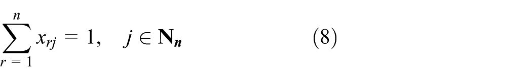
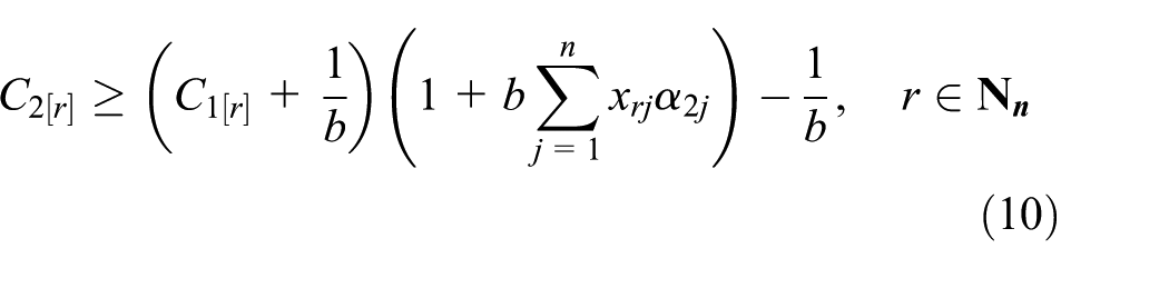
Objective function (6) is to minimize the total completion time of all the jobs. Constraints (7) and (8) ensure that one position in a processing sequence of the jobs can be occupied by only one job, and one job can be scheduled at only one position, respectively. Constraint (9) means that for an optimal processing sequence of jobs, machine M₁ cannot be interrupted. Constraints (10) and (11) establish the relationship between the completion time of job J_j at machines M₁ and M₂. They make sure that the starting time of the jth job to be processed by M₂ is greater than or equal to the completion time of the jth job processed by M₁ and the completion time of (j − 1)th job processed by machine M₂. Constraint (12) confirms the boundary of the decision variables. Constraint (13) confirms that the completion time of each job is greater than zero. Constraint (14) means that the time when M₁ and M₂ can start to work is zero. Thus, every job is available at t₀ = 0. In this way, an MIP model is formulated. However, the computation for solving this problem is exponential with the number of the integer variables in the model. Therefore, it is very difficult to solve the MIP model for the addressed problem when the problem size is large.

Solution method

VNS

Since the time taken to solve the MIP model for F2|p_ij = α_ij(1 +bt), s_ij = δ_ij(1 +bt)|ΣC_2j is exponential with the number of binary variables it is inefficient to apply an exact solution method to obtain an optimal. Therefore, an efficient heuristic approach is preferred to find an optimal or near-optimal solution. VNS algorithm is such a kind of heuristic algorithm. It is a metaheuristic algorithm which can improve the local search by systematically changing the neighborhood structures such that a locally optimal solution can be avoided. The basic scheme of VNS can be found in Mladenovic and Hansen,²⁸ and a good survey is given in the literature.^29–31 It has been proved to be a simple and efficient method for solving combinatorial optimization problems. Thus, this work adopts VNS to solve the scheduling problem of a two-machine flow shop with both the jobs and setup time being deteriorated.

Given a schedule π, let Ψ_k, k ∈ {1, 2, …, K}, denote a neighborhood structure and Ψ_k(π) be a set of schedules obtained using Ψ_k based on π. Therefore, Ψ_k is a scheduling policy for finding better schedules by starting from π. The general VNS can be found in Mladenovic and Hansen²⁸ as presented in Algorithm 1.

Based on the scheme of VNS obtained by Algorithm 1, a detailed VNS algorithm can be developed to solve the scheduling problem F2|p_ij = α_ij(1 +bt), s_ij = δ_ij(1 +bt)|ΣC_2j. To develop a complete VNS algorithm, one needs to determine the construction of the solution, generate an initial solution, and determine the neighborhood structures. In this work, we use the job processing sequence to represent a solution denoted by π = {π₁, …, π_k, …, π_n}, where π_k is the job that is scheduled to be processed in the kth position. Since the VNS is a metaheuristics whose performance is heavily dependent on the initial solution, it is necessary to have a good initial solution. Since the VNS is designed for large-sized problem, we need a computationally efficient method to find a good initial solution. A heuristics is useful. Let Ω₁ and Ω₂ denote the sets of scheduled jobs and unscheduled jobs, respectively. Then, a greedy algorithm (Algorithm 2) is proposed to do so.

Algorithm 1: General VNS algorithm.
Step 1: Initialization:
Step 1.1: Determine the neighborhood structures Ψ_k, k ∈ {1, 2, …, K};
Step 1.2: Give an initial schedule π;
Step 1.3: Set a terminating condition for the algorithm;
Step 2: While the terminating condition is not met do
Step 2.1: Select the first neighborhood structure Ψ₁;
Step 2.2: Whilek ≤ K do
Step 2.2.1: Change the neighborhood structure Ψ_k and generate a solution π, π′ ∈ Ψ_k(π);
Step 2.2.2: If π′ is better than π, then the initial π is replaced by π′ and set k = 1; Otherwise set k = k + 1;
End while
End while

Algorithm 2: Generate an initial schedule π.
Step 1: Set r = 1, Ω₁ = ∅, and Ω₂ = {J₁, J₂, …, J_n};
Step 2: Select a job from Ω₂ and put it into Ω₁;
Step 2.1: Choose job J_j ∈ Ω₂ such that max{(1 + bδ_1j)(1 + bα_1j), (1 + bδ_2j)}(1 + bα_2j) is minimized;
Step 2.2: Put J_j in the rth position, set C_1r = (t₀ + 1/b)(1 + bδ_1j)(1 + bα_1j) − 1/b and C_2r = max{(t₀ + 1/b)(1 + bδ_1j)(1 + bα_1j), (t₀ + 1/b)(1 + bδ_2j)}(1 + bα_2j) − 1/b;
Step 2.3: Update Ω₁ ← Ω₁∪ {J_j} and Ω₂ ← Ω₂\{J_j};
Step 3: Collect the jobs from those with (C_1r + 1/b)(1 + bδ_1j)(1 + bα_1j) − 1/b ≤ C_2r;
Step 3.1: If (C_1r + 1/b)(1 + bδ_1j)(1 + bα_1j) − 1/b ≤ C_2r holds for more than one job, choose the one such that (1 + bδ_1j)(1 + bα_1j) is minimized and put it at the (r + 1)th position;
Step 3.2: If (C_1r + 1/b)(1 + bδ_1j)(1 + bα_1j) − 1/b ≤ C_2r does not hold for any job, then: (1) choose the job such that (1 + bδ_2j)(1 + bα_2j) is minimized and put it at the (r + 1)th position; and (2) C_2r is replaced by C_2(r+1) = max{(C_1r + 1/b)(1 + bδ_1j)(1 + bα_1j), (C_2r + 1/b)(1 + bδ_2j)}(1 + bα_2j) − 1/b, and C_1r is replaced by C_1(r+1) = (C_1r + 1/b)(1 + bδ_1j)(1 + bα_1j) − 1/b;
Step 3.3: Set r ← r + 1;
Step 3.4: Update Ω₁ ← Ω₁∪ {J_j} and Ω₂ ← Ω₂\{J_j};
Step 4: If Ω₂ ≠ Φ, go to Step 3; otherwise go to Step 5;
Step 5: Output an initial schedule π = {π₁, …, π_k, …, π_n}.

The main idea of this algorithm is to make sure that the make-span for completing these jobs to be short since our objective is to minimize the total completion time. By Algorithm 2, an initial schedule is found. Then, we need to design the neighborhood structures to search for an optimal or near-optimal schedule. In Kirlik and Oguz,³⁰ four types of neighborhood structures are given for single-machine scheduling problem with total weighted tardiness minimization as objective, and they are shown to be effective. Thus, based on them, four similar neighborhood structures are developed for the problem addressed here. They are denoted as Ψ₁, Ψ₂, Ψ₃, and Ψ₄ and presented as follows.

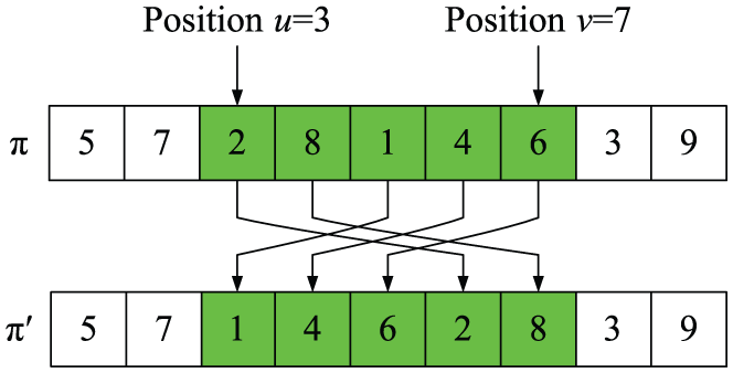
Let u and v denote the uth and vth positions in a schedule and assume that v > u. Then, neighborhood structure Ψ₁ operates as follows: the job at Position u in a schedule is taken away and inserted into Position v. By doing so, the jobs in Position k, k ∈ {u+ 1, …, v}, are shifted one position forward along the initial solution π. This can be illustrated by an example as shown in Figure 4. For this example, the initial schedule is π = [5 7 2 8 1 4 6 3 9] and u = 3 and v = 7. By Ψ₁, Job 2 at Position u = 3 is removed and inserted into Position v = 7, leading to that the jobs at Position k, k ∈ {4, 5, 6, 7}, are shifted one position forward such that a new schedule π′ = [5 7 8 1 4 6 2 3 9] is obtained. We define Insert (π, u, v) as an algorithm for performing Ψ₁ as follows:

Algorithm 3: Insert (π, u, v), or perform Ψ₁.
1. In Schedule π, randomly select a job, assume that its position is u and the job is labeled as π_u;
2. In π, randomly select a position and it is labeled as v such that u ≠ v;
3. Remove π_u from π;
4. Insert π_u to Position v;
5. End.

Figure 4.

An example of insert operation.

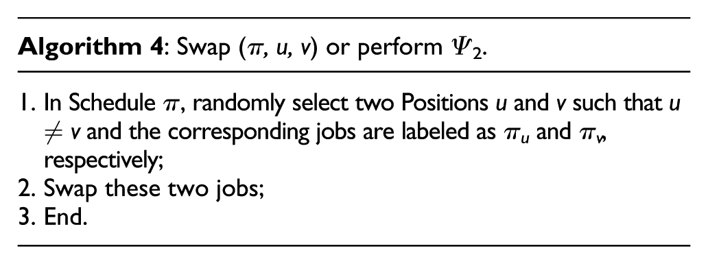
Neighborhood structure Ψ₂ is used to swap two jobs at Positions u and v in π. An example of a swap operation is shown in Figure 5. The initial schedule π = [5 7 2 8 1 4 6 3 9] and u = 3 and v = 7. Then, by swap operation, a new solution π′ = [5 7 6 8 1 4 2 3 9] is obtained. We use an algorithm to define Swap (π, u, v) for Ψ₂ as follows:

Algorithm 4: Swap (π, u, v) or perform Ψ₂.
1. In Schedule π, randomly select two Positions u and v such that u ≠ v and the corresponding jobs are labeled as π_u and π_v, respectively;
2. Swap these two jobs;
3. End.

Figure 5.

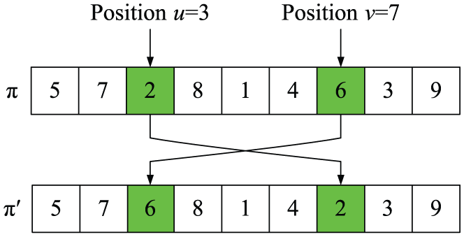
An example of swap operation.

We define two adjacent jobs in a schedule π as a job block. For neighborhood structure Ψ₃, we randomly select two Positions u and v in a schedule π such that u+ 1 < v − 1. These two jobs form a job block denoted as block (π_u, π_u₊₁). Then, the block is inserted into Position (v − 1). Such an operation is 2-optinset operation and is illustrated in Figure 6, where π = [5 7 2 8 1 4 6 3 9], u = 3, and v = 7. The block (π₃, π₄) = (Job 2, Job 8) is then inserted into Position 6, leading to a new solution π′ = [5 7 1 4 6 2 8 3 9]. We use an algorithm to define 2-optinsert (π, u, v) for Ψ₃ as follows:

Algorithm 5: 2-optinsert (π, u, v) or perform Ψ₃.
1. In Schedule π, select a job block (π_u, π_u₊₁) and Position v randomly such that u + 1 < v − 1;
2. Remove the job block (π_u, π_u₊₁) from π;
3. Insert job block (π_u, π_u₊₁) into Position (v − 1) in π;
4. End.

Figure 6.

An example of 2-optinsert operation.

For neighborhood structure Ψ₄, two Positions u and v in a schedule π are selected such that |v − u| ≥ 3 to form two job blocks (π_u, π_u₊₁) and (π_v, π_v₊₁). Then, the positions of job blocks (π_u, π_u₊₁) and (π_v, π_v₊₁) are swapped. Such an operation is called a 2-optswap operation and is illustrated in Figure 7, where π = [5 7 2 8 1 4 6 3 9], u = 3, and v = 6, and job blocks (π₃, π₄) = (Job 2, Job 8) and (π₆, π₇) = (Job 4, Job 6) are formed. Then, they are 2-optswapped to obtain π′ = [5 7 4 6 1 2 8 3 9]. We use an algorithm to define 2-optswap (π, u, v) for Ψ₄ as follows:

Algorithm 6: 2-optswap (π, u, v) or perform Ψ₄.
1. In Schedule π, select two job blocks (π_u, π_u₊₁) and (π_v, π_v₊₁) randomly such that \|v − u\| ≥ 3;
2. Swap job blocks (π_u, π_u₊₁) and (π_v, π_v₊₁);
3. End.

Figure 7.

An example of 2-optswap operation.

Up to now, four neighborhood structures have been proposed. Then, with Algorithm 2 and Ψ₁−Ψ₄, we present the detailed VNS algorithm to find an optimal or near-optimal schedule for problem F2|p_ij = α_ij(1 +bt), s_ij = δ_ij(1 +bt)|ΣC_2j. This algorithm is given as follows:

Algorithm 7: The detailed VNS algorithm to find an optimal or near-optimal schedule for problem F2\|p_ij = α_ij(1 + bt), s_ij = δ_ij(1 + bt)\|ΣC_2j.
Step 1: Create an initial schedule π = {π₁, π₂, …, π_n} using Algorithm 2 and set a value for loop_max as the maximal number of iteration times;
Step 2: Set loop ← 0 and flag ← 0;
Step 3: Whileloop < loop_max do
Step 3.1: Randomly choose two Positions u and v in π such that 1 ≤ u < v ≤ n;
Step 3.2: Ifflag == 0, then perform Insert (π, u, v) to obtain a schedule π′, compute ΣC_2n(π′);
Else ifflag == 1, then perform Swap (π, u, v) to obtain a schedule π′, compute ΣC_2n(π′);
Else ifflag == 2, then perform 2-optinsert (π, u, v) to obtain a schedule π′, compute ΣC_2n(π′);
Else perform 2-optswap (π, u, v) to obtain a schedule π′, compute ΣC_2n(π′);
End if;
Step 3.3: IfΣC_2n(π′) < ΣC_2n(π), then π ← π′ and flag ← 0;
Elseflag ← (flag + 1) mod 4;
End if;
Step 3.4: loop ← loop + 1;
End while
Step 4: Output the optimal or near-optimal solution π* and end.

Lower bounds

It is well known that effective lower bounds can help to evaluate the effectiveness and efficiency of a heuristic algorithm. This work develops two methods to calculate the lower bound. The main idea to obtain the lower bound is to calculate the workloads on the two machines, respectively. Based on this idea, we analyze the lower bounds as follows. Suppose that (Ω₁, Ω₂) is a schedule, where Ω₁ and Ω₂ denote the processing sequence of the jobs. For example, (Ω₁, Ω₂) is a schedule, where Ω₁ = {J₃, J₅, J₆} and Ω₂ = {J₂, J₁, J₄}. Thus, for this schedule, the processing sequence of the jobs is J₃, J₅, J₆, J₂, J₁, J₄. Assume that there are k jobs in Ω₁. Then, we have the following theorem.

Theorem 1

For any job J_i, if $(t_{0} + 1 / b) \times Π_{j = 1}^{i} [(1 + b δ_{1 [j]}) (1 + b α_{1 [j]})] \geq (C_{2 [i - 1]} (Ω_{1}) + 1 / b) \times (1 + b δ_{2 [i]})$ holds, then the first lower bound is $L B_{1} = \sum_{j = 1}^{k} C_{2 [j]} (\underset{1}{Ω}) + (t_{0} + 1 / b) \times (1 + b \times \min_{k + 1 \leq j \leq n} α_{2 [j]}) \times Π_{j = 1}^{k} [(1 + b δ_{1 [j]}) (1 + b α_{1 [j]})] \times \sum_{i = k + 1}^{n} Π_{j = k + 1}^{i} [(1 + b δ_{1 (j)}) (1 + b α_{1 (j)})] - (n - k) / b$ , where (1 +bδ_1(k+1)) × (1 +bα_1(k+1)) ≤ (1 +bδ_1(k+2)) × (1 +bα_1(k+2)) ≤ … ≤ (1 +bδ_1(n)) × (1 +bα_1(n)).

Proof

With the assumption that $(t_{0} + 1 / b) \times Π_{j = 1}^{i} [(1 + b δ_{1 [j]}) (1 + b α_{1 [j]})] \geq (C_{2 [i - 1]} (Ω_{1}) + 1 / b) \times (1 + b δ_{2 [i]})$ , we show the theorem by induction. For the (k+ 1)th job, the completion time is $C_{2 [k + 1]} (Ω_{2}) = (max {t_{0} + 1 / b) \times Π_{j = 1}^{k + 1} [(1 + b δ_{1 [j]}) (1 + b α_{1 [j]})] - 1 / b, (C_{2 [k]} (Ω_{1}) + 1 / b) \times (1 + b δ_{2 [k + 1]}) - 1 / b} + 1 / b) \times (1 + b α_{2 [k + 1]}) - 1 / b \geq (t_{0} + 1 / b) \times Π_{j = 1}^{k + 1} [(1 + b δ_{1 [j]}) (1 + b α_{1 [j]})] \times (1 + b α_{2 [k + 1]}) - 1 / b$ . Similarly, for each job, the total completion time of the ith job is $C_{2 [i]} (Ω_{2}) = (\max {(t_{0} + 1 / b) \times Π_{j = 1}^{i} [(1 + b δ_{1 [j]}) (1 + b α_{1 [j]})] - 1 / b, (C_{2 [i - 1]} (Ω_{1}) + 1 / b) \times (1 + b δ_{2 [i]}) - 1 / b} + 1 / b) \times (1 + b α_{2 [i]}) - 1 / b \geq (t_{0} + 1 / b) \times Π_{j = 1}^{i} [(1 + b δ_{1 [j]}) (1 + b α_{1 [j]})] \times (1 + b α_{2 [i]}) - 1 / b$ , for i = k+ 1, k+ 2, …, n. Thus, the total completion time is $TC (Ω_{1} Ω_{2}) = \sum_{j = 1}^{k} C_{2 [j]} (\underset{1}{Ω}) + \sum_{j = k + 1}^{n} C_{2 [j]} (\underset{2}{Ω}) \geq \sum_{j = 1}^{k} C_{2 [j]} (\underset{1}{Ω}) + (t_{0} + 1 / b) \times Π_{j = 1}^{k} [(1 + b δ_{1 [j]}) (1 + b α_{1 [j]})] \times [\sum_{i = k + 1}^{n} Π_{j = k + 1}^{i} [(1 + b δ_{1 [j]}) (1 + b α_{1 [j]}) (1 + b α_{2 [i]})]] - (n - k) / b \geq \sum_{j = 1}^{k} C_{2 [j]} (\underset{1}{Ω}) + (t_{0} + 1 / b) \times (1 + b \times \min_{k + 1 \leq j \leq n} α_{2 [j]}) \times Π_{j = 1}^{k} [(1 + b δ_{1 [j]}) (1 + b α_{1 [j]})] \times \sum_{i = k + 1}^{n} Π_{j = k + 1}^{i} [(1 + b δ_{1 [j]}) (1 + b α_{1 [j]})] - (n - k) / b$ . Note that $\sum_{j = 1}^{k} C_{2 [j]} (\underset{1}{Ω})$ , $(t_{0} + 1 / b) \times (1 + b \times \min_{k + 1 \leq j \leq n} α_{2 [j]}) \times Π_{j = 1}^{k} [(1 + b δ_{1 [j]}) (1 + b α_{1 [j]})]$ , and (n − k)/b are known and are constant. Thus, a lower bound of TC(Ω₁, Ω₂) can be obtained by minimizing $\sum_{i = k + 1}^{n} Π_{j = k + 1}^{i} [(1 + b δ_{1 [j]}) (1 + b α_{1 [j]})]$ . Mosheiov³² pointed out that the total completion time can be minimized by sequencing the jobs according to the shortest remaining deterioration rate (SRDR) rule. Based on SRDR rule and the assumption that (1 +bδ_1(k+1)) × (1 +bα_1(k+1)) ≤ (1 +bδ_1(k+2)) × (1 +bα_1(k+2)) ≤ … ≤ (1 +bδ_1(n)) × (1 +bα_1(n)), we have that the first lower bound is $\begin{array}{l} L B_{1} = \sum_{j = 1}^{k} C_{2 [j]} (\underset{1}{Ω}) + (t_{0} + 1 / b) \times (1 + b \times \underset{k + 1 \leq j \leq n}{m i n} α_{2 [j]}) \times \prod_{j = 1}^{k} [(1 + b δ_{1 [j]}) (1 + b α_{1 [j]})] \\ \times \sum_{i = k + 1}^{n} \prod_{j = k + 1}^{i} [(1 + b δ_{1 (j)}) (1 + b α_{1 (j)})] - (n - k) / b \end{array}$ . Hence, the theorem holds. ■

In Theorem 1, due to $(t_{0} + 1 / b) \times Π_{j = 1}^{i} [(1 + b δ_{1 [j]}) (1 + b α_{1 [j]})] \geq (C_{2 [i - 1]} (\underset{1}{Ω}) + 1 / b) \times (1 + b δ_{2 [i]})$ , it is known that after machine M₂ completes a job, it always needs to wait for another job that is being processed by M₁. Thus, the make-span depends on the completion time of the jobs on machine M₁.

Theorem 2

For any job J_i, if $(t_{0} + 1 / b) \times Π_{j = 1}^{i} [(1 + b δ_{1 [j]}) (1 + b α_{1 [j]})] \leq (C_{2 [i - 1]} (\underset{1}{Ω}) + 1 / b) \times (1 + b δ_{2 [i]})$ , then the second lower bound is $L B_{2} = \sum_{j = 1}^{k} C_{2 [j]} (\underset{1}{Ω}) + (C_{2 [k]} (Ω_{1}) + 1 / b) \times \sum_{j = k + 1}^{n} Π_{i = k + 1}^{j} [(1 + b δ_{2 (i)}) (1 + b α_{2 (i)})] - (n - k) / b$ , where (1 +bδ_2(k+1)) × (1 +bα_2(k+1)) ≤ (1 +bδ_2(k+2)) × (1 +bα_2(k+2)) ≤ … ≤ (1 +bδ_2(n)) × (1 +bα_2(n)).

Proof

Based on Theorem 1, with the assumption that $(t_{0} + 1 / b) \times Π_{j = 1}^{i} [(1 + b δ_{1 [j]}) (1 + b α_{1 [j]})] \leq (C_{2 [i - 1]} (\underset{1}{Ω}) + 1 / b) \times (1 + b δ_{2 [i]})$ , the completion time of the (k+ 1)th job is $C_{2 [k + 1]} (Ω_{2}) = (\max {(t_{0} + 1 / b) \times Π_{j = 1}^{k + 1} [(1 + b δ_{1 [j]}) (1 + b α_{1 [j]})] - 1 / b, (C_{2 [k]} (Ω_{1}) + 1 / b) \times (1 + b δ_{2 [k + 1]}) - 1 / b} + 1 / b) \times (1 + b α_{2 [k + 1]}) - 1 / b \geq (C_{2 [k]} (Ω_{1}) + 1 / b) \times (1 + b δ_{2 [k + 1]}) \times (1 + b α_{2 [k + 1]}) - 1 / b$ . Similarly, for each job, the total completion time of the ith job is $C_{2 [i]} (Ω_{2}) = (\max {(t_{0} + 1 / b) \times \prod_{j = 1}^{i} [(1 + b \underset{1 [j]}{δ}) (1 + b \underset{1 [j]}{α})] - 1 / b, (C_{2 [i - 1]} (Ω_{1}) + 1 / b) \times (1 + b δ_{2 [i]}) - 1 / b} + 1 / b) \times (1 + b α_{2 [i]}) - 1 / b \geq (C_{2 [k]} (Ω_{1}) + 1 / b) \times \prod_{j = 1}^{i} [(1 + b δ_{1 [j]}) (1 + b α_{1 [j]})] \times (1 + b α_{2 [i]}) - 1 / b$ , for i = k+ 1, k+ 2, …, n. Thus, the total completion time of all the scheduled jobs is $TC (\underset{1}{Ω}, \underset{2}{Ω}) = \sum_{j = 1}^{k} C_{2 [j]} (\underset{1}{Ω}) + \sum_{j = k + 1}^{n} C_{2 [j]} (\underset{2}{Ω}) \geq \sum_{j = 1}^{k} C_{2 [j]} (\underset{1}{Ω}) + (C_{2 [k]} (\underset{1}{Ω}) + 1 / b) \times \sum_{j = k + 1}^{n} Π_{i = k + 1}^{j} [(1 + b δ_{2 (i)}) (1 + b α_{2 (i)})] - (n - k) / b$ . Since $\sum_{j = 1}^{k} C_{2 [j]} (\underset{1}{Ω})$ , C_2[k](Ω₁) + 1/b, and (n − k)/b are constant, the key to obtain the lower bound of TC(Ω₁, Ω₂) is to minimize $\sum_{j = k + 1}^{n} Π_{i = k + 1}^{j} [(1 + b δ_{2 (i)}) (1 + b α_{2 (i)})]$ . Based on SRDR rule and the assumption that (1 +bδ_2(k+1)) × (1 +bα_2(k+1)) ≤ (1 +bδ_2(k+2)) × (1 +bα_2(k+2)) ≤ … ≤ (1 +bδ_2(n)) × (1 +bα_2(n)), we have that the second lower bound is $L B_{2} = \sum_{j = 1}^{k} C_{2 [j]} (\underset{1}{Ω}) + (C_{2 [k]} (Ω_{1}) + 1 / b) \sum_{j = k + 1}^{n} Π_{i = k + 1}^{j} [(1 + b δ_{2 (i)}) (1 + b α_{2 (i)})] - (n - k) (1 / b)$ . Hence, the theorem holds. ■

In Theorem 2, due to $(t_{0} + 1 / b) \times Π_{j = 1}^{i} [(1 + b δ_{1 [j]}) (1 + b α_{1 [j]})] \leq (C_{2 [i - 1]} (Ω_{1}) + 1 / b) \times (1 + b δ_{2 [i]})$ , it is known that after a job is processed on machine M₁, it always need to wait for machine M₂ to be released. Thus, the make-span depends on the completion time of the jobs on Machine M₂. For the addressed scheduling problem (F2|p_ij = α_ij(1 +bt), s_ij = δ_ij(1 +bt)|ΣC_2j) in this work, LB₁ and LB₂ can be obtained when M₁ or M₂ is bottleneck for all the time. However, for some cases, during sometime, M₁ is the bottleneck, while M₂ is the bottleneck during other time. It is easy to obtain that for these cases, the lower bound of the completion time of the jobs is

LB = \max {L B_{1}, L B_{2}}

(15)

Numerical results

To evaluate the performance of Algorithms 2 and 7, computational experiments are carried out. Algorithms 2 and 7 are coded in C and run on a Pentium III 2.20-GHz personal computer (PC) with 2.00-GB RAM. The MIP was coded in software LINGO 11 solver on the same computer. The considered scheduling problem (F2|p_ij = α_ij(1 +bt), s_ij = δ_ij(1 +bt)|ΣC_2j) can be solved optimally by the MIP when the number of jobs is <20, but for a medium- or large-sized problems, an exactly optimal schedule cannot be found within a reasonable computational time using the MIP. As a metaheuristic algorithm, the proposed VNS may not achieve a global optimum. Therefore, three sets of experiments are conducted in this article. For the first experiment, we compare the VNS with MIP for the considered scheduling problem with different sizes (n = 10, 20) to evaluate the effectiveness and efficiency of the VNS. For the second experiment, we compare the VNS with lower bound when the problem size is medium or large. For the third experiment, we evaluate the improvement made by the VNS with respect to the initial schedule obtained by the greedy algorithm.

Parameter setting

All the data were randomly generated from the discrete uniform distributions but with different parameters. In the second experiment, nine different sizes of the jobs n = (10, 15, 20, 25, 30, 35, 40, 45, 50) are used to test the proposed method, while five different sizes of the jobs n = (10, 20, 30, 40, 50) are used to do so in the third experiment. For each size of the jobs, the normal processing time for M₁ and M₂ is generated from the discrete uniform distributions [1, 10], and the normal setup time for M₁ and M₂ is generated from the discrete uniform distributions [1, 4]. For all the tests, t₀ = 0 is set, and the deterioration index are set to be three different values, that is, b = 0.1, 2, and 5 for small, medium, and large, respectively. We repeat 10 times for each approach to obtain the average values for all the tests.

It is vitally important to set the parameters since the performance of the VNS is usually sensitive to them. In this article, for the proposed VNS, we have only one parameter: loop_max. In order to determinate loop_max for the VNS, we examine the problem with its size being 20 (n = 20) since we can analyze the effect of loop_max by comparing with the optimal solution obtained via the MIP. The performance of the VNS can be measured by the percentage of the relative percentage deviation (RPD) from the obtained solution to the optimal solution. 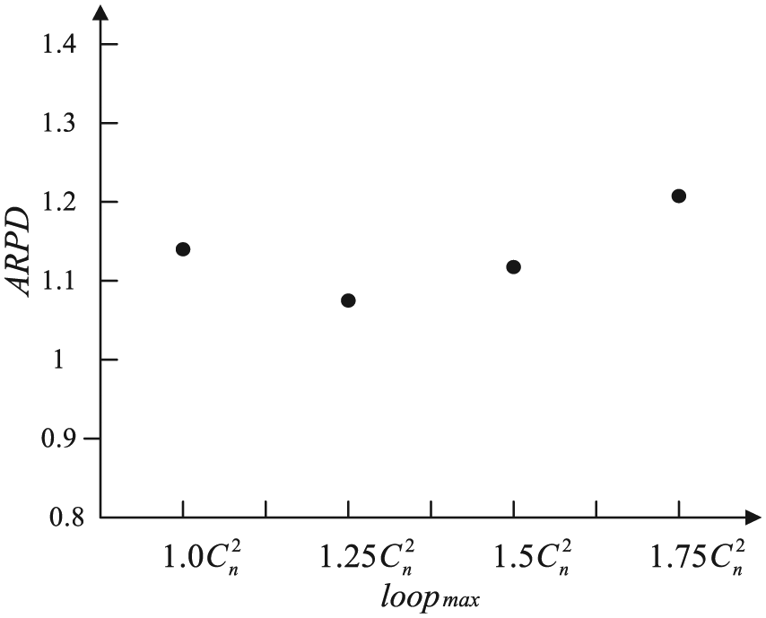The RPD is given as $RPD = (\sum C_{2 [j]} - \sum C_{2 [j]}^{*}) / \sum C_{2 [j]}^{*} \times 100 %$ , where $\sum C_{2 [j]}$ is the objective value obtained by the VNS and $\sum C_{2 [j]}^{*}$ is the optimal solution found by the MIP. Due to the properties of the addressed scheduling problem, the considered levels are as follows: ${1.0 C}_{n}^{2}$ , ${1.25 C}_{n}^{2}$ , ${1.5 C}_{n}^{2}$ , and ${1.75 C}_{n}^{2}$ , where n is the number of jobs. Thus, we used a single-factor analysis of variance (ANOVA) approach to analyze the solution. Figure 8 shows the average RPD (ARPD) at different considered levels of parameter loop_max. From Figure 8, it can be seen that the loop_max of ${1.25 C}_{n}^{2}$ performs better than the others. Thus, the loop_max of ${1.25 C}_{n}^{2}$ is chosen for the proposed VNS in the experiments.

Figure 8.

The ARPD at different considered levels of parameter loop_max.

Experiment 1

In this experiment, we select two different sizes of jobs n = (10, 20) to compare the VNS with MIP, since they can be solved by LINGO 11 within reasonable computational time (3600 s). For each experiment, the VNS repeats 10 times to obtain the maximum and minimum values of the objective function. The deviations are used to show the performance comparison between VNS and MIP, and it is formulated as Dev. = (The minimum value of the objective obtained by VNS) − (The value of the objective obtained by MIP).

The computational time of the MIP and the deviations are shown in Table 1. It can be observed that for all the cases, Dev. is zero, when the job size is 10 and 20. This experiment shows that the VNS can find the optimal solution when the job size is small (n ≤ 20). Most of the maximum values are greater than the minimum values except that they are equal for one case as shown by bold values since the scheduling problem with deteriorations jobs is a combinatorial optimization problem and has a strong relationship with the starting processing time for every job. When the size is 10 and 20, almost all the tests can be solved by the MIP within reasonable computational time (287 s), except that for two tests, it takes 3637 and 1828 s as shown with bold values in Table 1, respectively. The shortest time is 2 s only. The average time taken for solving these problems with job sizes 10 and 20 is 30.65 and 54.7 s, without considering the two worst cases with the computational time 3637 and 1828 s, respectively. As the size increases, it would be more complex and difficult for the MIP to solve.

Table 1.

Comparative results for the solution of VNS and MIP with n = 10 and n = 20.

No. of jobs, n = 10						No. of jobs, n = 20
No.	VNS		MIP		Dev.	No.	VNS		MIP		Dev.
No.	Maximum	Minimum	Solution	Time	Dev.	No.	Maximum	Minimum	Solution	Time	Dev.
1	0.673e+03	0.662e+03	0.662e+03	11	0	1	3.646e+05	3.635e+05	3.635e+05	37	0
2	0.544e+03	0.531e+03	0.531e+03	49	0	2	3.359e+05	3.353e+05	3.353e+05	12	0
3	1.128e+03	1.114e+03	1.114e+03	21	0	3	1.266e+05	1.261e+05	1.261e+05	17	0
4	1.004e+03	1.004e+03	1.004e+03	68	0	4	3.980e+05	3.966e+05	3.966e+05	62	0
5	0.983e+03	0.964e+03	0.964e+03	47	0	5	7.893e+05	7.882e+05	7.882e+05	26	0
6	0.866e+03	0.847e+03	0.847e+03	13	0	6	6.838e+05	6.823e+05	6.823e+05	3637	0
7	0.553e+03	0.537e+03	0.537e+03	47	0	7	4.849e+05	4.846e+05	4.846e+05	43	0
8	2.211e+03	2.119e+03	2.119e+03	36	0	8	2.266e+05	2.256e+05	2.256e+05	103	0
9	0.988e+03	0.947e+03	0.947e+03	24	0	9	3.203e+05	3.191e+05	3.191e+05	55	0
10	1.639e+03	1.616e+03	1.616e+03	20	0	10	5.037e+05	5.012e+05	5.012e+05	16	0
11	3.253e+03	3.244e+03	3.244e+03	9	0	11	3.088e+05	3.064e+05	3.064e+05	11	0
12	1.103e+03	1.083e+03	1.083e+03	16	0	12	3.661e+05	3.630e+05	3.630e+05	1828	0
13	1.284e+03	1.270e+03	1.270e+03	2	0	13	3.854e+05	3.828e+05	3.828e+05	19	0
14	1.344e+03	1.333e+03	1.333e+03	49	0	14	1.834e+05	1.804e+05	1.804e+05	29	0
15	1.646e+03	1.624e+03	1.624e+03	51	0	15	8.066e+05	8.060e+05	8.060e+05	16	0
16	1.102e+03	1.072e+03	1.072e+03	2	0	16	1.343e+05	1.332e+05	1.332e+05	58	0
17	0.821e+03	0.781e+03	0.781e+03	18	0	17	7.332e+05	7.323e+05	7.323e+05	81	0
18	0.802e+03	0.774e+03	0.774e+03	81	0	18	6.352e+05	6.339e+05	6.339e+05	287	0
19	0.585e+03	0.538e+03	0.538e+03	44	0	19	5.884e+05	5.880e+05	5.880e+05	100	0
20	1.285e+03	1.266e+03	1.266e+03	5	0	20	4.190e+05	4.186e+05	4.186e+05	12	0
Average				30.65		Average				54.7

MIP: mixed integer programming; VNS: variable neighborhood search.

Experiment 2

To investigate the effectiveness of the proposed VNS for such problems, it is compared with the lower bound. In this experiment, the test problem size is n = 10, 15, 20, 25, 30, 35, 40, 45, and 50, respectively. For each test, it repeats 10 times to obtain the mean solution, and the mean absolute percentage of deviation is defined as follows: $% D = ((The optimal solution of VNS - LB) / LB) \times 100 %$ .

Table 2 shows the performance of the proposed VNS, where the values of %D are presented. It can be observed that the average deviation percentages are zero for the small-sized problem (n ≤ 20). Also, the VNS can achieve the optimal solution for small-sized problems, which is consistent with the results obtained in Experiment 1. The average deviation percentages are <3% for almost all the test problems. We note that the average deviation percentage becomes larger when the deterioration rate index is larger. This is because the large deterioration rate index can make the actual processing time and setup time become much longer. The experiment shows that the VNS can be used to solve the addressed scheduling problem effectively, especially when the problem size is large. In summary, it follows from Table 2 that a near-optimal or optimal schedule can be found by the proposed VNS even though deterioration rate index is relevantly large. In other words, the proposed VNS method is applicable and effective to the addressed problem.

Table 2.

Comparative results for the solution of VNS with lower bound.

Job size (n)	b = 0.1	b = 2	b = 5	Average %D
10	0.000	0.000	0.000	0.00
15	0.000	0.000	0.000	0.00
20	0.000	0.000	0.000	0.000
25	0.162	0.174	0.193	0.176
30	0.155	0.189	0.192	0.179
35	0.221	0.295	0.293	0.270
40	0.533	0.512	0.593	0.546
45	1.183	1.219	1.363	1.255
50	2.152	2.382	2.860	2.465
Average	0.490	0.530	0.610	0.543

Experiment 3

To investigate the performance of the proposed VNS, it is compared with greedy algorithm in order to evaluate the improvements made by the VNS. In this experiment, the test problem size is n = 10, 20, 30, 40, and 50, respectively. For each test, the VNS runs 10 times to obtain an average solution value. We define the percentage improvement (PI_VG) as $P I_{V G} = ((The optimal solution of greedy algorithm - VNS) / VNS) \times 100 %$ , where VNS is the optimal or near-optimal solution obtained by the VNS.

It follows from Experiment 1 that the optimal solution can be found by MIP within reasonable computational time. However, when the problem size is >20 (n > 20), it may not be able to find an optimal solution by the MIP within a reasonable computational time (3600 s). For such cases, VNS algorithm is used to obtain an optimal or near-optimal solution. As shown in Table 3, such a solution can be obtained within 3 s even if the number of jobs is 50. Therefore, the VNS algorithm is computationally efficient.

Table 3.

Improvements by performing VNS (in seconds).

Job size (n)	b	VNS time (s)	Greedy algorithm time (s)	%PI_VG
10	0.1	1.00	1.00	2.23
	2	1.00	1.00	2.64
	5	1.00	1.00	2.74
20	0.1	1.00	1.00	2.44
	2	1.00	1.00	2.54
	5	1.00	1.00	2.58
30	0.1	2.00	2.00	2.33
	2	2.00	2.00	2.51
	5	2.00	2.00	2.52
40	0.1	3.00	2.00	2.44
	2	3.00	2.00	2.60
	5	3.00	2.00	2.44
50	0.1	3.00	2.00	2.47
	2	3.00	2.00	2.63
	5	3.00	2.00	2.65
Average		2.00	1.60	2.517

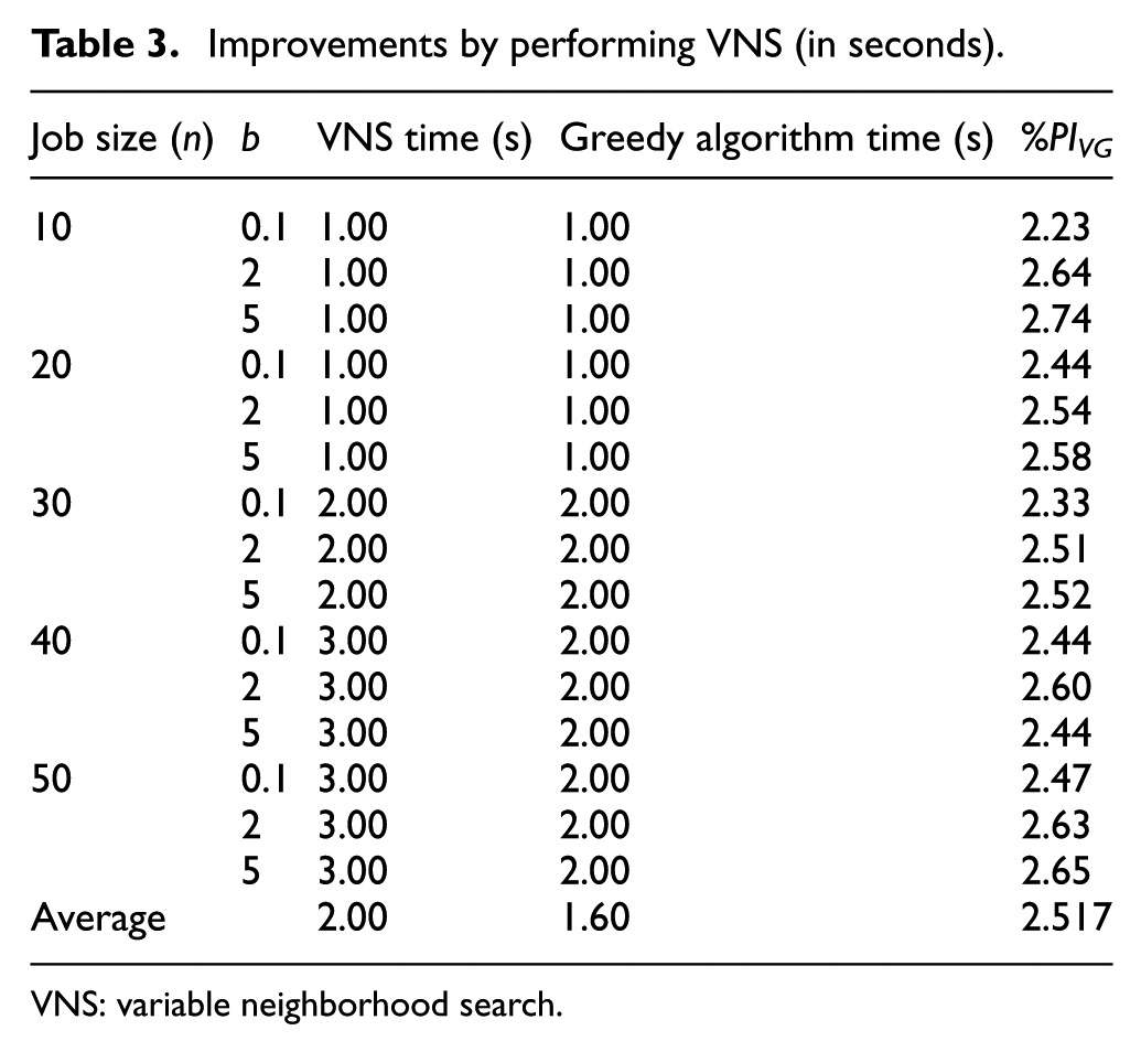
VNS: variable neighborhood search.

It can be seen from Table 3 that the values of PI_VG are increasing as the deterioration rate index of jobs increases for different job sizes except n = 40. Also, we note that for all the tests, the VNS makes a significant improvement with respect to the initial schedule found by the greedy algorithm, especially when b is large. This can be explained as that the small value of b leads to a shorter make-span for this considered problem, and it implies that the greedy algorithm may obtain a better solution when the value of b is small. All in all, the VNS can be used to solve the addressed scheduling problem effectively and efficiently, and it can also make further improvement to obtain a near-optimal or optimal solution compared with the greedy algorithm. Note that the proposed VNS is a metaheuristics other than a simple dispatching rule. Thus, from Table 3, we can conclude that the proposed VNS outperforms a simple heuristic method.

Conclusion

In some production processes, jobs may be subject to deterioration that should be taken into account in scheduling such systems. The scheduling problem of a two-machine flow shop with time-dependent deteriorating jobs and setup time is studied in this article. Although significant studies on scheduling problem of scheduling a two-machine flow shop with time-dependent deteriorating jobs have been done, the existing studies assume that job setup time and its deterioration can be neglected or integrated into the processing time. However, by doing so, the performance of the obtained schedule is not good enough. As far as the authors know, there is no research report on scheduling a two-machine flow shop with both time-dependent deteriorating jobs and setup time. To solve such a challenging problem, the problem is formulated as a MIP model. For small-sized problem, with this model, an optimal schedule can be found using a commercial software tool. For medium- and large-sized problem, a VNS is proposed to find an optimal or near-optimal solution. Since the performance of a VNS is sensitive to the initial solution, a greedy algorithm is developed to find good initial solution for the VNS to improve the performance of the proposed method. Also, lower bounds are presented for performance evaluation. Numerical experiments with different sizes are used to test performance of the proposed method. Results show that using the proposed VNS, an optimal or near-optimal solution can be obtained. Also, the proposed VNS is computationally efficient and outperforms a simple heuristic method. Thus, the proposed VNS is applicable to practical problems.

The existing studies show that performance can be improved using group technology. It is our future work to study how group technology can be used to solve the scheduling problem addressed in this article.

Footnotes

Academic Editor: ZhiWu Li

Declaration of conflicting interests

The author(s) declared no potential conflicts of interest with respect to the research, authorship, and/or publication of this article.

Funding

The author(s) disclosed receipt of the following financial support for the research, authorship, and/or publication of this article: This work was supported in part by Science and Technology Development Fund (FDCT) of Macau under Grants 065/2013/A2 and 102/2013/A, National Natural Science Foundation of China under Grant 61273036.

References

Laalaoui

Bouguila

Pre-run-time scheduling in real-time systems: current researches and artificial intelligence perspectives. Expert Syst Appl 2014; 41: 2196–2210.

Zhang

Qian

. Agent and cyber-physical system based self-organizing and self-adaptive intelligent shopfloor. IEEE T Ind Inform. Epub ahead of print 20 October 2016. DOI: 10.1109/TII.2016.2618892.

Zhang

Ren

Liu

. A big data analytics architecture for cleaner manufacturing and maintenance processes of complex products. J Clean Prod 2017; 142: 626–641.

Zhang

Wang

Liu

. Game theory based real time shop floor scheduling strategy and method for cloud manufacturing. Int J Intell Syst 2017; 32: 437–463.

Bai

. Optimal one-wafer cyclic scheduling and buffer space configuration for single-arm multicluster tools with linear topology. IEEE T Syst Man Cy: A 2016; 46: 1456–1467.

Zhou

MC.

Modeling, analysis and control of dual-arm cluster tools with residency time constraint and activity time variation based on Petri nets. IEEE T Autom Sci Eng 2012; 9: 446–454.

Zhou

MC.

Schedulability analysis and optimal scheduling of dual-arm cluster tools with residency time constraint and activity time variation. IEEE T Autom Sci Eng 2012; 9: 203–209.

Chu

. Petri net modeling and cycle time analysis of dual-arm cluster tools with wafer revisiting. IEEE T Syst Man Cy: A 2013; 43: 196–207.

Zhou

Bai

. Short-term scheduling of crude oil operations in refinery with high fusion point oil and two transportation pipelines. Enterp Inform Syst 2016; 10: 581–610.

10.

Gordon

Potts

Strusevich

. Single machine scheduling models with deterioration and learning: handling precedence constraints via priority generation. J Sched 2008; 11: 357.

11.

Cheng

Bachman

. Three scheduling problems with deteriorating jobs to minimize the total completion time. Inform Process Lett 2002; 81: 327–333.

12.

Zhu

Sun

Chu

. Due-window assignment and scheduling with multiple rate-modifying activities under the effects of deterioration and learning. Math Probl Eng 2011; 2011: 151563 (19 pp.).

13.

Gupta

JND

Gupta

. Single facility scheduling with nonlinear processing times. Comput Ind Eng 1988; 14: 387–393.

14.

Gawiejnowicz

Time-dependent scheduling. Berlin: Springer, 2008.

15.

Lee

WC.

Single-machine group-scheduling problems with deteriorating setup times and job-processing times. Int J Prod Econ 2008; 115: 128–133.

16.

Wang

Lin

Shan

Single-machine group scheduling problems with deteriorating jobs. Int J Adv Manuf Tech 2008; 39: 808–812.

17.

Wang

Gao

Wang

. Single machine group scheduling with general linear deterioration to minimize the make-span. Int J Adv Manuf Tech 2009; 43: 146–150.

18.

Zhang

Yan

GL.

Single-machine group scheduling problems with deteriorated and learning effect. Appl Math Comput 2010; 216: 1259–1266.

19.

Bai

Huang

Single-machine group scheduling with general deterioration and learning effects. Appl Math Model 2012; 36: 1267–1274.

20.

Lee

WC.

Two-machine flow-shop scheduling to minimize mean flow time under linear deterioration. Int J Prod Econ 2006; 103: 572–584.

21.

Wang

Cheng

TCE

. A branch-and-bound algorithm for solving a two-machine flow shop problem with deteriorating jobs. Comput Oper Res 2010; 37: 83–90.

22.

Wang

CTD

Cheng

TCE

. Minimizing total completion time in a two-machine flow-shop with deteriorating jobs. Appl Math Comput 2006; 180: 185–193.

23.

Shiau

Lee

. Two-machine flow-shop scheduling to minimize mean flow-time under simple linear deterioration. Int J Adv Manuf Tech 2007; 34: 774–782.

24.

Yang

Wang

JB.

Minimizing total weighted completion time in a two-machine flow shop scheduling under simple linear deterioration. Appl Math Comput 2011; 217: 4819–4826.

25.

Cheng

Tadikamalla

Shang

. Bicriteria hierarchical optimization of two-machine flow shop scheduling problem with time-dependent deteriorating jobs. Eur J Oper Res 2014; 234: 650–657.

26.

Allahverdi

Cheng

TCE

. A survey of scheduling problems with setup times or costs. Eur J Oper Res 2008; 187: 985–1032.

27.

Allahverdi

Gupta

JND

Aldowaisan

A review of scheduling research involving setup considerations. Omega: Int J Manage S 1999; 27: 219–239.

28.

Mladenovic

Hansen

Variable neighborhood search. Comput Oper Res 1997; 24: 1097–1100.

29.

Hansen

Mladenovic

Perez

JAM

. Variable neighborhood search: methods and applications. Ann Oper Res 2010; 175: 367–407.

30.

Kirlik

Oguz

A variable neighborhood search for minimizing total weighted tardiness with sequence dependent setup times on a single machine. Comput Oper Res 2012; 39: 1506–1520.

31.

Xiong

Xing

Wang

. Minimizing the total completion time in a distributed two stage assembly system with setup times. Comput Oper Res 2014; 47: 92–105.

32.

Mosheiov

Scheduling jobs under simple linear deterioration. Comput Oper Res 1994; 21: 653–659.

33.

Lee

ZS.

Group scheduling with deteriorating jobs to minimize the total weighted number of late jobs. Appl Math Comput 2012; 218: 8750–8757.

34.

Lee

Chung

YH.

Scheduling deteriorating jobs on a single machine with release times. Comput Ind Eng 2008; 54: 441–452.

35.

Wang

Sun

LY.

Single-machine group scheduling with decreasing linear deterioration setup times and job processing times. Int J Adv Manuf Tech 2010; 49: 765–772.

Total completion time minimization for scheduling of two-machine flow shop with deterioration jobs and setup time

Abstract

Keywords

Introduction

Problem description and formulation

Problem description

Problem formulation

Solution method

VNS

Lower bounds

Theorem 1

Proof

Theorem 2

Proof

Numerical results

Parameter setting

Experiment 1

Experiment 2

Experiment 3

Conclusion

Footnotes

Declaration of conflicting interests

Funding

References